Article

Illumination Tolerance for Visual Navigation with the Holistic Min-Warping Method

1
Computer Engineering, Faculty of Technology, Bielefeld University, Bielefeld D-33594, Germany
2
Center of Excellence "Cognitive Interaction Technology", Bielefeld University, Bielefeld D-33594, Germany
*
Author to whom correspondence should be addressed.
Robotics 2014, 3(1), 22-67; https://doi.org/10.3390/robotics3010022
Submission received: 15 December 2013 / Revised: 24 January 2014 / Accepted: 27 January 2014 / Published: 13 February 2014
(This article belongs to the Special Issue Robot Vision)

Abstract

:
Holistic visual navigation methods are an emerging alternative to the ubiquitous feature-based methods. Holistic methods match entire images pixel-wise instead of extracting and comparing local feature descriptors. In this paper we investigate which pixel-wise distance measures are most suitable for the holistic min-warping method with respect to illumination invariance. Two novel approaches are presented: tunable distance measures—weighted combinations of illumination-invariant and illumination-sensitive terms—and two novel forms of “sequential” correlation which are only invariant against intensity shifts but not against multiplicative changes. Navigation experiments on indoor image databases collected at the same locations but under different conditions of illumination demonstrate that tunable distance measures perform optimally by mixing their two portions instead of using the illumination-invariant term alone. Sequential correlation performs best among all tested methods, and as well but much faster in an approximated form. Mixing with an additional illumination-sensitive term is not necessary for sequential correlation. We show that min-warping with approximated sequential correlation can successfully be applied to visual navigation of cleaning robots.

1. Introduction

We first compare feature-based to holistic methods (Section 1.1), recapitulate the holistic min-warping method (Section 1.2), discuss the approaches to illumination invariance taken by feature-based and holistic methods (Section 1.3), and outline the contributions and the structure of the paper (Section 1.4).

1.1. Feature-Based vs. Holistic Methods

In many application domains—e.g., stereo matching, motion detection, pose estimation, construction of 3D models, pattern matching, image registration, or image retrieval—computer and robot vision is presently dominated by “feature-based” approaches. Feature-based methods (i) detect key-points like corners and only extract feature descriptors from their vicinity; (ii) perform complex transformations into feature descriptors and match feature descriptors between images; and (iii) typically require high-resolution images [1,2,3,4,5]. A number of feature detectors and descriptors have been developed, examples being the wide-spread FAST detector [6] and the SIFT [7] and SURF detectors and descriptors [8], and the modern binary descriptors such as BRIEF [9,10], ORB [11], or FREAK [12]. In robot navigation, matches between features are either used for estimating ego-motion between camera postures from two images (such as in visual odometry, see [13,14]), for estimating the metrical position of the corresponding landmark in a geometrical map [15,16,17,18], or for place recognition [19]. Together with subsequent outlier processing (like RANSAC) and n-point methods [14], feature-based methods can reliably estimate the relative posture between two images in 5 dimensions (up to scale).
For visual robot navigation, an emerging alternative to feature-based methods are “holistic” methods which (i) use the entire image (without feature extraction); (ii) compare images as they are (with only moderate preprocessing) by pixel-wise distance measures; and (iii) work on low-resolution images (typically on panoramic images). Most holistic methods have their origin in models of insect visual navigation; also the holistic min-warping method [20] used as an example in this paper has a biologically plausible counter-part [21]. Social insects such as bees, ants, and wasps return to important places (nest locations, food sites) by using visual information (reviews: [22,23]). Their tiny brains with mostly local interconnections and the low visual resolution of their compound eyes make it unlikely that insects employ feature-based methods for navigation. There is a general agreement among modelers that insects probably use holistic methods [21,24,25,26,27,28,29,30].
We presented a classification of holistic local visual homing methods in [20] which we recapitulate here in modified form for the reader’s convenience. Local visual homing methods take a panoramic current view and a snapshot captured at the goal location and compute an azimuthal rotation estimate between the two images and a home vector pointing from the current to the snapshot location. At the present stage of development, all methods assume a movement of the agent in the plane. There are presently five classes of holistic methods: parameter methods, DID methods, visual compass methods (which are part of local visual homing methods), warping methods, and multi-snapshot methods:
  • In parameter methods, entire images are reduced to parameter vectors, and homing to a goal location is achieved by a gradient descent in a distance function between parameter vectors. An extremely parsimonious example is the Average Landmark Vector (ALV) model where the parameter vector comprises just two coordinates and a compass angle [31,32]. This model explains some observations in experiments with bees [33], crickets [34], and desert ants [27]. Our experience shows that parameter methods do not achieve the same navigation quality in robot experiments as other holistic methods. However, these methods may be useful for loop-closure detection [35,36].
  • DID methods (descent in image distances) are based on the observation that, if compass-aligned images are used, the image distance (e.g., pixel-wise Euclidean distance) between two panoramic images increases smoothly with increasing spatial distance between their capture points [25,26,37,38]. Therefore, a gradient descent in the spatial image distance function between current images and snapshot image will lead the agent back to the snapshot location (robot experiments: [39]). Since the gradient has to be estimated by sampling the image distance function at three non-collinear points, test steps need to be inserted into the homing process [25]. This can be avoided by capturing just a single image and predicting two images as if two short test steps (in perpendicular directions) had been executed from the capture position of the real current image [40,41,42].
  • Several visual compass methods have been developed—most of them in the DID framework—which extract the azimuthal orientation difference from two panoramic images [25,26,35,36,37,38,43,44,45,46,47]. Two panoramic images are rotated relative to each other in azimuthal direction and a pixel-wise distance is computed. The minimum location in this rotational image distance function approximately corresponds to the difference in azimuthal orientation between the two images and can be used to align the two images as if they had been captured in the same azimuthal (compass) direction. These methods can be used for aligning images prior to a descent in image distances (see above), for loop-closure detection [35,36], and for multi-snapshot methods (see below).
  • Warping methods [20,21,48,49,50,51] distort one of the images according to a simulated movement and compare the distorted image and the second image by some pixel-wise distance measure. A search for the minimal distance through all movement parameters yields both the estimated home vector and the estimated orientation difference between the two images. Warping has been applied to navigation in topological maps [50,52,53]. The min-warping method [20] addressed in this paper has successfully been applied to cleaning robot control [54,55].
  • Multi-snapshot methods [28,56] form a novel class which takes a middle ground between visual compass and warping methods. Instead of characterizing a goal location by a single panoramic snapshot image, multiple snapshots are collected in the vicinity of the goal location. Each snapshot is captured while the agent faces the goal location. A rotational image distance function (visual compass) is computed between a current view and all snapshots. The best minimum among all snapshots it taken to orient the agent towards the goal. It is our impression that these methods are currently the most convincing model of insect navigation, but it still has to be explored how they perform under changes in illumination.
We feel that, despite the dominance and success of feature-based methods in navigation, holistic methods deserve attention for several reasons:
(1)
Even at the present, relatively early stage in their development, holistic method are almost competitive with feature-based methods with respect to their computational effort. Two properties of holistic methods have a conflicting influence: Low visual resolution promises short computation times whereas the fact that the entire image is used increases the computational effort. The min-warping method—which is among the most complex holistic methods due to its systematic parameter search—requires about 16 ms to compute a home vector and compass estimate from two low-resolution panoramic images ( 288 × 30 pixels) on a modern CPU (Intel i7, 2.3 GHz); for a partial search around a coarse estimate ( 1 / 4 of the search range for each parameter), less then 6 ms are required (96 steps in both parameters, single search). Calonder et al. [10] report times between 3 ms and 7 ms for different versions of their BRIEF descriptor (detection, descriptor computation, and matching of 512 key points, but without RANSAC and n-point method; 2.66 GHz Intel x86-64 CPU).
(2)
Holistic methods exhibit a very regular algorithmic structure—e.g., distances between all pairs of image columns are computed in the first phase of min-warping—and are therefore perfectly suited for an efficient implementation on SIMD units of modern CPUs (SSE, AVX; NEON). For these two reasons, holistic methods may be particularly suitable for consumer market robots (e.g., cleaning or lawn-mowing robots) and for flying robots which typically have limited onboard processing power due to constraints in cost, weight, and battery power.
(3)
Despite their simplicity, some holistic navigation models have been successfully applied to real-world images from outdoor environments [25,26,56] and for indoor navigation of cleaning robots [54,55]. At least for rotation estimation it has been observed that holistic methods perform better than feature-based approaches [57] which seem to be susceptible to calibration errors. Milford [58] demonstrated that place recognition is possible with extremely low visual resolution if the temporal sequence of images is considered. For these reasons we are optimistic that holistic methods can be competitive with feature-based methods with respect to their navigation performance. However, an extensive comparison of feature-based vs. holistic methods is still missing.
(4)
Holistic methods use all available information from an image pair and may therefore be superior to feature-based methods in environments with few suitable features (e.g., corners), such as natural outdoor environments; however, this assumption needs experimental verification.
(5)
We know that min-warping works well in very different visual environments, e.g., in computer simulations with random wall textures without easily discernible landmark features and in different, unmodified real rooms (labs, apartments) [55].
In a recent paper on visual place recognition, Milford [58] discusses advantages and drawbacks of feature-based methods and of alternative methods using low-resolution images (which we would call “holistic”). According to Milford, feature-based approaches “exhibit desirable properties such as scale and rotation invariance, and a limited degree of illumination invariance”. However, “feature-based approaches require a feature detector that is suitable for the type of environment”, thus requiring a selection or training phase. He points out that “feature-based techniques may also fail since visual features can change radically over day-night, weather and seasonal cycles”. These techniques “generally require relatively high-resolution, crisp and noise-free imagery”. In contrast, pixel-by-pixel comparison techniques (as they are also presented in this paper) only need low-resolution images and have the advantage of “not requiring assumptions about the type of visual features in the environment”. However, additional stages are required where the images are transformed (e.g., shifted by a range of offsets) before the pixel-wise distance measures can be applied—in min-warping, this is achieved by computing matches between all pairs of image columns in the two images in multiple versions with different vertical scaling; the systematic search in the second phase selects a subset of these column distances.
Having to apply image transformations before a pixel-wise matching is possible explains a limitation of existing holistic methods: The number of parameters of this transformation has to be kept small, e.g., by limiting movement of the agent to the plane (two parameters since estimation is only possible up to scale). This is also the case in min-warping which assumes a panoramic camera with vertical optical axis with respect to the plane and a flat environment without additional degrees of freedom (changes in height, tilt of the robot) and is thus currently limited to wheeled robots and non-natural environments. In contrast, featured-based methods in combination with n-point methods can estimate relative movement in five degrees of freedom (up to scale).
Holistic methods have received far less attention by the computer-vision community than feature-based methods. We feel that it may still be too early in their development to venture a performance competition with sophisticated feature-based methods—judging from an earlier study where SIFT was applied to local visual homing [59], we actually consider it likely that, at least on the indoor image databases used in this paper, feature-based methods would perform as well as or better than min-warping. However, we think that the insights on illumination tolerance for different distance measures gained in this paper are an important step to make holistic methods more competitive, at least for the min-warping method investigated here. Moreover, for feature-based methods, a number of studies have been dedicated to the comparative evaluation of different feature detectors and descriptors for different applications [1,2,5,17,18,19] indicating that there may be no single method suitable for all applications. A systematic study exploring the application of feature-based methods for local visual homing with panoramic images is not yet available, and would also be beyond the scope of this paper.

1.2. Min-Warping, a Holistic Local Visual Homing Method

The holistc “min-warping” method [20] studied in this paper interrelates two panoramic, monochrome images under the assumption that they have been captured by a panoramic camera with an optical axis vertical to the movement plane and that the robot carrying the camera moves in a flat environment. Min-warping is a local visual homing method: From the two panoramic images captured at different points, it computes two angles, a bearing angle describing the direction from one capture point to the other (alternatively expressed as a unit-length “home vector”), and a rotation angle expressing the azimuthal rotation between the two images (also called “visual compass”). Home vector and visual compass can either be used to approach a target location where the snapshot was taken (by following the home vectors in Section 5), or they can be used to obtain a position estimate by triangulating multiple snapshots with known positions (see Section 7). The latter application of min-warping is the basis of the visual lane-control method for domestic cleaning robots presented in [54,55]. Here min-warping performed well both in computer simulations with different environments (walls with random textures, walls with photos of real environments) and in robot experiments in unmodified lab rooms and apartments, at least under constant conditions of illumination.
Figure 1. Min-warping, top view of the plane in which the robot is moving. A panoramic reference image (snapshot) is captured at S; the robot’s orientation at S is indicated by the thick arrow. A simulated movement in direction α and with orientation change ψ and (unknown) distance d is executed. After the simulated movement, the robot is located at the current position C and assumes the orientation indicated by the thick arrow. A landmark at L (represented by a pixel column of a panoramic image) appears under an azimuthal angle Θ = α + x in the snapshot, and under an angle Θ = α - ψ + x + y in the current view. Since neither the distances to the landmark (r, r ) nor the covered distance d are known, the landmark could be located at all positions on the beam originating at S (indicated by three example locations). Min-warping searches for best-matching image columns over a range of the angle Θ (indicated by three example angles). Figure and caption modified from [55].
Robotics 03 00022 g001
In the following we recapitulate the min-warping algorithm; for details, the reader is kindly referred to [20]. Min-warping rests on the assumption that all features within a column of a panoramic image have the same ground distance from the vantage point. This is the reason why image distances between columns of panoramic images are computed. While this equal-distance assumption is often violated, min-warping nevertheless produces reliable estimates of home vector and compass in indoor environments. Figure 1 presents the geometrical relationships in the plane from which min-warping is derived. At position S, a panoramic snapshot has been captured in the orientation indicated by the thick arrow. Min-warping tests how well hypothetical movements of the robot explain the transformation between the snapshot and the current view. Two movement parameters, movement direction α and azimuthal rotation ψ, are varied systematically between 0 and 360 deg. A movement parametrized by ( α , ψ ) leads to the simulated current position C. The traveled distance d is unknown. Assume that a column of pixels belongs to a landmark position L in the plane. The column appears under the azimuthal angle Θ = x + α in the panoramic snapshot image. The distance r to the landmark column is unknown as well. In the current view, the same column could appear at a range of azimuthal angles Θ = α - ψ + x + y , measured from the assumed orientation indicated by the dashed thick arrow. Also the distance r is unknown.
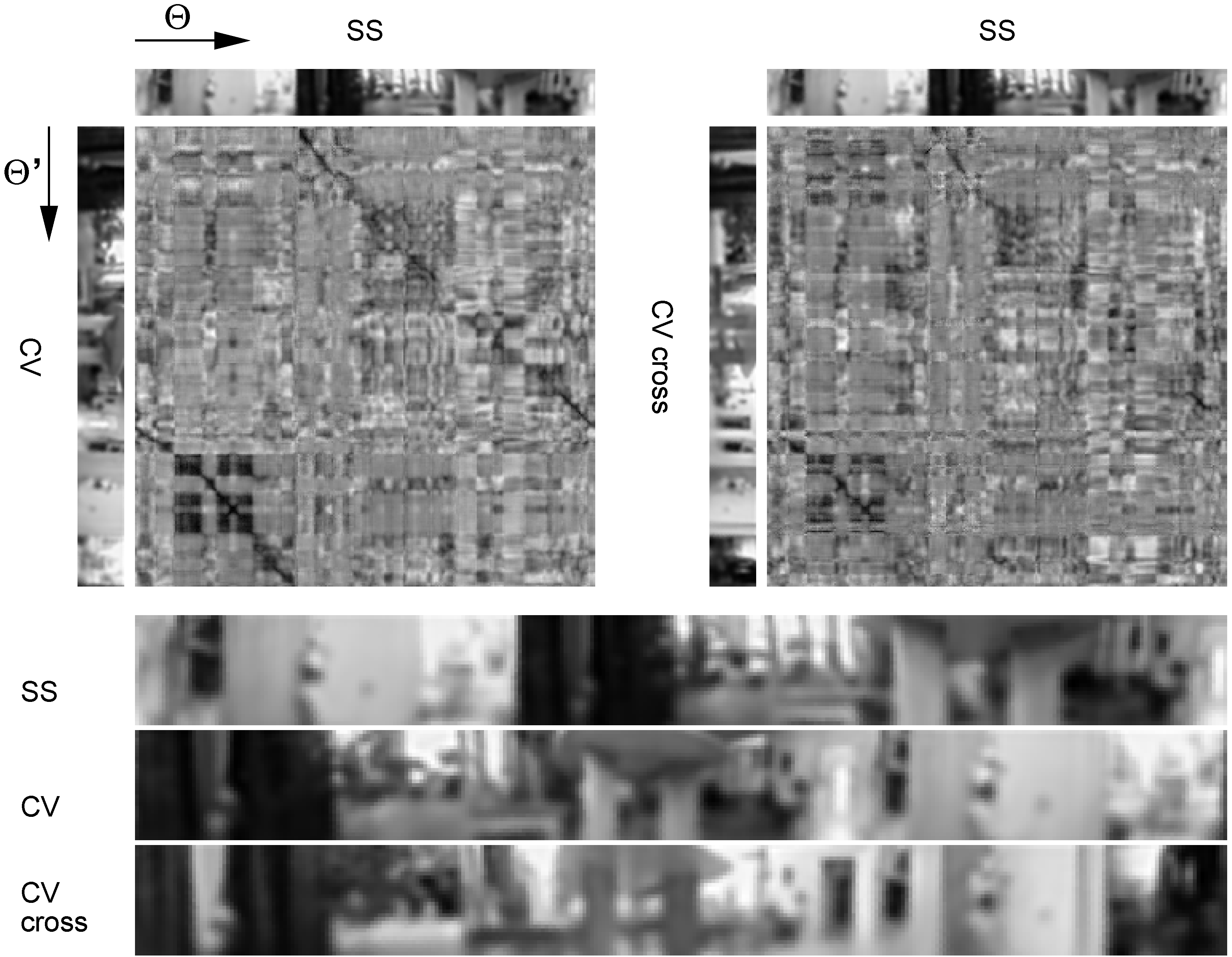
Figure 2. Column distances (square images) computed by J ASC + (Section 3.7) between a panoramic snapshot (SS) and a current view (CV or CV cross) from indoor image databases. Snapshot and current view are taken at different (known) locations (grid positions (6,3) and (4,1) in the living1 databases) and differ in their azimuthal orientation. Darker distance pixels correspond to lower distances. Top left: Snapshot and current view (CV) from the same database (living1day, taken at day). Good matches are easily discernible. Azimuthal angles Θ and Θ are indicated. Top right: Same snapshot, but current view (CV cross) from different image database in the same environment (living1night, taken at night). Good matches are more difficult to see. Bottom: Magnified versions of the snapshot and the two different current views. The current views were taken at the same position but under different conditions of illumination (day, night). Images are shown as they are used by min-warping (low resolution, low-pass filtered).
Robotics 03 00022 g002
For each simulated movement, min-warping searches through all possible locations (azimuthal angle Θ ) where a column in the snapshot (at azimuthal angle Θ) can reappear in the current view and looks for the best match between the snapshot column and the current view column. Even though r and r are unknown, their ratio σ = r / r can be computed from the law of sines in the triangle SCL: σ = ( sin x ) / sin ( x + y ) . The ratio σ is referred to as “scale factor” since it determines how the column in the snapshot should have changed in vertical direction when seen from the current location C, given the movement parameters ( α , ψ ) and the azimuthal angles Θ and Θ under which the column at L appears. Min-warping magnifies one of the columns according to the scale factor and compares it with the other column using some distance measure (the latter being the focus of this paper). The minimal distances (therefore min-warping), obtained from the best matches between columns at given Θ and varying Θ , are summed over all columns Θ of the snapshot and stored in a distance array. Those movement parameters ( α , ψ ) which produce the smallest sum are returned as result. They can directly be converted into the estimates of home vector and visual compass.
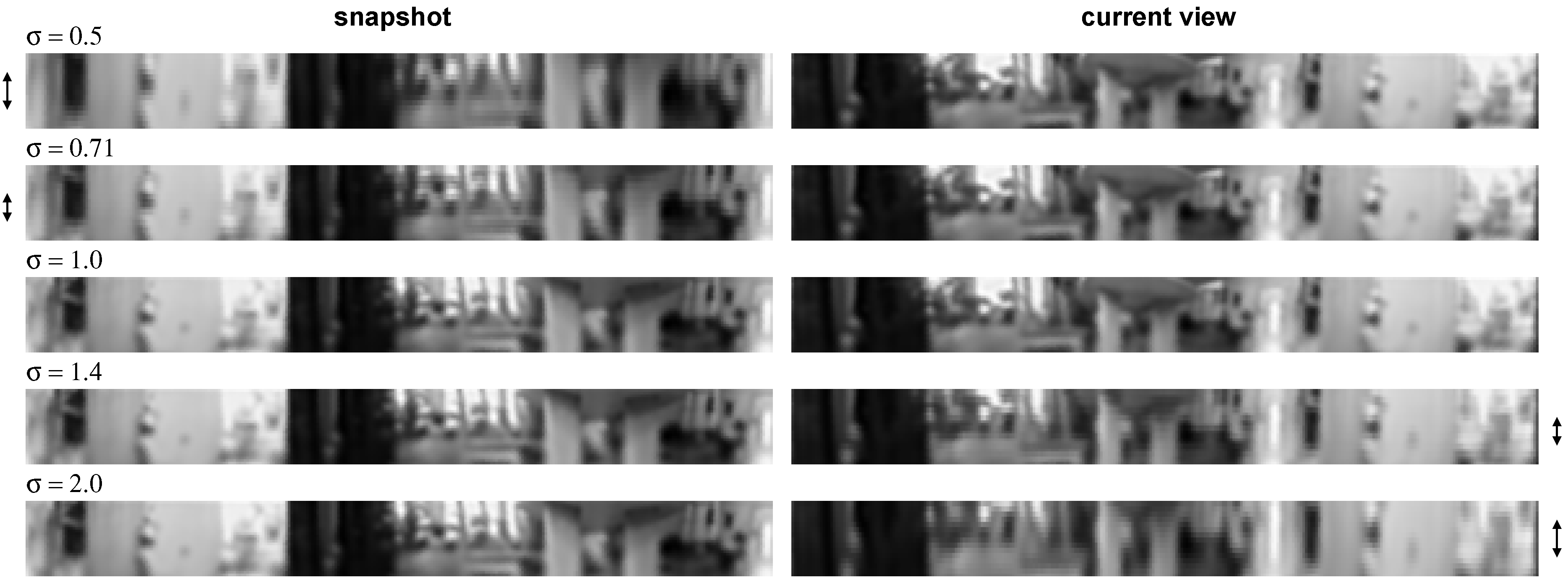
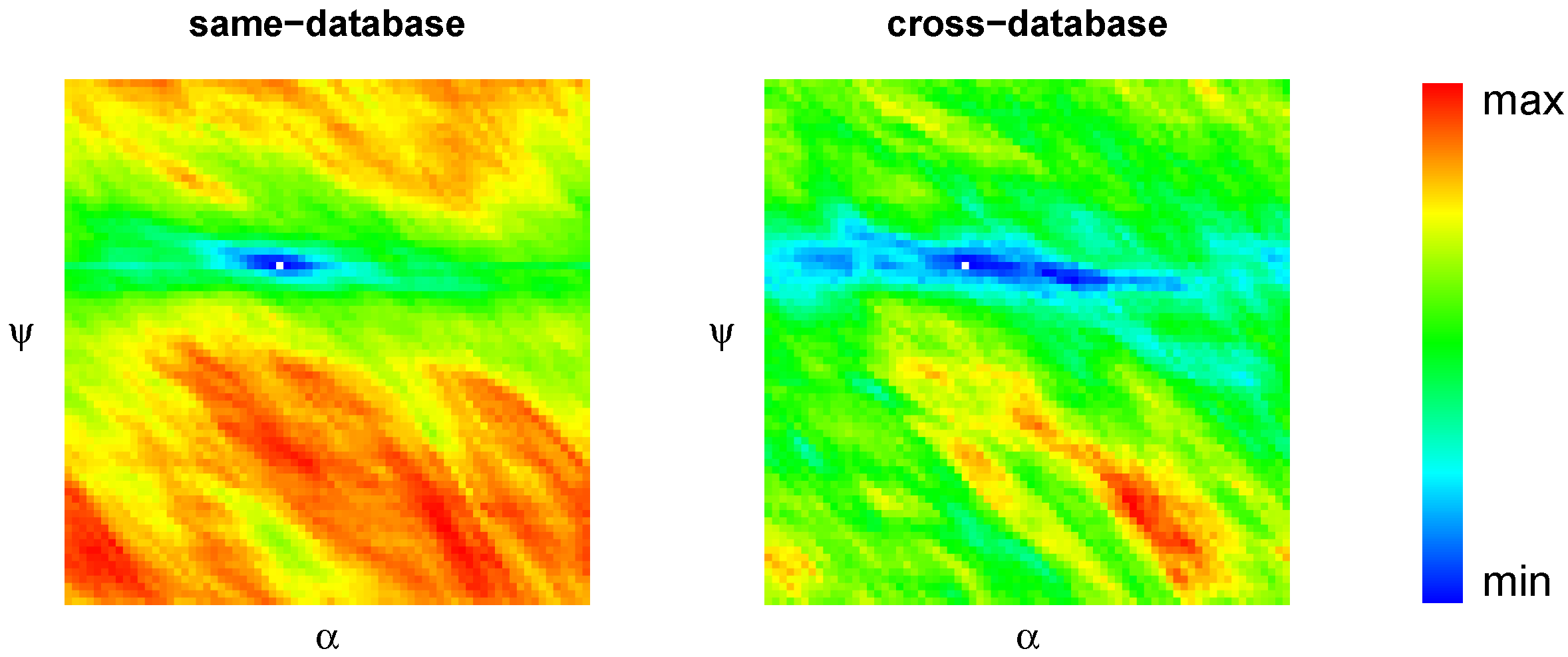
The min-warping algorithm essentially consists of four nested loops through α, ψ, Θ, and a range of Θ (where the range depends on x). However, magnifying and matching image columns in the innermost loop of the min-warping algorithm would be too costly. The algorithm is therefore split into two phases. In the first phase, min-warping precomputes matches between magnified image columns according to a discrete set of scale factors (later, in the second phase, the computed scale factor σ is matched to the closest scale factor from this set). For each scale factor from the set, distances between all image columns in a pair of panoramic images are computed. Figure 2 shows the results of such a distance computation for two images, called snapshot and current view (here used in non-magnified form). The resulting distance image (square image in Figure 2) is referred to as “scale plane”. Figure 3 shows a set of image pairs computed from a set of five scale factors. Computing the distance image between the two images of each pair results in a “scale-plane stack” where multiple scale planes computed over a range of magnification factors are stacked; see Figure 4. In the four nested loops in the second phase of min-warping, distances between a snapshot column and a range of current view columns are obtained from the scale-plane stack. Simulated movement (α, ψ) and azimuthal positions (Θ, Θ ) uniquely determine the scale change σ of an image column such that the scale plane with the nearest magnification factor from the scale-plane stack can be consulted. The result of the second phase is a distance array over the movement parameters ( α , ψ ) ; examples are shown in Figure 5. The white dot in Figure 5 marks the best match (minimum).
Figure 3. Image pairs of snapshot and current view in magnified versions as used in the construction of the scale-plane stack in Figure 4, obtained from the situation shown in Figure 2 (snapshot and current view from same database). The scale factor σ is shown for each image pair. For σ < 1 , the snapshot is magnified (indicated by the arrows), for σ > 1 , the current view is magnified.
Robotics 03 00022 g003
Figure 4. Scale-plane stack obtained from the image pairs in Figure 3. The scale factor σ is shown for each scale plane. Dark values indicate good matches between columns.
Robotics 03 00022 g004
Figure 5. Match-quality arrays for the situation shown in Figure 2. The match quality for each discretized value of the parameters α and ψ (interval [ 0 , 2 π ) , 72 steps) is shown color-coded (blue: good matches). The best match is indicated by a white dot. Left: Same-database test: snapshot and current view from the same database (day). Right: Cross-database test: snapshot and current view from different databases (day/night). Illumination changes in the cross-database test lead to larger uncertainty of the parameter estimates.
Robotics 03 00022 g005
As it is typical for holistic methods, min-warping uses low-resolution input images, and it performs somewhat better if these are slightly low-pass filtered [20,51]. Experiments show that increased image size or inclusion of higher image frequencies have almost no effect on the homing performance (unpublished data). However, using larger images substantially increases the computation time. The computational effort depends on image width w, image height h, number of scale planes n, and number of search parameters n α and n ψ . The effort of the first phase is dominated by a term proportional to n w 2 h , the effort for the second phase is proportional to n α n ψ w 2 / 4 . Doubling image width and height will therefore increase the computation time of the first phase by a factor of 8 and of the second phase by a factor of 4.

1.3. Illumination Invariance and Distance Measures

Illumination changes affect feature-based and holistic methods alike. It is not clear, however, whether methods for achieving illumination tolerance have the same effect on feature-based and holistic methods. The major difference is that feature-based methods only consider high-variance image regions (such as corners) whereas holistic methods consider all parts of an image.
We first look at counter-measures to illumination changes in feature-based methods. In these methods, an image patch is first transformed into an invariant feature descriptor which is then matched by some simpler distance measure (reviews: [1,2,3,4,5,17,18,19]); here the burden of invariance (not only against illumination changes, but also against occlusions, spatial distortions, or noise) is imposed on the transformation. SIFT descriptors [7] comprise summed gradient magnitudes for different orientations in a histogram-like representation. Tolerance against multiplicative illumination changes is achieved by normalizing the feature vector to unit length. Since its entries are derived from images gradients, the feature vector is already tolerant against additive changes. The authors observed that non-linear illumination changes mostly affect the magnitude, not the direction of the gradient vectors, and therefore apply a threshold to all elements of the feature vector and re-normalize. Feature vectors are matched by the Euclidean distance. SURF descriptors [8] are based on Haar wavelets which are tolerant against additive intensity changes. Invariance to multiplicative changes is achieved by normalizing the feature vector to unit length. For matching the descriptors, the Mahalanobis or Euclidean distance is suggested. The original publications on binary feature descriptors [9,10,11,12] remain tacit on how illumination tolerance is achieved. Binary descriptors are bit vectors where each bit encodes whether the intensity difference between two pixels (or regions) of the pair is positive. As long as illumination changes do not affect the sign of the difference, the corresponding bit is unaffected. The selection of the spatial locations of pixels in each pair affect the performance of the predictor, but the publications do not specifically investigate how this selection is related to illumination tolerance. Binary feature vectors are compared by the Hamming distance. The comparative studies in [1,2,5,17] explicitly investigate illumination tolerance (albeit not for the modern binary descriptors).
Holistic methods belong to a wide range of approaches where distance measures (a.k.a. image distance functions or matching costs) are directly computed on intensities or their derivatives (reviews: [60,61,62,63]). Different types of invariance (or at least tolerance), among them invariance against illumination changes, have to be achieved by the distance measure itself. A plethora of such distance measures has been suggested, often with specific applications and specific types of invariance in mind. An extensive review and classification (including a performance comparison) is presented in [61,62]; partial reviews and performance comparisons are provided in [60,63,64,65,66,67]. Chambon and Crouzil [62] provide a helpful classification of distance measures: cross correlation-based methods (“cross”), classical statistics-based measures (“classical”, including distance metrics), derivative-based measures (“derivative”, often based on intensity gradients), non-parametric measures (“non-parametric”, including rank-based measures), and robust measures (“robust”, including median-based measures). An additional class could be introduced which includes histogram-based measures (“histogram”, overview: [68]) including mutual information [66,69].
This paper addresses the question of how to achieve illumination tolerance in the first phase of min-warping where the distances between image columns are computed. This application guides the selection of the distance measures studied here. On the one hand, min-warping works on low-resolution panoramic images where each column typically has only 20–50 elements. On the other hand, the number of comparisons between image columns is large since each column in one image is compared with each column in the other. For images with a width of 360 pixels which are presented in 9 different magnifications [20], 360 2 × 9 1.2 million comparisons between image columns are required. We did not investigate whether it is possible to transform short columns of panoramic images into even shorter feature descriptors to accelerate the large number of matches; instead, we test and develop extremely simple, pixel-wise distance measures. With respect to the classification above, we focus on distance measures directly computed on intensities or their derivatives. All methods studied here belong to the classes “cross” and “classical”. Since min-warping compares vertical image columns and not 2D patches, most measures from the “derivative” class which rely on the direction of intensity gradients cannot be applied. We only explore the effect of a vertical edge filter on measures from “cross”. Measures from the classes “non-parametric” and “robust” have not been studied since we concluded from the results presented below that the additional tolerance introduced by these methods is likely to have a negative effect on the performance of min-warping. The small number of pixels in our application—distance measures are computed between short image columns—also excludes measures from the “histogram” class.
There is currently only one publication which specifically addresses illumination tolerance in holistic local visual homing methods [26]. Stürzl and Zeil investigate how spatial and rotational image distance functions in the DID model are affected by two different ways of preprocessing: DoG filtering and contrast normalization. These are possible alternatives to the edge filtering used in some of our methods, particularly in the novel sequential correlation methods, but so far we have not explored this direction.
Illumination tolerance and tolerance against long-term scene changes is an actively investigated problem in robotics. Even though they are not directly relevant for the work presented in this paper, we point to some recent publications. Our method uses monochrome input, but including color information offers interesting opportunities such as methods for the removal of shadows [70]. Another possible approach to deal with illumination changes is to learn a dictionary of image regions under different conditions of illumination and then transform image regions according to this dictionary before they are matched between images [71]; this may be a possible approach if min-warping is embedded in a more complex localization framework. Some methods are possibly limited to feature-based approaches, such as learning mechanisms where the stability of a feature is determined by integrating multiple observations under different conditions of illumination; in the application phase, only stable (static) features are considered [72]. Also in the context of feature detection, an illumination-invariant difference-of-Gaussians operator for the construction of scalespaces has been introduced [73]; whether a transfer of insights to holistic approaches is possible has to be investigated. Note that some distance measures described in the following appear as components in many computer vision approaches; subtraction of the mean and normalization by the variance of an image patch, for example, has been used for an appearance-based approach to place recognition [74].

1.4. Contributions and Outline of the Paper

This work focuses on tolerance against changes in illumination in min-warping and makes a minor and a major contribution. The minor contribution lies in the development of tunable distance measures. In these distance measures, a portion invariant against multiplicative and/or additive changes in illumination and a portion expressing an overall difference in intensity are superimposed by a weighted average. In experiments on image databases we show that there typically is an optimum of min-warping’s navigation performance for some intermediate weight. One of the tunable measures contains the Euclidean distance (which we have used as distance measure for min-warping before [20]) as a special case. At the optimal weight, the illumination-invariant portion is emphasized compared to the Euclidean distance.
The major contribution of this work are two novel correlation-like measures: “sequential correlation” and a faster form “approximated sequential correlation”. These measures interpret intensities in two vectors as a 2D curve and analyze the direction of curve segments. They are invariant with respect to intensity shifts—in contrast, the well-known normalized cross-correlation is invariant against scaling of intensities, its zero-mean version against scaling and shift. Our experiments show that the performance of sequential correlation is better than that of normalized cross-correlation applied to edge-filtered columns without requiring a second, illumination-sensitive term. A straightforward extension to two-dimensional image patches is described.
Section 2 discusses different types of invariance against shift and scaling of intensities. Section 3 introduces all measures used in this work. Experiments on indoor image databases and their results are presented in Section 4 and Section 5. We discuss the results in Section 6. Section 7 demonstrates that min-warping with the novel approximated sequential correlation measure can be applied to the navigation of cleaning robots. Conclusions from the database experiments are drawn in Section 8.

2. Types of Illumination Invariance

In this section, we introduce different types of invariance against shift and scaling of intensities within an image region (in the case of min-warping: a column of a panoramic image). This allows us to classify the distance measures introduced in Section 3 accordingly. For simplicity, the following discussion assumes a one-dimensional, continuous representation of intensities a ( x ) and b ( x ) in two image regions. A distance measure f { a ( x ) , b ( x ) } computes some (non-negative) integral over these intensity functions. We assume that a perfect match is indicated by a distance measure of zero, i.e., f { a ( x ) , a ( x ) } = 0 .
The methods investigated here establish tolerance against intensity shifts (additive changes) or against intensity scaling (multiplicative changes) over the entire region. In addition, as will be discussed below (Section 6), those distance measures which work on edge-filtered images appear to achieve some kind of local invariance within each image region.
This work deals with two types of invariance against intensity scaling, i.e., against multiplicative changes in intensity. The first type we call weak scale invariance which is achieved if the distance measure exhibits the property
f { c a ( x ) , a ( x ) } = 0
This means that for an arbitrary intensity scaling of an intensity function by a factor c, the distance measure indicates a perfect match with the original intensity function. The second type, strong scale invariance, includes weak scale invariance but in addition ensures that
f { c a ( x ) , b ( x ) } = f { a ( x ) , b ( x ) }
i.e., scaling of one intensity function has no effect on the distance to the other intensity function. This is the stronger type of scale invariance since it not only guarantees that the match of an image region with itself is invariant to scaling, but also that the distance to a different image region is unaffected by scaling. We expect that measures with strong scale invariance will perform better than those with weak scale invariance.
Every distance measure can be made invariant against intensity shifts, i.e., against offsets in intensity. In this work, shift invariance is accomplished by subtracting the mean value or by performing a first-order differentiation before applying the distance measure, or both. If one of the vectors is shifted by an offset c, the distance measure is not affected if the mean is subtracted beforehand,
f { ( a ( x ) + c ) - ( a ¯ + c ) , b ( x ) - b ¯ } = f { a ( x ) - a ¯ , b ( x ) - b ¯ }
or if the distance measure is applied to edge-filtered images,
f d [ a ( x ) + c ] d x , d b ( x ) d x = f d a ( x ) d x , d b ( x ) d x
It is clear that if two intensity functions are scaled versions of each other, i.e., a ( x ) = c b ( x ) , then their derivatives will also be scaled versions of each other
d a ( x ) d x = c d b ( x ) d x
as will be their zero-mean versions,
a ( x ) - a ¯ = c ( b ( x ) - b ¯ )
and the zero mean versions of the derivatives,
d a ( x ) d x - a ¯ = c d b ( x ) d x - b ¯
where a ¯ and b ¯ are the means of the derivatives. Obviously the methods used to introduce additional shift invariance have no effect on scale relationships.
While subtracting the mean removes intensity shifts affecting the entire image region, a first-order differentiation also removes local intensity shifts in sub-regions of constant intensity; only the edge slope between regions of constant intensity is affected. We suppose that this introduces local illumination tolerance (see discussion in Section 6).

3. Distance Measures

In the following subsections we introduce the different distance measures explored in this work. We start with the tunable sum of squared differences since it includes the Euclidean distance—which was originally used by min-warping—as a special case (Section 3.1). A zero-mean version is introduced in Section 3.2. Normalization of the illumination-invariant portion leads to the well-known normalized cross-correlation (Section 3.3). In its tunable form, this measure is combined with the absolute difference of the sum of the intensities; the same illumination-sensitive term is used in all following methods. A zero-mean version of normalized cross-correlation is introduced in Section 3.4. In Section 3.5 we present distance measures where normalized cross-correlation and its zero-mean version are applied to edge-filtered image columns, since also the novel correlation-like measures introduced in this work include an edge filter. Again, tunable versions are defined. We then describe the two novel correlation-like measures introduced in this work, “sequential correlation” (Section 3.6) and its approximated version (Section 3.7), both also available as tunable versions.
In the following we make predictions on the effects of the different distance measures on the performance of min-warping. As performance criterion, we always assume the home vector error as described in Section 4.3.

3.1. Tunable Sum of Squared Differences (TSSD)

In its original form, our visual navigation method “min-warping” computed the Euclidean distance (the square root of the “sum of squared differences”, SSD) between two image columns. The indoor image databases used in the evaluation of the method [20] were collected under constant or moderately varying illumination (mostly caused by changing cloud cover over the day), but not under extreme variations in illumination (like changes between day and night or between natural and artificial illumination). Camera-gain control and histogram equalization were applied to reduce the impact of illumination changes (note that, even under constant illumination, these steps introduce moderate intensity changes as well). Under these conditions, SSD produced robust navigation performance.
Unsurprisingly, as the experiments below will demonstrate, the performance of SSD breaks down under stronger changes in illumination. We therefore first attempt to develop a distance measure which is related to SSD—keeping the good performance under the above-mentioned mild conditions—but which is at the same time tolerant against changes in illumination. For this we assume that changes have a multiplicative effect on the intensities (with intensities being encoded by non-negative values). A distance measure invariant against multiplicative changes should rate the distance between two intensity vectors as minimal (zero) if one is a scaled version of the other.
As shown in Section 2, additional tolerance against additive changes can be achieved by subtracting mean intensities from the intensity vectors. However, it is unclear how this will affect the performance of min-warping: First, invariance against scaling and shift are partly exchangeable—in noisy images it may be difficult to distinguish between moderate scaling and shift. Second, introducing too much tolerance may lead to mismatches. We will explore the influence of double invariance in the experiments.
Applying an illumination-invariant distance measure alone may, however, falsely indicate matches for intensity vectors which are representing different features in the environment and markedly differ in their overall intensity but which nevertheless are scaled (or shifted) versions of each other. While this may occur only rarely in structured image regions, indoor environments often contain uniformly colored walls, curtains, or furniture which can only be distinguished by their overall intensity. Since min-warping does not preselect features (e.g., high-variance regions around corners), ignoring these overall intensity differences may discard information valuable for visual homing. The illumination-invariant measure should therefore be combined with a second, illumination-sensitive measure expressing the difference in the overall intensities of the two image columns. Depending on a weight factor, the influence of both measures can be tuned. We expect that there will be an optimal, intermediate weight factor with respect to the navigation performance.
In the following derivations, the vectors encoding the intensities of the two image columns are denoted by a and b , both of dimension n, with a i 0 and b i 0 . We start with the derivation of the illumination-invariant part of the measure. We suggest a novel form of the “parametric sum of squared differences” (PSSD, see e.g., [64,65]) where the scale parameter γ is split and distributed to both vectors such that the resulting measure is inversion-symmetric (i.e., if a and b are exchanged, the scale factor is inverted but the distance stays the same):
J ˜ PSSD ( a , b , γ ) = 1 2 1 γ a - γ b 2
We determine the optimal value γ ˇ where the distance J ˜ PSSD becomes minimal. It is straightforward to show that the optimal scale factor is
γ ˇ = a b
If we insert γ ˇ into Equation (1) we obtain
J PSSD ( a , b ) = J ˜ PSSD ( a , b , γ ˇ ) = a b - a T b
= a b 1 - a T b a b J NCC
We see from the second Equation (4) that the measure is closely related to the widely used normalized cross-correlation NCC (see e.g., [60,63,64,65]), but leaves out the normalization. J PSSD becomes zero if and only if one intensity vector is a scaled version of the other,
c a a - ( c a ) T a = 0 ,
thus the measure exhibits weak scale invariance; see Section 2. Since
c a b - ( c a ) T b = c ( a b - a T b )
the measure does not exhibit strong scale invariance, though. Since the measure was derived from a quadratic term, it is non-negative. This property is also directly visible from Equation (3) by applying the Cauchy-Schwarz inequality.
For the comparison of the overall intensities we use the squared difference of the length (SDL):
J SDL ( a , b ) = ( a - b ) 2
The combined distance measure, which we call “tunable sum of squared differences” (TSSD), is
J TSSD ( a , b , w ) = w J SDL ( a , b ) + ( 1 - w ) J PSSD ( a , b )
where w is a weight factor from the interval [ 0 , 1 ] . For w = 0 , TSSD only contains the illumination-invariant portion; for w = 1 , it only considers overall intensity differences.
Interestingly, the SSD
J SSD ( a , b ) = a - b 2
is obtained as the special case w = 1 3 of the TSSD in Equation (5) (up to a constant factor),
J TSSD a , b , 1 3 = 1 3 J SSD ( a , b )
The SSD measure can therefore be interpreted as a 2:1 mixture of the fully illumination-invariant PSSD measure and the SDL measure expressing the difference in overall intensities. Reducing the weight w below 1 3 emphasizes the illumination-invariant portion, and we expect an optimal performance of our navigation method in this range. Note that this quantitative interpretation of the weight is only possible for TSSD, not for the other tunable distance measures presented below.
In our implementation of min-warping, we use J TSSD as distance measure to stay close to the Euclidean distance used before (the square root is applied before column distances are summed over the entire image, with the sum indicating the overall match; see [20]).

3.2. Tunable Zero-Mean Sum of Squared Differences (TZSSD)

We also implemented a zero-mean version of TSSD, called TZSSD in the following. Here the illumination-invariant portion J PZSSD is computed for two zero-mean intensity vectors,
J PZSSD ( a , b ) = J PSSD ( a - a ¯ 1 , b - b ¯ 1 )
where a ¯ and b ¯ are the means of the vectors a and b , respectively, and 1 = ( 1 , 1 , , 1 ) T . Since most parts of our implementation of PSSD use unsigned integers, we do not subtract the mean in the beginning, but correct for the mean at later stages in the computation (which is possible by expanding the expression for the zero-mean vectors).
The illumination-sensitive portion is determined from the original intensity vectors, not from the zero-mean versions (since it would otherwise be zero). For this and all following tunable measures we use the absolute difference of sums (ADS) as the illumination-sensitive portion
J ADS ( a , b ) = κ i = 1 n a i - i = 1 n b i
This measure is somewhat easier to compute in an SSE implementation (see Section 4.1) since it doesn’t include multiplications and since we don’t have to take the square root. Moreover, the experiments show that this measure alone ( w = 0 ) works as well as SDL (see Section 5.2). The factor κ results from factors in our integer-based implementation; for input images with pixel range [ 0 , 1 ] it is 1 / 16 for all correlation-type measures and 0.186 for TZSSD.
The TZSSD measure can be written as
J TZSSD ( a , b ) = w J ADS ( a , b ) + ( 1 - w ) J PZSSD ( a , b )
A subtraction of the mean makes the PSSD measure invariant to shifts in illumination (see Section 2). Since PSSD already exhibits (weak) invariance against multiplicative changes in illumination, the resulting measure is invariant against both scaling and shift. We expect a loss of performance compared to TSSD due to an increased portion of false-positive matches as discussed above.

3.3. Tunable Normalized Cross-Correlation (TNCC)

We already saw that PSSD is related to normalized cross-correlation NCC, except for the missing normalization; see Equation (4). In fact, we could derive a form of NCC — here called NCC+ since it only returns positive values from the interval [ 0 , 2 ] — from the distance measure
J ˜ NCC + ( a , b , γ ) = 1 2 1 γ a - γ b 2 a b
We obtain the same optimal value for gamma as in Equation (2), and by inserting the optimal gamma into Equation (6) we get
J NCC + ( a , b ) = 1 - a T b a b J NCC
where the original NCC measure (see e.g., [63]) is underbraced. Alternatively — and this makes the principle underlying this measure more clear —, NCC+ can be written as
J NCC + ( a , b ) = 1 2 J SSSD a a , b b = 1 2 a a - b b 2
where obviously the scaling between the two vectors is eliminated by normalizing them before computing their SSD distance. While normalized cross-correlation can be interpreted as a distance measure, it can also be seen as a transformation (normalization) accomplishing scale invariance followed by a matching using a simpler distance measure, here SSD (for further interpretations of the correlation coefficient, see [75]). NCC+ exhibits strong scale invariance since
1 - ( c a ) T b c a b = 1 - a T b a b
thus we expect a better performance than the PSSD measures.
However, as pointed out by [76], normalization in the presence of noise leads to erroneous estimates for small vectors which may negatively affect the performance. In most feature-matching methods (review: [4]), features to be matched are only extracted at selected key points where the intensities in the neighborhood vary strongly (often corners or scale-space extrema are detected). Normalization is unproblematic in this context as the denominator is far from zero. Min-warping, in contrast, matches all image columns without any selection, thus also image columns with low intensity will be processed by the distance measure. Since the denominator of NCC approaches zero in regions of low intensity, numerical problems may occur and image noise is amplified, adding to the difficulty to make predictions of the performance of NCC+. In our integer-based implementation (using 16 bit unsigned words), we add 1 to the integer denominator to avoid division by zero (if one of the vectors has zero length, a value of J NCC + ( a , 0 ) = 1 is obtained).
For the tunable version, we combine NCC+ with the absolute difference of sums:
J TNCC ( a , b , w ) = w J ADS ( a , b ) + ( 1 - w ) J NCC + ( a , b )

3.4. Tunable Zero-Mean NCC (TZNCC)

We also implemented a zero-mean version of NCC+,
J ZNCC + ( a , b ) = J NCC + ( a - a ¯ 1 , b - b ¯ 1 )
The tunable form is called TZNCC,
J TZNCC ( a , b ) = w J ASC ( a , b ) + ( 1 - w ) J ZNCC + ( a , b )
Here the problem of small denominators is even more severe since it occurs not only for vectors with low intensities, but for all vectors with low variance. This may lead to a performance loss in addition to the problems we expect as a results of the double invariance (see above).

3.5. Tunable NCC on Edge Images (TENCC, TEZNCC)

Edge filtering is integral part of our novel “sequential correlation” methods (Section 3.6 and Section 3.7). For comparison, edge filtering should also be considered as preprocessing step for the standard correlation method (NCC). Since min-warping uses image columns as features, a first-order vertical edge detector is applied (subtraction of the intensities of subsequent, neighboring pixels):
a i = a i + 1 - a i , i = 1 , , n - 1
b i = b i + 1 - b i , i = 1 , , n - 1
We introduce abbreviations for the illumination-invariant terms,
J ENCC + ( a , b ) = J NCC + ( a , b )
J EZNCC + ( a , b ) = J ZNCC + ( a , b )
the bottom one being the zero-mean version, and define the tunable measures TENCC and TZENCC:
J TENCC ( a , b ) = w J ADS ( a , b ) + ( 1 - w ) J ENCC + ( a , b )
J TEZNCC ( a , b ) = w J ADS ( a , b ) + ( 1 - w ) J EZNCC + ( a , b )
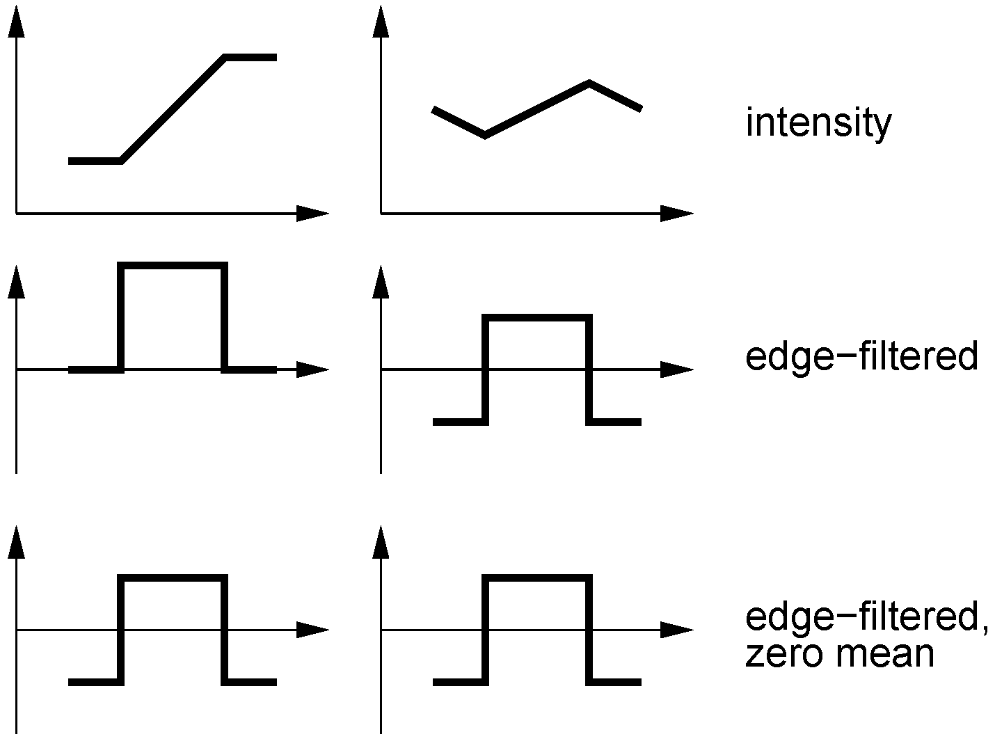
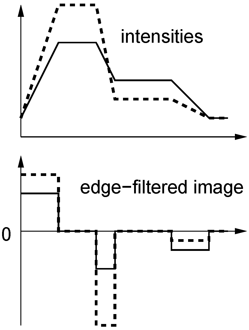
Figure 6. Two identical edge-filtered, zero-mean columns can correspond to widely differing intensity columns.
Robotics 03 00022 g006
The effect of subtracting the mean is difficult to predict. On the one hand, a column of n intensity differences will already have a small mean with a maximal absolute value of a / n if the intensities come from the interval [ 0 , a ] , so any effect should be small. On the other hand, very different intensity vectors can have the same zero-mean edge-filtered version, so there is the danger of mismatches; see Figure 6. We therefore expect a small performance loss if the mean is subtracted.
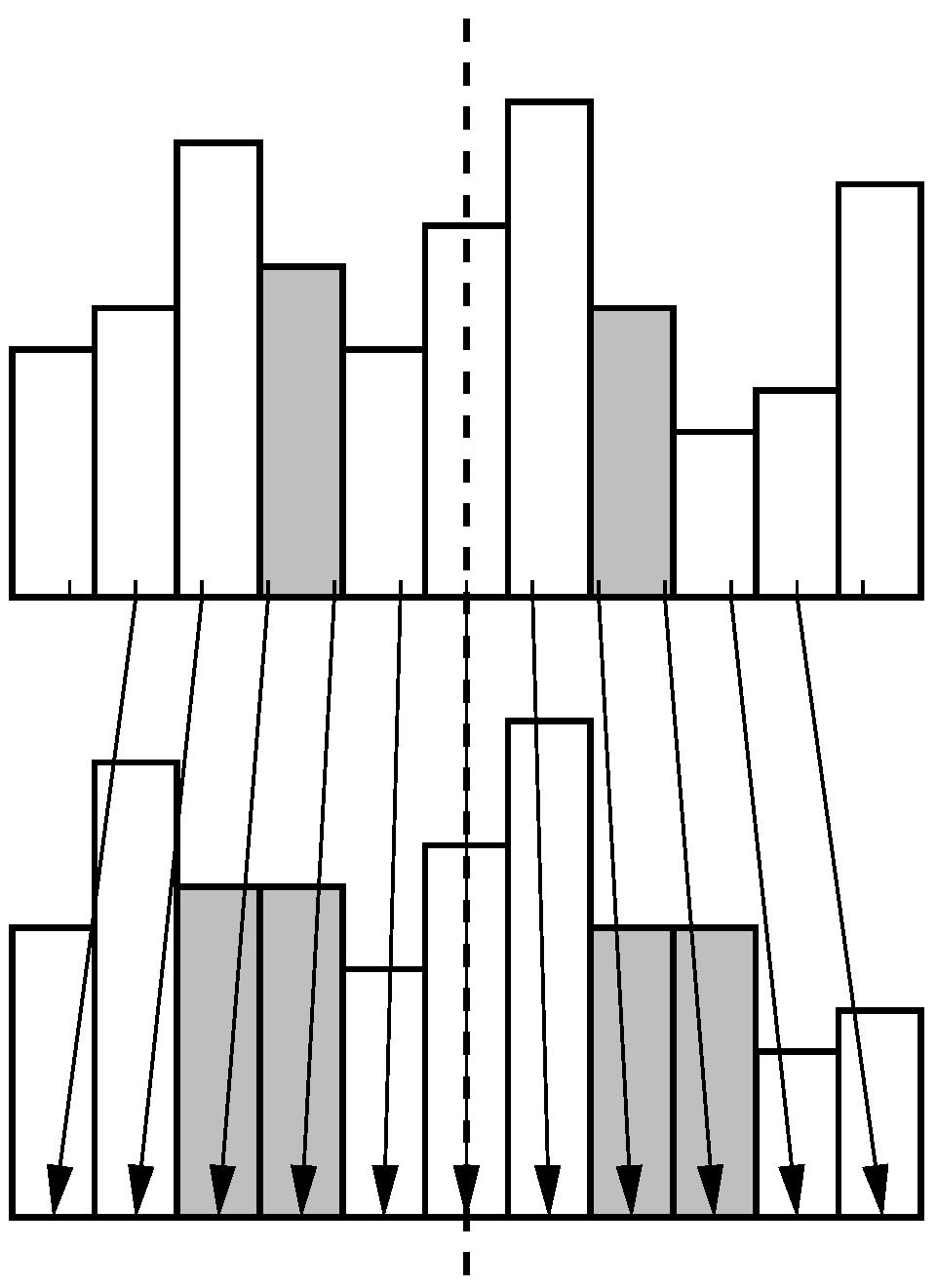
Figure 7. Magnification around the horizon (dashed line) using nearest neighbor interpolation leads to duplicated pixels (gray bars). Intensities in the original (top) and magnified 1D image column (bottom) are shown as bars in order to visualize the nearest-neighbor selection. Arrows indicate the pixel assignment.
Robotics 03 00022 g007
Min-warping does not only compare a single pair of images, but also magnified versions of each image with the original version of the other (see [20]). Magnification only affects the vertical direction and leaves the horizon unchanged. For efficiency reasons, magnification is performed using nearest-neighbor interpolation between image rows which may lead to duplicated image rows, see Figure 7. If a first-order vertical edge filter is applied to a magnified column, erroneous zero entries may be produced. We therefore decided to apply the vertical edge filter to the original two images, and then magnify the edge-filtered image. However, one has to be aware that exchanging the order of the operations affects the result: If an image (for simplicity in continuous representation) is first magnified (M) and then edge-filtered (ME), the derivatives are effectively multiplied by the magnification factor and therefore scaled down (magnification is achieved for 0 < σ < 1 ). Assuming a horizon at x = 0 , this can be written as
f ( x ) f M ( x ) = f ( σ x ) f M E ( x ) = f M ( x ) = σ f ( σ x )
This has to be considered if the image is first edge-filtered (E) and then magnified (EM), since there the derivatives would remain unchanged:
f ( x ) f E ( x ) = f ( x ) f E M ( x ) = f E ( σ x ) = f ( σ x )
Here we have to scale the derivatives by multiplying f E M ( x ) by σ to arrive at the same result as in Equation (7). We will test both versions (with and without scaling of the derivatives).

3.6. Sequential Correlation (SC, TSC)

Sequential correlation and its approximated form (next section) are the major novel contributions of this work. In most of the well-known distance measures like NCC, SSD, PSSD, as well as in the TSSD, TNCC, TZSSD, and TZNCC measures introduced above, the order of the elements in the intensity vectors is of no concern. The fact that the corresponding pixels are adjacent in the image is ignored, and all pixel pairs could as well have been sampled in arbitrary order from the two image columns. For our novel “sequential correlation” measure (SC, or ASC for the approximated version), however, we request that the vectors are ordered such that adjacent elements correspond to adjacent pixels in the image. In natural images, neighboring pixels are known to be strongly correlated, so there is usually a smooth transition of intensities between them, even more so as min-warping prefers slightly low-pass filtered images [20,51]. Please note that the “image Euclidean distance” (IMED) [77,78] was also motivated by the fact that the traditional Euclidean distance ignores the spatial relationship between pixels (leading to large Euclidean distances for small spatial deformations). Interestingly, IMED is equivalent to computing the Euclidean distance on low-pass filtered images [77]. The spatial relationship between pixels is ignored by most other distances measures where a two-dimensional point cloud { ( a i , b i ) } is analyzed, whereas our measures interpret the sequence ( a i , b i ) , i = 1 n as a sampled two-dimensional curve. Essentially, it is a vertical edge filter which introduces the neighborhood relationship between pixels in our novel measures, so the same effect could be achieved by applying other distance measures to edge-filtered images (which we test for normalized cross-correlation; see Section 3.5). Figure 8 (left) visualizes d i .
Figure 8. Visualization of d i used in sequential correlation (left) and of d ^ i used in approximated sequential correlation (right). The zero plane is shown in both plots.
Robotics 03 00022 g008
For the definition of the sequential correlation measure, we start by defining the segment vector between adjacent sequence points,
s i = a i b i = a i + 1 - a i b i + 1 - b i , i = 1 , n - 1
This discrete differentiation step introduces shift invariance; see Section 2. For each segment i of the sequence, we compute the direction term
d i = 2 a i b i s i = s i sin ( 2 α i )
where α i is the orientation of segment i with respect to the a i axis (see Figure 9). The second form shows that (for constant s i ) d i will be maximal for α i = 45 and α i = - 135 (intensity changes in both columns have the same sign and absolute value), and minimal for α i = - 45 and α i = 135 (intensity changes have the same absolute value but different sign). The first form in Equation (8) is used in the implementation (since the second contains a slow trigonometric function). Division by s i may lead to numerical problems (in our integer implementation, where numerator and denominator are integers, we add 1 to the denominator to avoid this), but the second form shows that at least image noise will not be amplified by this normalization.
Using the sums
D = i = 1 n - 1 d i , S = i = 1 n - 1 s i
We define sequential correlation as
J SC = D S [ - 1 , 1 ] , or J SC + = 1 - J SC [ 0 , 2 ]
where the second form is used in our implementation. With the standard correlation coefficient (NCC), J SC shares the range [ - 1 , 1 ] and the symmetry property. SC is invariant against shifts, here achieved by the transition from intensities to intensity differences, but not invariant against scaling. In the integer-based implementation, we add 1 to the denominator to avoid division by zero in Equation (10). We test versions with and without scaling of the derivatives; see Section 3.5. Again, we introduce a tunable form called TSC:
J TSC ( a , b ) = w J ADS ( a , b ) + ( 1 - w ) J SC + ( a , b )
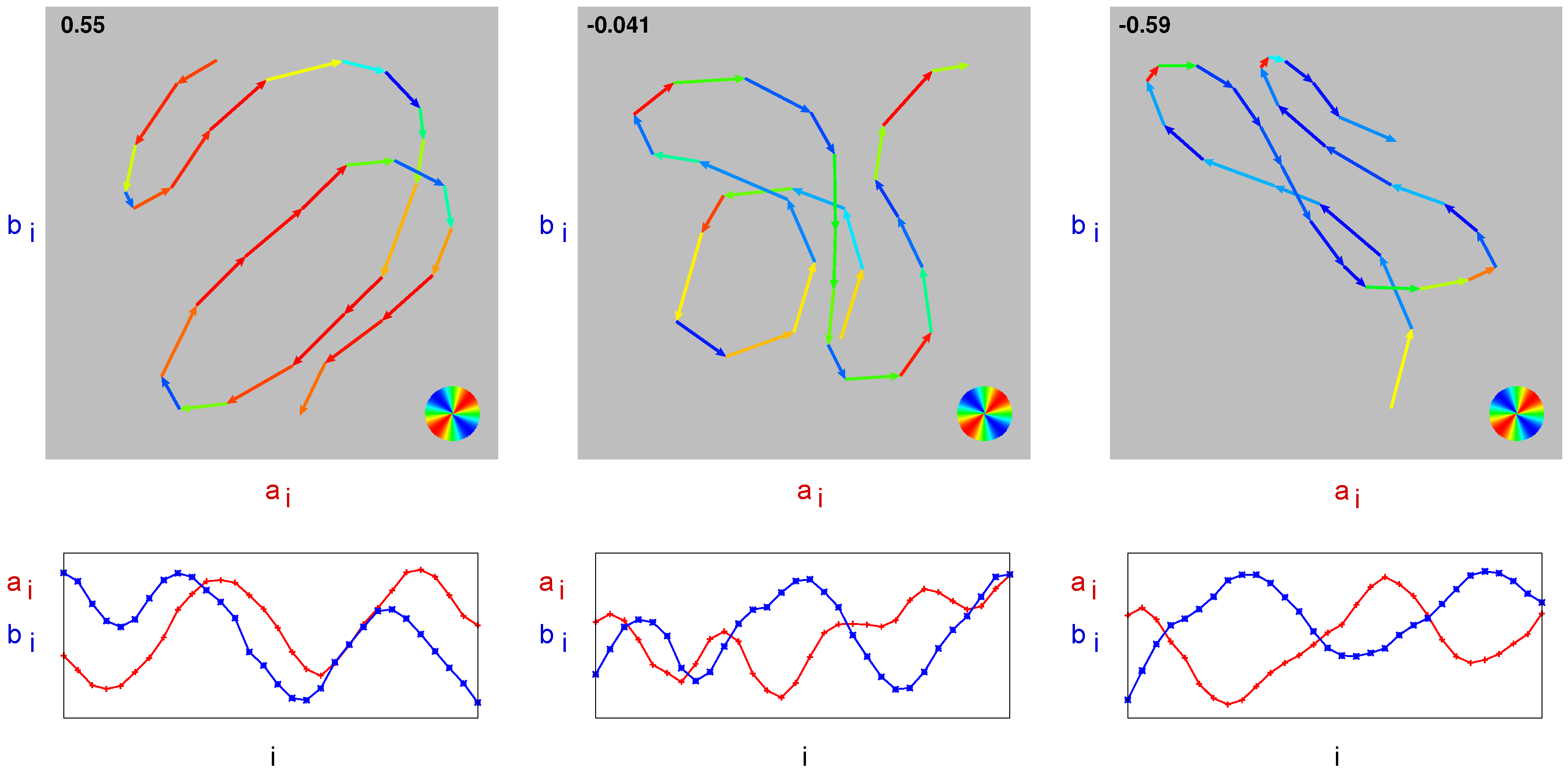
Figure 9. Visualization of sequential correlation. Top row: intensity sequence ( a i , b i ) . Segment vectors are color-coded according to sin ( 2 α i ) (see circle on the bottom right). The value of J SC is given in the upper left corner. Bottom row: corresponding individual intensity curves a i and b i over i. Left column: positive sequential correlation, center column: approximately zero sequential correlation, right column: negative sequential correlation.
Robotics 03 00022 g009
Sequential correlation provides a clear graphical interpretation of correlation on edge-filtered data. In Figure 9 (top row), the intensity sequence ( a i , b i ) is shown for three different examples: positive, approximately zero, and negative sequential correlation. The segment vectors are color-coded according to sin ( 2 α i ) (red + 1 , blue - 1 ). The total length of all segments corresponds to S, the value obtained by summing the product of segment length s i times sin ( 2 α i ) gives D. Their ratio J SC = D / S is specified in the upper left corner.

3.7. Approximated Sequential Correlation (ASC, TASC)

In the implementation of SC, the first form in Equation (8) is used. This computation is, however, awkward due to the square root required to compute the vector length and due to the division. Our implementation uses 16-bit integer arithmetic with eightfold SIMD (single instruction multiple data) parallelity as offered by Intel’s SSE2 instruction set, but parallel versions of square root and division are not available for this format. Since these operations have to be performed for each segment vector s i , the detour via packed floats (4 floats that can be processed in parallel by SSE instructions) results in a marked increase of computation time compared to normalized cross-correlation.
We therefore developed an approximated version of SC, called “approximated sequential correlation” (ASC) which can be implemented almost fully in parallel using just integer instructions. The term d i in Equation (8) was designed such that, for constant s i , it becomes maximal at α i = 45 and α i = - 135 , and minimal at α i = - 45 and α i = 135 ; zero values are achieved for the axis directions ( a i = 0 or b i = 0 ). Moreover, in each direction from the origin, the direction term d i is proportional to s i . A function with the same properties, but with piecewise linear transition is
d ^ i = | a i + b i | - | a i - b i |
see Figure 8 (right). This approximation of d i (up to a constant factor) eliminates square root and division and allows us to implement this computation with eightfold integer parallelity. An equivalent expression is
d ^ i = 2 max { min ( a i , b i ) , - max ( a i , b i ) }
which saves one operation on CPUs which have instructions for maximum and minimum (as is the case for SSE2 instructions on Intel CPUs); note that the factor 2 can be factored out in Equation (13) such that it only has to be applied once per column pair. We define
D ^ = i = 0 n - 1 d i ^ , S ^ = i = 0 n - 1 | a i | + i = 0 n - 1 | b i |
and it can easily be shown by applying the triangle inequality that the measure
J ASC = D ^ S ^
lies within the range [ - 1 , 1 ] . Proof: Triangle inequality: | x + y | | x | + | y | . Therefore i ( | x i + y i | - | x i - y i | ) i ( | x i | + | y i | ) - i | x i - y i | i ( | x i | + | y i | ) which ensures J ASC 1 . Define y i = - y i . Then - i ( | x i + y i | - | x i - y i | ) = i ( | x i + y i | - | x i - y i | ) i ( | x i | + | y i | ) - i | x i - y i | i ( | x i | + | y i | ) = i ( | x i | + | y i | ) which ensures J ASC - 1 .
For our implementation, we use
J ASC + = 1 - J ASC [ 0 , 2 ]
Also ASC is a symmetric measure. As SC, it is only invariant against intensity shifts. An additional advantage is that the two sums of S ^ in Equation (13) can be precomputed individually for each image column whereas S in Equation (9) is inseparable and therefore has to be computed for all column pairs. To avoid division by zero, we add 1 to the denominator in our integer-based implementation of Equation (14). We again test versions with and without scaling of the derivatives; see Section 3.5. The tunable form, TASC, is given by
J TASC ( a , b ) = w J ADS ( a , b ) + ( 1 - w ) J ASC + ( a , b )
While ASC is easier to compute, d ^ i is not continuously differentiable, and closed-form derivations involving ASC would be hampered by the necessary distinction of cases. In SC, d i and s i are continuously differentiable except at a i = b i = 0 , so only this special case has to be handled. So even though SC is computationally more complex, it may still have its value for closed-form derivations, e.g., as a distance measure in gradient or Newton schemes [40,41]. It may then be possible to apply a similar approximation as the one between SC and ASC in the final expressions.

3.8. Correlation Measures on Edge-Filtered Images

It may be helpful to present the equations of all correlation measures on edge-filtered images together and in comparable form:
J NCC ( a , b ) = i a i b i a b
J SC ( a , b ) = 2 i a i b i ( a i , b i ) i ( a i , b i )
J ASC ( a , b ) = i | a i + b i | - | a i - b i | i | a i | + i | b i |
ASC uses an approximation of the numerator of SC, but a different denominator. There cannot be a direct transformation between NCC and SC since NCC is tolerant against scaling and SC is not.

3.9. Correlation of Edge-Filtered 2D Image Patches

In the present form of min-warping, the relations between neighboring columns in the images are not considered since the neighborhood relation changes with the azimuthal distortion of the images and therefore differs between snapshot and current view. Properly including the horizontal interrelations in the search phase would substantially increase the computational effort since optimization techniques like dynamic programming would be required; whether an approximative solution is possible has to be explored. Edge filtering in TENCC/TEZNCC and SC/ASC is therefore only performed in vertical direction within the image columns. For other applications, however, edges can in addition be detected in horizontal direction. Vertical and horizontal differences are simply stacked in a joint vector and compared by the difference measure. An example closely related to min-warping is the visual compass [25,44]. Here entire images—in this case sets of all horizontal and vertical differences—are compared by the difference measure for varying relative azimuthal orientation between the two images. Note that, for correlation-type measures, the normalization here only has to be applied once at the end if the distance measure is applied to the entire image rather than to image columns (which of course gives up local illumination invariance achieved by applying the distance measure individually to each image column as done in min-warping).

4. Experiments

4.1. Implementation

All methods were implemented in C using SSE intrinsics (mostly SSE2) provided by the gcc compiler. SSE intrinsics allow an access to the SSE SIMD machine instructions of the Intel architecture from C. Using these instructions, operations can be performed in parallel on multiple floating point or integer numbers within 128 bit registers. In the largest portion of the code we use eightfold parallelity based on 8 integer words of 16 bit each. Only the vertical edge filtering for the TENCC, TEZNCC, TSC, and TASC is done on float images (input images are provided as float). In SC, the computation of the square root and the division in Equation (8) is done using packed floats (4 floats processed in parallel); this requires two conversion steps between words and floats.
Input images are provided with floating point pixels in the range [ 0 , 1 ] . When the images (or their edge-filtered versions) are converted to word format, pixels are multiplied by a factor. Another factor is used to convert the correlation quotients (range [ 0 , 2 ] ) to words. Both factors are adjusted such that the range of the words (signed or unsigned) is utilized optimally while avoiding overflows.

4.2. Image Databases

Min-warping computes home vectors and compass estimates. All possible applications of min-warping—like following the repeatedly updated home vector to approach a goal location, or triangulating image capture points for navigation in topological-metrical maps [54,55]—depend on the precision of the home vector estimates (note that home vectors depend on both estimated parameters α and ψ). We therefore directly evaluate the precision of home vector estimates using image databases. In each database, panoramic images were captured by placing the robot at known positions on a grid. From this ground truth, true home vector angles can be computed and compared with the home vector angles estimated by the different methods (here min-warping with different distance measures in the first phase); see Section 4.3. The database approach is most suitable for a systematic evaluation of the performance of local visual homing methods since it allows to evaluate thousands of home vector computations (different combinations of snapshots and current views) under controlled conditions such as different conditions of illumination. In our database collection, images were repeatedly captured at the same locations, but under different conditions of illumination. To evaluate illumination tolerance, cross-database experiments can then select snapshot and current view taken under different conditions of illumination.
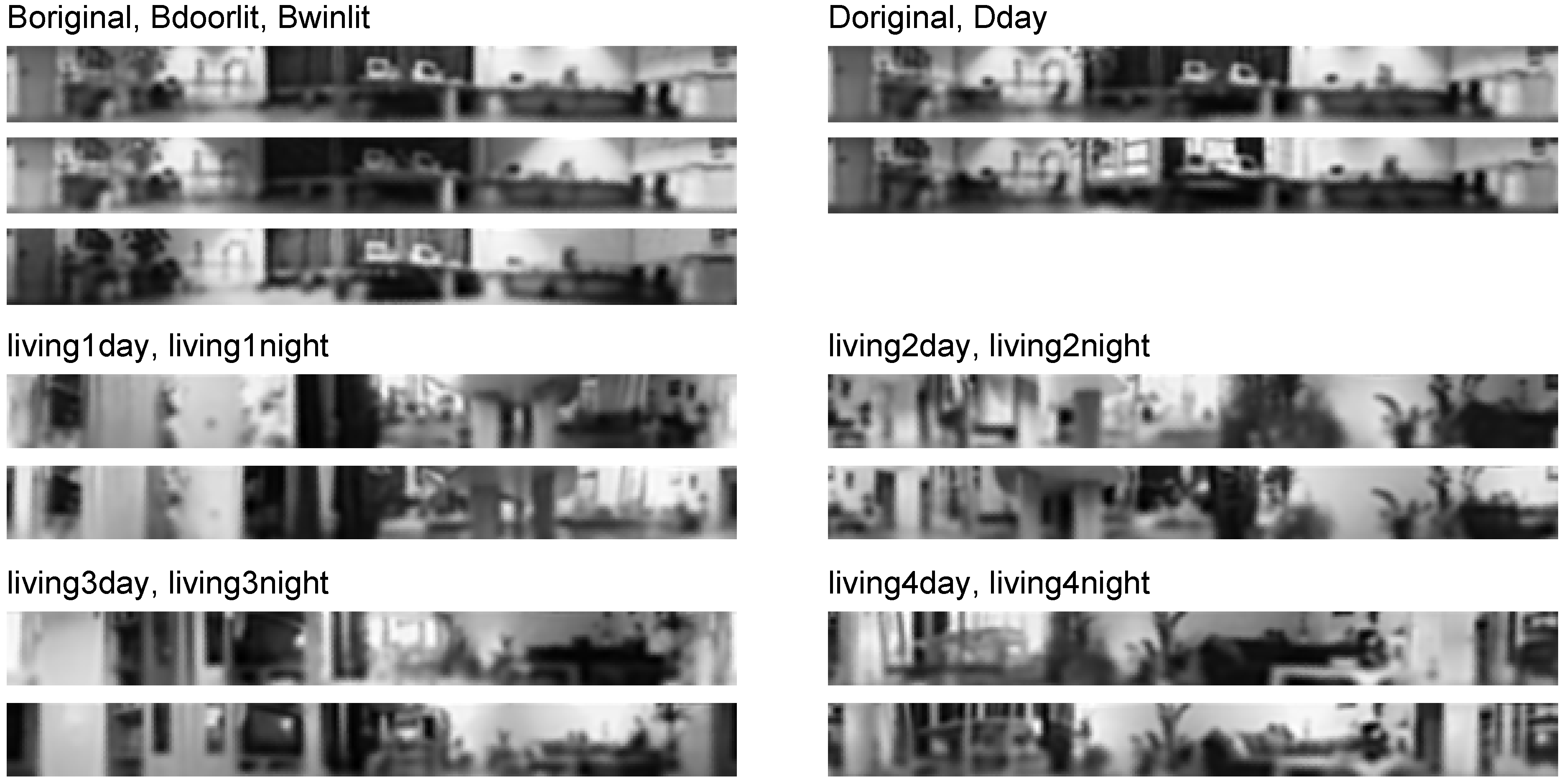
For the experiments, 6 groups of databases were used, see Table 1 and Figure 10; these databases were collected by Andrew Vardy (B*, D*: [79]) and Sven Kreft (living*: [80]). All databases within a group were collected at the same locations but under different conditions of illumination. In the B group of databases, a laboratory room was illuminated from the ceiling lamps, the curtains were closed. In Boriginal, all lamps were on, in Bdoorlit only a row of lamps close to the room’s door side was lit, in Bwinlit only a row of lamps close to the room’s window side was lit. In the D group, the same laboratory room was captured with curtains closed and illumination from the ceiling lamps (Doriginal) and with open curtains at day plus additional illumination from the ceiling lamps (Dday). In the living group of databases, 4 different regions (1–4) of one and the same living room were captured, in each pair during the day and with open curtains (day) and during the night with open curtains and artificial illumination (night). As the experiments show, the changes in illumination are substantial enough (particularly in pairings from the B group and pairings from the living group) to seriously affect the navigation performance of min-warping for some of the distance measures.
Table 1. Image databases used in the experiments: size of the grid, grid spacing in (m) (in parentheses), and image size.
Database GroupGrid Image
Boriginal, Bdoorlit, Bwinlit 10 × 17 ( 0.3 ) 288 × 30
Doriginal, Dday 10 × 17 ( 0.3 ) 288 × 30
living1day, living1night 22 × 4 ( 0.1 ) 288 × 29
living2day, living2night 22 × 5 ( 0.1 ) 288 × 29
living3day, living3night 21 × 7 ( 0.1 ) 288 × 29
living4day, living4night 15 × 3 ( 0.1 ) 288 × 29
For the cross-database experiments, snapshots are taken from one database and current views from a different database from the same group, in that way representing strong changes in illumination. All databases within a group provide the snapshots in turn (leading to 6 pairings in the B group and 2 pairings in all other groups, 16 pairings in total). For the same-database experiments, snapshots and current views are taken from the same database (13 pairings). Since the collection of an image database takes some time, at least in those databases collected at day with open curtains, moderate changes in illumination are possible. Additional changes are introduced by the camera gain control (living databases) and by histogram equalization (used in all databases). From each database pair, 100 randomly selected pairs of snapshots and current views are selected which gives us 1600 home vectors in the cross-database tests and 1300 in the same-database tests. Before being passed to min-warping, both snapshots and current views are rotated randomly in azimuthal direction.
Figure 10. Image databases used in the experiments. An example image from the center of each database is shown as it would be used as input to min-warping (low-pass filtered, histogram-equalized, resolution 1 . 25 deg/pixel). All images are shown in the same azimuthal orientation.
Robotics 03 00022 g010

4.3. Evaluation by Angular Error

For the evaluation of the navigation performance, we use the median and the mean of the angular error (AE, from the interval [ 0 , π ] ) between the computed and the true home-vector direction, the latter being available for all databases since the capture positions (ground truth) of the views are known. From median and mean together we could derive two parameters called “spread” and “error” indicating the precision of the correct home vectors and the portion of erroneous (and therefore uniformly distributed) home vectors, respectively; see [20]. While we do not analyze spread and error here, we nevertheless present both median and mean (always in radians). In most cases there is an optimal weight w of the tunable distance measures in both median and mean; in the few cases where there is no simultaneous optimum for both median and mean, we treat the data point with the optimal median as optimum.

4.4. Statistical Analysis

As in our previous publication [20] we use bootstrapping with B C α correction [81] as the statistical test to compare the median and mean angular error of different distance measures. In each bootstrapping test, the data set comprises angular errors for a pair of distance measures (dependent sample) over all snapshot-current view pairs. This data set is re-sampled 10.000 times. We use a two-sided test with α = 1 % . In the text we specify whether the differences are significant in both median and mean (*), only in the mean (* mean), only in the median (* median), or not significant (n.s.). The results of statistical tests are only presented for the pooled data in the experiments with strong illumination changes.

4.5. Min-Warping Parameters

In all experiments, we use min-warping, one version of warping on two-dimensional images; for the meaning of the following parameters please refer to [20]. We use 9 scale planes (see Figure 2 and Figure 4) for images in different vertical magnification according to scale factors from the set
{ 0.50 , 0.59 , 0.71 , 0.83 , 1.0 , 1.2 , 1.4 , 1.7 , 2.0 }
The thresholds separating the scale-factor ranges are
{ 0.55 , 0.65 , 0.77 , 0.91 , 1.1 , 1.3 , 1.55 , 1.85 , 3.0 }
they define which scale plane is consulted in the search phase. The search range for the two parameters (movement direction α and rotation ψ) spans the entire interval [ 0 , 2 π ) in 72 discrete steps for each parameter. We use a novel version of min-warping (suggested in [82]) with improved performance where the search phase is performed twice, the second time with exchanged images. The stack of scale planes is re-arranged for the second search (a re-computation of the column distances is not required), and the results of the two search phases (match qualities for each parameter combination) are superimposed.
The weight factor w of the tunable distance measures is chosen from the set { 0.0 , 0.01 , 0.02 , 0.03 , 0.04 , 0.06 , 0.08 , 0.1 , 0.2 , 0.333 , 0.4 , 0.5 , 0.7 , 1.0 } for the measures TSSD, TZSSD, TNCC, TZNCC, TENCC, and TEZNCC. For the measures TSC and TASC, we use the following weights { 0.0 , 0.03 , 0.07 , 0.1 , 0.13 , 0.17 , 0.2 , 0.23 , 0.27 , 0.3 , 0.5 , 0.7 , 1.0 } . The weight sets were chosen such that the optimal values of w are covered with sufficient resolution in the diagrams of the median and mean angular error.
All images were low-pass filtered using a Butterworth filter (3rd order, relative cut-off frequency 0.1 ); for details see [51].
In contrast to [20], we don’t use the approximation of image magnification described there in Equation (5), but solve the magnification equation exactly. The vertical resolution of the image (pixels per angle) is required for the exact solution.

5. Results

5.1. Strong Illumination Changes

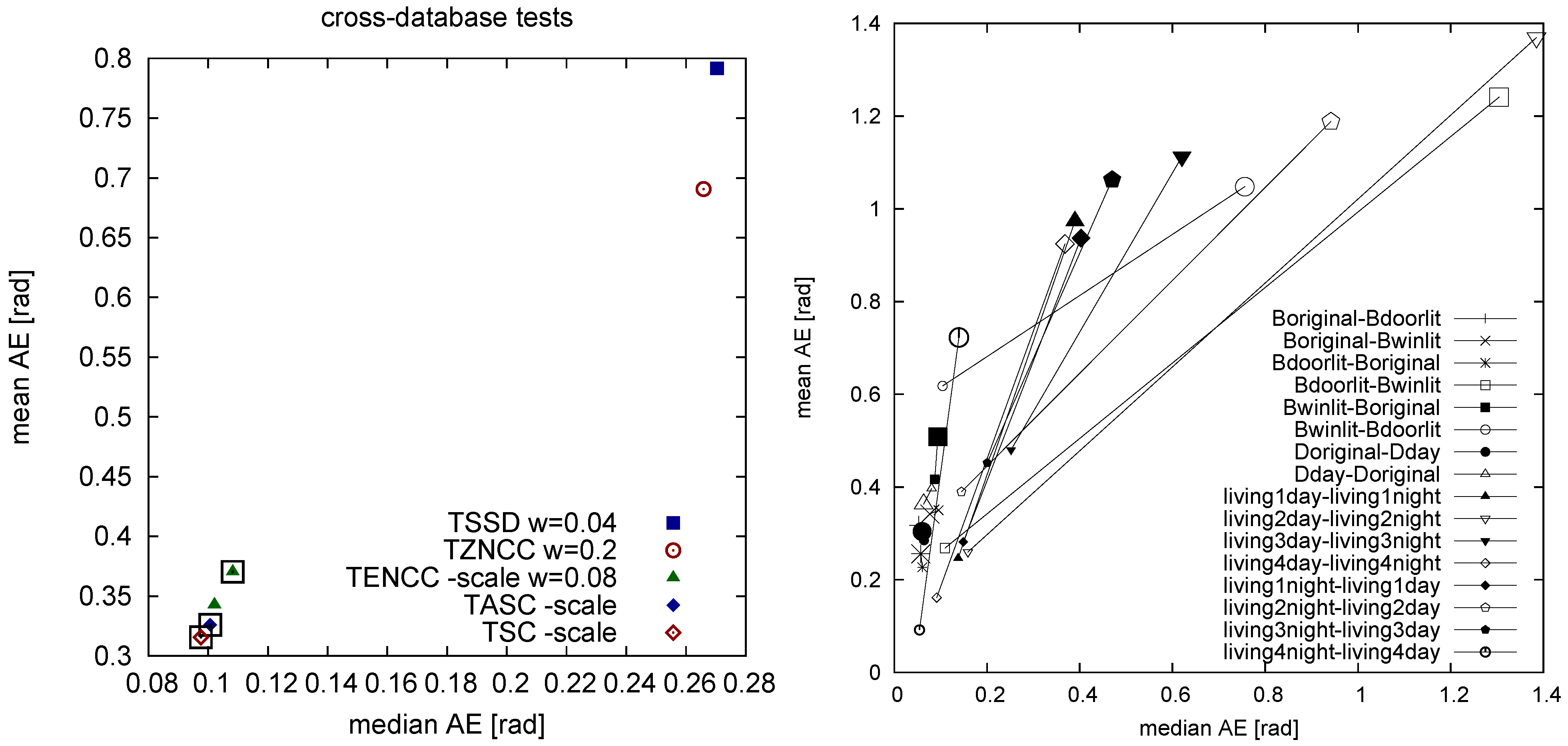
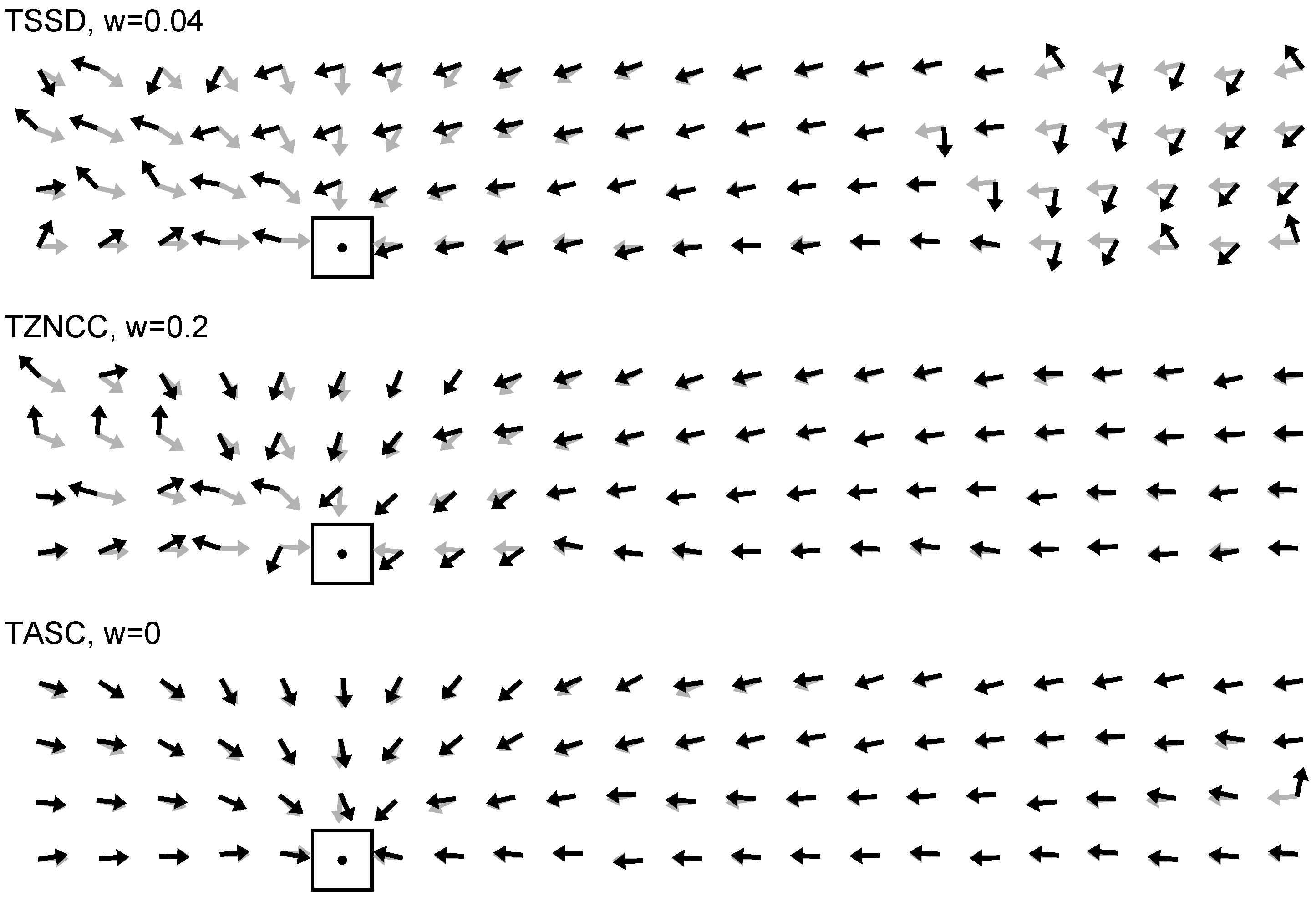
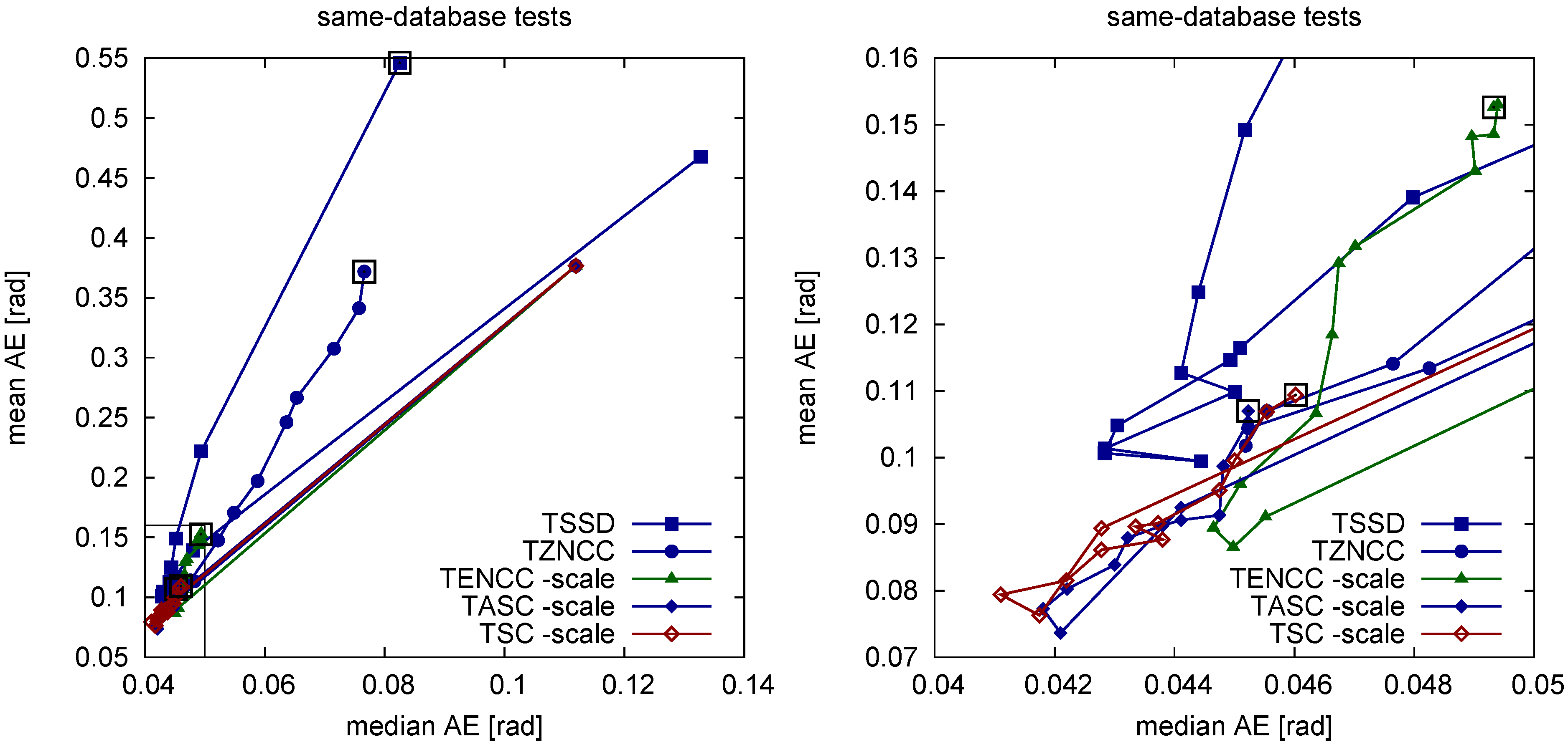
Our objective was to develop distance measures which are tolerant against strong changes in illumination. We therefore analyze results obtained from cross-database experiments in more detail. Figure 11 (left) shows the median and mean angular error for TSSD and TZSSD. The plot confirms our expectation that there is an optimal, intermediate weight w for which the best performance is achieved (TSSD: w = 0.04 ). The optimal performance is much better than both the illumination-invariant portion alone (curve ends marked by large black squares) (*) and the illumination-sensitive portion alone (other curve ends). It is also better than the special case of the Euclidean distance at w = 1 3 (*). Both for w = 0 in both measures (large black squares) and for the optimal w in both measures (data points at the bottom left corner), TSSD performs better than TZSSD (*), thus we can conclude that double invariance (against scale and shift) indeed impairs the performance.
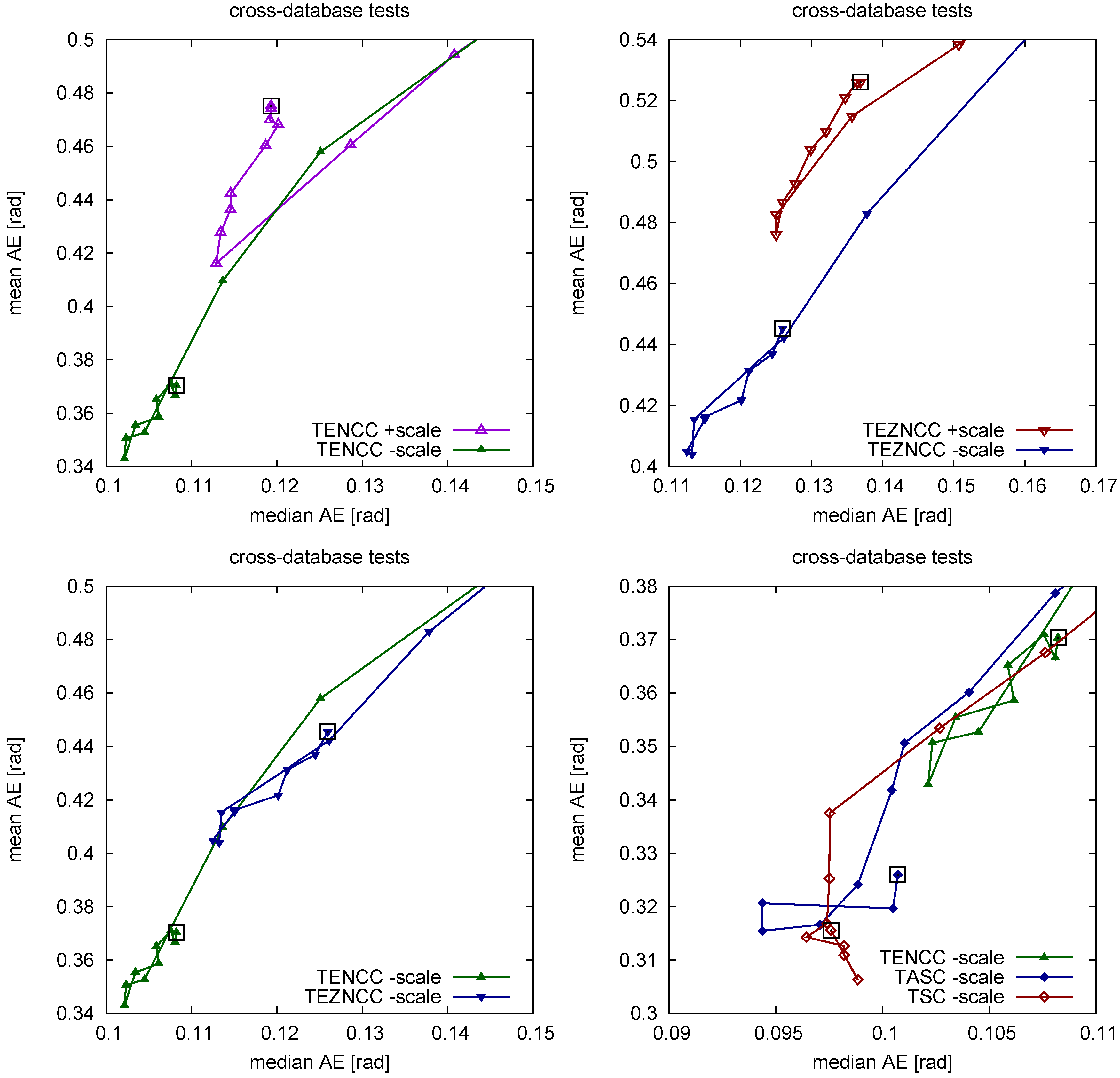
Figure 11. Cross-database tests: Median and mean angular error (radians) for varying w. The larger black squares mark data points for w = 0 . Left: TSSD vs. TZSSD. Right: TNCC vs. TZNCC (only bottom-left region is shown).
Robotics 03 00022 g011
Figure 11 (right) shows a distinct optimum for TZNCC as well ( w = 0.2 ); the performance is better than that of the illumination-invariant term alone (*). However, even though NCC outperforms ZNCC ( w = 0 ) (*)—invariance to scale beats invariance to both scale and shift, and numerical problems with low-variance vectors may affect ZNCC—NCC seems to be incompatible with the illumination-sensitive term: Increasing w leads to worse angular errors. We are fairly sure that this is not a programming error since the code computing the illumination-sensitive term is shared by both measures. At the moment we have no explanation for this effect.
A comparison of the winners TSSD and TZNCC shows that at the best w, TZNCC mostly improves the mean angular error (* mean). This confirms our prediction that methods with strong scale invariance outperform methods with only weak scale invariance (see Section 2).
Figure 12 compares distances measures applied to edge-filtered columns. The top left plot visualizes TENCC. Surprisingly, the correct solution of scaling magnified edge-filtered columns (“+scale”) performs worse than the version were the scaling is not applied (“-scale”), both for w = 0 and for the optimal w in both measures, respectively (*); see Section 3.5. We again see an optimal w, even though the gain compared to the results obtained for w = 0 (large black squares) is relatively small (TENCC+scale: * mean, TENCC-scale: *). Both for w = 0 and for the optimal w, the performance of TENCC-scale is much better than the optimum of TZNCC (*) (see Figure 11; note the different axis ranges), so edge filtering is obviously responsible for the good illumination tolerance. The top right plot compares TEZNCC with and without scaling of the derivatives. Again, the version without scaling performs better, both for w = 0 and for the optimal w (*). The changes over w are comparable to TENCC, and the optima are better than w = 0 (*). The bottom left plot compares TENCC and TEZNCC for the winning versions (without scaling of magnified edge-filtered columns). We see that TENCC outperforms the zero-mean version TEZNCC, both for w = 0 and for the optimal w (*)—again, double invariance doesn’t pay off. For TENCC, the optimum is at w = 0.08 . In the bottom right plot it is visible that the best method from the three other plots, TENCC (without scaling), is outperformed by both TASC and TSC (without scaling), even though the differences are small: TASC ( w = 0 ) is better than TENCC ( w = 0 ) (* mean), but not better than the optimal TENCC (n.s.), and TSC ( w = 0 ) is better than TENCC for w = 0 (*) but not for the optimal w (n.s.). The original version (SC) and the approximated one (ASC) have a similar performance (n.s.). For both, the gain achieved by adding an illumination-sensitive term ( w > 0 ) is so small (TSC: n.s., TASC: * median) that the additional computational effort is wasted. Also for TSC and TASC, the versions without scaling of magnified edge-filtered columns shown in the plot perform better than the versions with scaling, which are not shown (*).
Figure 12. Cross-database tests, see caption of Figure 11. All plots show only the bottom-left regions. Top left: TENCC with (“+scale”) our without scaling (“-scale”) of the magnified edge-filtered columns. Top right: TEZNCC with and without scaling. Bottom left: TENCC vs. TEZNCC (without scaling). Bottom right: TENCC vs. TSC vs. TASC (without scaling).
Robotics 03 00022 g012
Figure 13 (left) compares selected measures from the previous figures. The best performance for TSSD was achieved for w = 0.04 (as expected with a stronger influence of the illumination-invariant portion than in the Euclidean distance, w = 1 3 ), the best performance of TZNCC for w = 0.2 (this value is not interpretable quantitatively). At the optimal weight, TZNCC performs better than TSSD (* mean). However, even for the best w, TZNCC fares very poorly compared to the TENCC measure ( w = 0 and optimal w) which is based on edge-filtered columns (*). Without an additional illumination-sensitive portion ( w = 0 ), the difference between TENCC and TASC/TSC is noticeable, but for the optimal w = 0.08 , TENCC comes close to the performance of our novel correlation measures (statistics see previous paragraph). Edge filtering obviously is a prerequisite for good illumination tolerance. For TASC and TSC we only plotted the version with the illumination-invariant term alone ( w = 0 ) since the gain of adding an illumination-sensitive term was negligible (TSC: n.s., TASC: * median). This is actually an advantage of these methods since there is no need to compute the additional illumination-sensitive term.
Figure 13. Cross-database tests, see caption of Figure 11. Left: Comparison of selected measures (pooled data). Right: Comparison of the navigation performance for cross-database experiments on single database pairs. The first database provides the snapshots, the second the current views. Small symbols: TASC, w = 0 . Large symbols: TSSD, w = 0 . 04 .
Robotics 03 00022 g013
Figure 13 (right) compares the performance of the methods TSSD ( w = 0.04 ) and TASC ( w = 0 )—for which the pooled performance is shown in Figure 13 (left)—for the individual database pairings used in the cross-database experiments. We see a large performance advantage of TASC for most of the database pairs. Only for the pairs Boriginal-Bwinlit and Dday-Doriginal, TASC performs slightly worse than TSSD. TSSD has difficulties with all living databases and with the two pairings of Bdoorlit and Bwinlit, whereas the remaining database pairs show a good performance even for TSSD. We can summarize that the performance differences obtained for the pooled data are also visible for the majority and not only for a small number of database pairs. However, since cross-databases were only available for two types of environments (B*/D*: lab room, living*: living room), we cannot make any claims on applicability to a broader range of environments.
For three of the measures in Figure 13, we show examples of home-vector fields for the database pair living1day/living1night in Figure 14. The differences in performance are clearly visible.
Figure 14. Home-vector fields for cross-database tests with the database pair living1day/living1night. The snapshot was taken at the position marked by the square. Gray vectors indicate perfect home vectors computed from the ground truth, black vectors are computed by min-warping using the different column distance measures.
Robotics 03 00022 g014

5.2. Moderate Illumination Changes

Measures insensitive to strong illumination changes should of course also perform well if the illumination changes are small. Figure 15 compares the performance of selected methods for tests where snapshots and current views were taken from the same database. For all methods, we see pronounced optima for intermediate values of w. As could be expected, the best performance is better than for the strong illumination changes. TSSD achieves the best performance for w = 0.08 0.2 , again below w = 1 3 (Euclidean distance). The magnified bottom-left region (right plot) shows that the optima of all methods are close to each other. Even for w = 0 , TASC and TSC achieve reasonably good performance such that adding the illumination-sensitive term is probably not required. The optima of TASC and TSC are better than all other methods, but they are achieved for high values of w = 0.3 0.5 which are not suitable for strong illumination changes. Values around w = 0.15 appear to be a good compromise working reasonably well both under strong and moderate illumination changes, but we recommend to use w = 0 —the performance gain obtained by including the illumination-sensitive term ( w > 0 ) is so small (for both strong and moderate illumination changes) that the computational effort for this term is not justified.
Figure 15. Same-database tests. Only the best-performing versions (w/o zero mean, w/o scaling) are shown. Left: Entire plot. Right: Bottom-left region (marked in the left plot).
Robotics 03 00022 g015

5.3. Computational Effort

Table Table 2 lists the computation times for the different measures (Intel Core i7-3610QM CPU, 2.30 GHz). The fastest measure is TSSD, but TASC (which exhibits a much better navigation performance in the cross-database tests) is only slightly slower (at least for w = 0 where the illumination-sensitive term is not computed).
Table 2. Average computation times for the different methods (Intel Core i7-3610QM CPU, 2.30GHz). Time 1 is the time for the computation of the illumination-invariant term alone ( w = 0 ), time 2 is the time for the computation of both terms ( w 0 ). In TSSD, both terms are always computed. The second phase of min-warping (search) always takes about 24 ms (full search range, double search; 96 steps of both parameters, used for time measurement only).
MethodTime 1 (ms)Time 2 (ms)
TSSD 3.5 3.5
TZSSD 5.4 7.4
TNCC 6.5 8.4
TZNCC 8.0 9.9
TENCC 6.1 8.1
TEZNCC 6.1 8.1
TASC, Equation (11) 4.5 6.5
TASC, Equation (12) 4.3 6.3
TSC 30.9 32.9
TSC is almost an order of magnitude slower than TASC (and that at comparable navigation performance) which is a result of the square root and division operations required for each segment. All other methods are somewhat slower than TASC (up to a factor of about 2); however, in these cases we did not invest as much effort into speed tuning as in TASC, so there may be more efficient implementations. Computing the illumination-sensitive term (time 2 minus time 1) costs about 2 ms. It may be possible to improve the performance by reducing the number of memory accesses; this could be achieved if the illumination-sensitive term is not computed separately (as done now) but together with the illumination-invariant term. For TASC, we report the computation times for both alternative expressions for d ^ i .

6. Discussion

The results show that tunable distance measures which combine an illumination-invariant and an illumination-sensitive term perform best for a certain mixture of the two measures. The illumination-invariant term alone is obviously not sufficient for min-warping which uses all image columns as features without any selection of key points. Whether a tunable distance measure also has an advantage for methods with feature selection has to be explored. For TSSD we can interpret the optimal mixture weight ( w = 0 . 04 , obtained for strong illumination changes) since we know that w = 1 3 corresponds to the Euclidean distance; compared to the Euclidean distance, the illumination-invariant portion is weighted more strongly. For the other tunable measures we can only say that an intermediate value of w is optimal. TZNCC shows the same behavior (optimum at w = 0 . 2 ), but TNCC seems to be incompatible with the chosen illumination-sensitive term. We didn’t further explore whether another form of illumination-sensitive term would be better suitable since at w = 0 the measure performs much worse than measures working on edge-filtered images. At least for the illumination-invariant portion alone, we always see that introducing additional tolerance against offsets by subtracting the mean leads to impaired performance compared to tolerance against scaling alone. We assume that double invariance introduces false positive matches.
The better performance of TZNCC over TSSD can be explained by the strong vs. weak type of scale invariance. Even though we didn’t test other methods with only weak scale invariance such as the co-linearity criterion suggested by [76] or the image Euclidean distance by [77], we think that they will also be beaten by measures with strong scale invariance.
Figure 16. Effect of edge filtering (bottom) on a 1D intensity image (top) where one region became brighter and another region darker (solid to dashed).
Robotics 03 00022 g016
Edge filtering (here only tested for the correlation-type measures TENCC and TEZNCC) seems to be the best way to achieve tolerance against illumination changes. While NCC on intensities can only remove intensity scaling affecting the entire image region (in our case an image column), edge filtering works locally within the image region: In sub-regions with constant intensity, differences in intensity are completely removed from the image region, even if one part of the region gets brighter and another one darker (and thus scale invariance with respect to the entire region doesn’t help), and intensity changes only affect the slope of the edges (see Figure 16). Still, the slope changes can in principle be strong, and we currently can’t present a mathematical analysis that would show why slope changes should be better tolerated by normalized cross-correlation than changes in the intensity image. Whether the fact that neighborhood relations are considered through edge filtering is an advantage is not clear as well. Note that the good illumination tolerance achieved by edge filtering may be paid for by reduced tolerance against spatial translations in the images [26], e.g., in our example caused by tilt of the robot platform.
If we compare TENCC and TEZNCC, we see that the performance drops if the mean is subtracted, presumably since this step destroys the relation between original and edge-filtered image (very different images can have the same edge-filtered, zero-mean versions, see Figure 6). The optimal weight of TENCC is w = 0 . 08 .
Edge filtering is also the first step of our novel “sequential” correlation measures which treat the two intensity vectors as a sequence of 2D curve points rather than as a mere collection of points without any order. Here the gain achieved by a tunable form is so small that the additional computational effort is not justified. Sequential correlation alone ( w = 0 ) performs best in cross-database experiments (strong illumination changes) and fairly well in same-database experiments (moderate illumination changes). We could show that the performance gain of sequential correlation compared to the best TSSD method which we obtained for the pooled data is also visible for the majority of the individual databases.
We can only guess why the performance of sequential correlation (SC, ASC) is slightly better than the standard normalized cross-correlation on edge-filtered images (TENCC). Normalized cross-correlation is already (strongly) invariant against scaling, and edge filtering introduces additional invariance against shifts. Double invariance impaired the performance for all distance measures applied to the original images (i.e., without edge filtering), at least for w = 0 , presumably due to false positive matches introduced by too much tolerance. In contrast, sequential correlation is only tolerant against shifts—as a result of edge filtering—but not against scaling, which may reduce the number of false positive matches.
At the moment we cannot fully explain the following side observation. There are two ways to perform edge filtering in min-warping: Either an image is magnified (in vertical direction around the horizon) first and then edge-filtered, or it is first edge-filtered and then magnified. Since together with nearest-neighbor interpolation we get erroneous derivatives in the first form, we use the second form in our implementation. To achieve the same effect as in the first form, the edge-filtered image should be scaled down if it is magnified. However, leaving out this scaling operation actually improved the performance in all tested methods. We assume that this version of image magnification fits better with the true magnification resulting from decreasing the spatial distance to the feature. Sharp edges may actually have a similar slope regardless of the spatial distance to the feature, but this explanation needs experimental verification.
At least for a fast, integer-based implementation using SIMD instructions (SSE), the original sequential correlation measure requires considerably more computation time than all other distance measures studied here. We suggested an approximated form which can be computed an order of magnitude faster and which does not differ significantly in the navigation performance. We noticed that, compared to normalized cross-correlation, it was easier to chose the float-to-int conversion factors for approximated sequential correlation in accordance with the upper limits imposed by the integer implementation since the method mostly contains additions, subtractions, and the absolute value function but no multiplication.
Invariance against changes in illumination can be established in multiple ways; Table 3 provides a summary. Weak invariance against scaling can be achieved by finding the optimal scaling such that the distance (e.g., SSD) between two vectors becomes minimal (parametric SSD measures); strong scale invariance is obtained by normalizing the two vectors to the same length before their distance is computed (NCC measures). Invariance against shifts can be obtained by either subtracting the mean from the two vectors before they are compared (zero-mean versions of several measures), or by computing the distance between edge-filtered vectors (NCC on edge-filtered images).
Table 3. Types of invariance of illumination-invariant terms used in the tunable distance measures presented in this work, and navigation performance on databases with strong changes in illumination. Abbreviations: finding the optimal scaling (“scaling”; leads to weak scale invariance), normalizing the vector (“norm”; leads to strong scale invariance), subtracting the mean (“zero-mean”), applying an edge filter (“edge”). The comment “mismatches!” refers to Figure 6.
MeasureScale InvarianceShift InvarianceNavigation Performance
PSSDscaling (weak)
PZSSDscaling (weak)zero-meanworse than PSSD (*)
NCC+norm (strong) better than PSSD (*)
ZNCC+norm (strong)zero-meanworse than NCC+ (*)
ENCC+norm (strong)edgemuch better than NCC+ (*)
EZNCC+norm (strong)edge, zero-meanworse than ENCC+ (*); mismatches!
SC+ edgebetter than ENCC+ (*)
ASC+ edgeclose to SC+ (n.s.)
We can provide the following explanations for the results:
Normalization is better than scaling of vectors. Normalization (NCC+) turned out to be the better way to achieve scale invariance than finding the optimal scaling (PSSD), even though normalization amplifies noise for short vectors. This can be explained by the fact that NCC+ exhibits strong but PSSD only weak scale invariance.
Invariance against both scaling and shift may lead to mismatches. When only the invariant term of the tunable measure was used, combining invariance against scale and shift always resulted in worse navigation performance than using scale invariance alone. We assume that this is due to increased false positive matches introduced by the double invariance.
Subtracting the mean in edge-filtered images may lead to mismatches. Introducing two-fold invariance against shifts by first applying an edge filter and then additionally subtracting the mean may lead to mismatches as visualized in Figure 6.
In NCC+, edge filtering is the best way to achieve shift invariance. Even though NCC+ on edge-filtered images is both scale- and shift-invariant, it performs much better than NCC+ on the original intensity images. Edge filtering seems to introduce some kind of local invariance (see Figure 16) against illumination changes which improves the performance. This is in line with results presented in [83] where it was derived, by using a probabilistic method, that edge information (specifically the gradient direction) is the best way to accomplish illumination invariance (for object recognition).
Sequential correlation performs best since it only relies on edge filtering. Our novel correlation measures (SC+, ASC+) exclusively rely on shift invariance (and there only on edge filtering); this may explain their small performance advantage over NCC+ on edge-filtered images which is invariant against scale and shift. This stands in contrast to feature-based methods such as SIFT or SURF where apparently tolerance against both shift and scaling is beneficial. As NCC+, also SC+ and ASC+ are correlation-type measures with a normalization which may contribute to their good performance. An additional illumination-sensitive term is not required for SC+ and ASC+.
We did not test rank-based distance measures such as Spearman’s rank correlation coefficient [84] which tolerates non-linear illumination changes. Rank-based correlation is not necessarily much more time-consuming since it is applied to each image individually before the two images are interrelated, the latter being the most time-consuming step. However, as we have seen, even simultaneous invariance against both additive and multiplicative changes in intensity resulted in a loss of home vector precision. We therefore expect that the additional tolerance introduced by a rank-based method would further impair the performance.
We also did not test whether a binary representation of each column vector and a distance computation by the Hamming distance as in the BRIEF, ORB, or FREAK descriptors would improve the performance. This would require an optimization process for the selection of pixels pairs within a column from which the binarized intensity difference are computed [9]. It is difficult to predict whether such an approach would improve the performance. Binarizing edge-filtered images (i.e., neighboring pixels form pairs) may impair the performance: Small spatial shifts of the columns introduced by camera tilt would lead to small changes in smooth first derivatives but to larger changes in binarized first derivatives. Binarizing differences between more distant pixels from the column may also not be beneficial: If one part of the column is increased in intensity, local edge filters still recognize the structure in each part whereas differences between more distant pixels may have changed in sign.
All tests described in this paper were performed in two indoor environments, a lab room and a living room, for which cross-illumination databases were available. To the best of our knowledge, there is presently no outdoor image database available where images from the same locations were collected under different conditions of illumination and with sufficiently precise ground truth. We will therefore collect additional cross-illumination databases in indoor and outdoor environments and repeat our tests for these data. For outdoor environments, we have suggested methods where illumination tolerance is achieved by computing contrast measures between UV and visual channels [85,86]; it may improve the performance if the distance measures suggested in this paper are applied to data preprocessed by such contrast methods.
The question whether the results are transferable to other holistic methods, e.g., methods from the DID framework, cannot be answered without systematically investigating these methods. We performed preliminary experiments where we compared the performance of a holistic visual compass method [25] for the TSSD measure ( w = 0 . 04 ) and for the ASC measure. Due to similarities between the first phase of min-warping and the visual compass (see Section 3.3 in [20]), we computed a single scale plane using our min-warping implementation and averaged column distances with the same difference angle Θ - Θ ; the minimal average provides the rotation estimate. Each randomly rotated snapshot was compared to each randomly rotated current view from the same database or from a cross database, using the same databases as for the min-warping experiments. The mean and median angular error between true and estimated azimuthal rotation were computed.
Surprisingly, here the TSSD measure performed better than ASC, both for cross-database and for same-database experiments (see Table 4, first and second row). We can provide the following explanation: Min-warping distorts and rotates one of the input images according to the simulated movement. For the best match, a large portion of pixels belonging to the same point in space will share the same image position with the other image. In contrast, the visual compass only rotates one of the images. Therefore the image distortions caused by the spatial distance between the vantage points are not compensated for, and a larger portion of pixels belonging to the same landmark will not appear at the same image position. Since ASC uses edge-filtered images where low image frequencies have been removed, small distances between pixel locations are sufficient to miss a match between edges. TSSD works on intensities and will therefore tolerate larger distortions. This explanation is in accordance with the observation that rotational image difference functions have very sharp minima if low image frequencies are removed [26]. We expect a similar effect for the DID method where image distortions are not compensated for as well. As a side observation we see from the bottom row in Table 4 that the rotation estimate obtained from min-warping (which considers image distortions) is much better than the rotation estimate obtained from the visual compass (which doesn’t).
Table 4. Mean and median angular error [rad] of the compass estimate (ψ) for cross-database and same-database experiments. The first and second row show the results of the visual compass. For comparison, the bottom row presents the error of min-warping’s compass estimate.
Cross-DatabaseSame-Database
MethodMean AEMedian AEMean AEMedian AE
compass, TSSD ( w = 0.04 )0.770.410.490.24
compass, ASC0.880.480.740.33
min-warping, ASC0.270.040.120.02

7. Application: Cleaning Robot Control

In this section, our intention is not to provide a further test of illumination tolerance, but rather to demonstrate that min-warping with the novel approximated sequential correlation measure can successfully be applied to the control of cleaning robots in unmodified indoor environments. With this we hope to dispel doubts that proponents of feature-based methods may harbor on the general applicability of the holistic min-warping method. This is also one of the first robot experiments we performed where we used approximated sequential correlation in the first phase of min-warping instead of TSSD which was used in [55].
The navigation method used by the cleaning robot is described in detail in [55]. The robot attempts to cover the entire reachable space by adjoining meander parts. On each meander lane, it collects panoramic snapshot images every 10 cm. It then computes home vectors and compass estimates with respect to snapshot images collected on the previous lane of the same meander part or on a previous meander part. Based on these measurements, a particle filter updates the robot’s position estimate, and a controller corrects the movement direction of the robot such that a lane distance of 30 cm is maintained. Each particle cloud associated with a panoramic view can later be used as landmark position estimate. Views and clouds form nodes of a graph-based, topological-metrical map of the environment which is constructed during the cleaning run.
Figure 17. Internal representation obtained in a cleaning run covering three rooms of an apartment (schematic layout is shown in the inset). Target lanes are shown as red lines. Position estimates (averages of particle clouds) are visualized by light blue circles. Parts of the trajectory where the robot traversed existing meander parts to reach the starting point of a new part are omitted for clarity. Black dots are range sensor measurements. The final position of the robot (close to the starting point of the very first lane) is indicated.
Robotics 03 00022 g017
Figure 17 shows the internal representation of the robot’s trajectory for a cleaning run that covers multiple rooms of an apartment. Red lines are target lanes, light blue circles visualize position estimates at all map nodes (averages of particle clouds). It can be seen that a wide portion of the reachable space was covered. (Note that the gap in the range sensor measurements (black dots) close to the robot is actually closed, but the range sensor measurements which originally filled the gap were discarded and could not be replaced by fresh sensor measurements since the robot returned to the start location immediately afterwards and finished the run.) Black dots are range sensor measurements. These are only used to identify uncleaned free space, not for updating the position estimates. Range sensor measurements are attached to the nodes of the topological-metrical map and therefore depend on the position estimates of the corresponding map nodes. When looking at the range sensor measurements it is apparent that even though the map is not fully metrically consistent over several parts, there is not much positional drift within each part—otherwise walls would appear multiple times in the plot. The robot successfully returned to the starting point after finishing the last part (the final position is indicated). Light blue lines depict the snapshot pairings for which min-warping was applied. For each visual correction of the position estimate, typically three home vectors are computed from the current snapshot and three snapshots on the previous lane. The first one, shown in red, points to a snapshot approximately 45 deg from the forward direction, the second one, shown in green, points to the closest snapshot on the previous lane, and the third one, shown in blue, points to the snapshot approximately 45 deg from the backward direction. The quality of the estimates provided by min-warping is apparent from the observation that the home vectors produced by min-warping with ASC almost never switch order (red, green, blue) with respect to their direction and usually correspond well with the estimated direction to the node on the previous lane (light blue). Note, however, that the plots show position estimates, not true positions, and that these position estimates are updated by the same home vectors.
Figure 18 shows all home vectors computed during the cleaning run (compass estimates are omitted for clarity). Figure 19 magnifies the part indicated by the rectangle in Figure 18.
Figure 18. Home vectors (red, green, blue) computed for the update of the position estimate. Light blue lines indicate snapshot pairings from which home vectors (and compass estimates) are computed. The black rectangle indicates the part magnified in Figure 19.
Robotics 03 00022 g018
Figure 19. Magnification of the part enclosed by the black rectangle in Figure 18. Each robot position estimate is shown as a black dot with a black orientation line.
Robotics 03 00022 g019
A quantitative evaluation of the home vectors is not possible without ground truth (which is not available for this run); our intention is just to give a visual impression. We know, however, that metrical consistency within each meander part is usually good enough to judge homing performance from such a visual inspection [55].
Figure 20. Images captured on the center lane and the right lane shown in Figure 19. The images are ordered spatially according to where their corresponding map nodes appear in Figure 19.
Robotics 03 00022 g020
Figure 20 gives a visual impression of the panoramic images (size 320 × 48 ) attached to the map nodes of the center lane and the right lane shown in Figure 19. A red line through the center of each image was added which corresponds to the backward viewing direction of the panoramic camera. Visual features underneath the line shift only by small amounts which indicates that each lane was approximately straight; this corresponds with the position estimates in Figure 19.
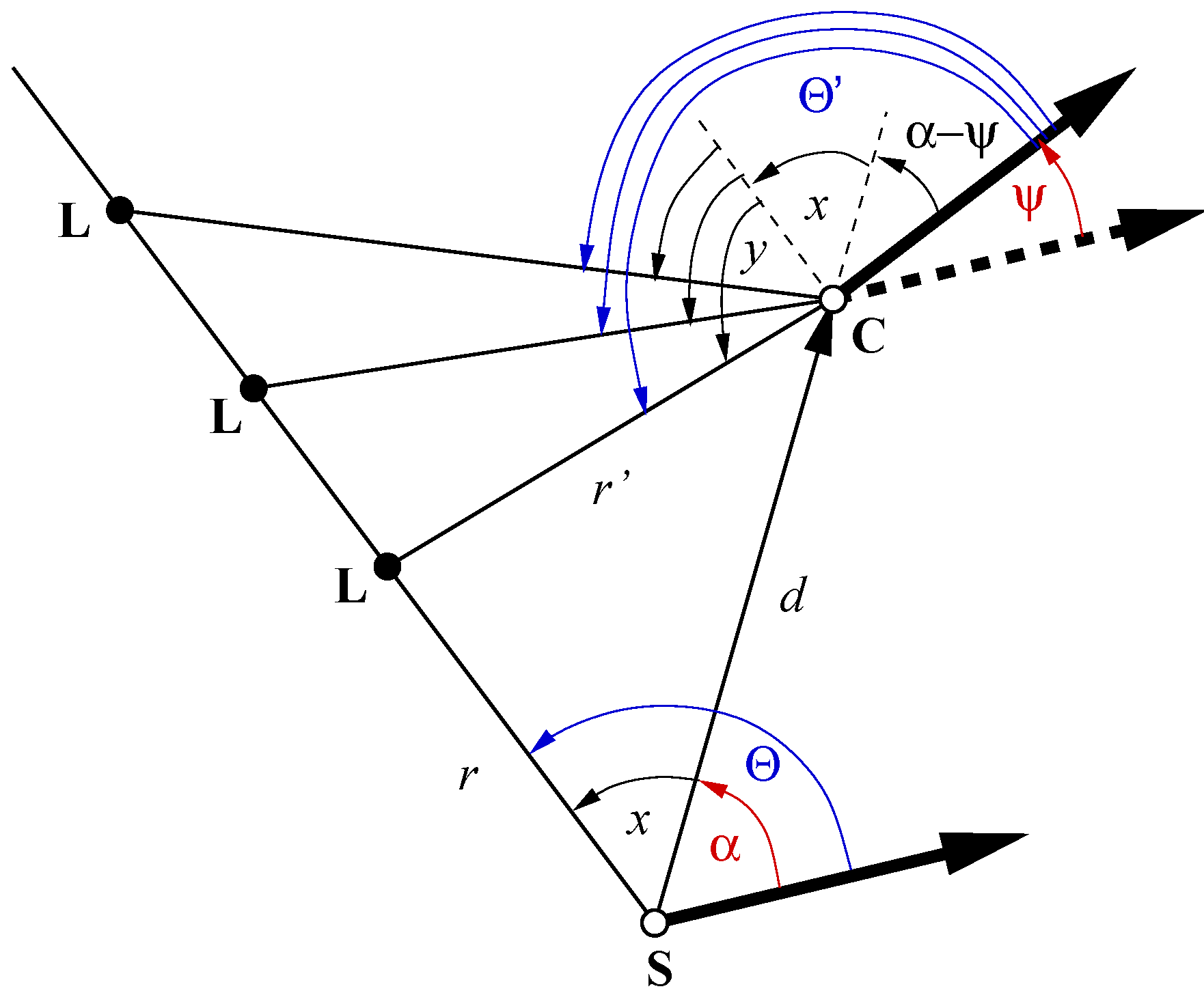
8. Conclusions

The distance measures TSSD, TZSSD, and TZNCC, which work on original (not on edge-filtered) images, profit from a tunable combination of an illumination-invariant and an illumination-sensitive term. In TSSD, this combination is elegant since it contains the Euclidean distance as special case. However, applying distance measures to edge-filtered images leads to a much larger improvement in homing performance, and for these methods, the gain by the weighed superposition with an illumination-sensitive term is relatively small. For TSC and TASC methods introduced in this paper—which perform best among all tested methods—an additional illumination-sensitive term is not required since the resulting performance gain is negligible.
Applying distance methods to edge-filtered images generally leads to good homing performance of the min-warping method. Correlation-based methods exhibit the strong type of scale invariance (TENCC) or are shift-invariant (SC, ASC) and should be preferred. Among these, we can recommend our novel approximated sequential correlation (ASC) measure. The small advantage of ASC over normalized cross-correlation on edge-filtered images can possibly be explained by the fact that ASC is only tolerant against shifts whereas NCC on edge-filtered images is tolerant against both scaling and shifts which may introduce too much tolerance and therefore false positive matches. How ASC performs for holistic methods other than min-warping or for feature-based methods which select high-variance image regions (such as corners) for matching has yet to be explored.

Acknowledgements

We are grateful to Andrew Vardy for his helpful comments on an earlier version of this manuscript. Author Contributions

Author Contributions

Ralf Möller developed and implemented the distances measures and performed the experiments evaluating the home vector quality. Michael Horst and David Fleer integrated min-warping into their framework of cleaning robot navigation and performed the cleaning robot experiments. The paper was written by Ralf Möller.

Conflicts of Interest

The authors declare no conflicts of interest.

References

  1. Mikolajczyk, K.; Schmid, C. A performance evaluation of local descriptors. IEEE Trans. Pattern Anal. Mach. Intell. 2005, 27, 1615–1630. [Google Scholar] [CrossRef] [PubMed]
  2. Mikolajczyk, K.; Tuytelaars, T.; Schmid, C.; Zisserman, A.; Matas, J.; Schaffelitzky, F.; Kadir, T.; van Gool, L. A comparison of affine region detectors. Int. J. Comput. Vis. 2005, 65, 43–72. [Google Scholar] [CrossRef]
  3. Tuytelaars, T.; Mikolajczyk, K. Local invariant feature detectors: A survey. Found. Trends. Comp. Graphics Vis. 2007, 3, 177–280. [Google Scholar] [CrossRef] [Green Version]
  4. Li, J.; Allinson, N.M. A comprehensive review of current local features for computer vision. Neurocomputing 2008, 71, 1771–1787. [Google Scholar] [CrossRef]
  5. Gauglitz, S.; Höllerer, T.; Turk, M. Evaluation of interest point detectors and feature descriptors for visual tracking. Int. J. Comput. Vis. 2011, 94, 335–360. [Google Scholar] [CrossRef]
  6. Rosten, E.; Porter, R.; Drummond, T. Faster and better: A machine learning approach to corner detection. IEEE Trans. Pattern Anal. Mach. Intell. 2010, 32, 105–119. [Google Scholar] [CrossRef] [PubMed]
  7. Lowe, D.G. Distinctive image features from scale-invariant keypoints. Int. J. Comput. Vis. 2004, 60, 91–110. [Google Scholar] [CrossRef]
  8. Bay, H.; Ess, A.; Tuytelaars, T.; van Goal, L. Speeded-up robust features SURF. Comp. Vis. Image Und. 2008, 110, 346–359. [Google Scholar] [CrossRef]
  9. Calonder, M.; Lepetit, V.; Strecha, C.; Fua, P. BRIEF: Binary Robust Independent Elementary Features. In Proceedings of the European Conference Computer Vision (ECCV 10), Crete, Greece, 5–11 September 2010; pp. 778–792.
  10. Calonder, M.; Lepetit, V.; Özuysal, M.; Trzcinski, T.; Strecha, C.; Fua, P. BRIEF: Computing a local binary descriptor very fast. IEEE Trans. Pattern Anal. Mach. Intell. 2012, 34, 1281–1298. [Google Scholar] [CrossRef] [PubMed]
  11. Rublee, E.; Rabaud, V.; Konolige, K.; Bradski, G. ORB: An Efficient Alternative to SIFT or SURF. In Proceedings of the IEEE International Conference Computer Vision (ICCV 11), Barcelona, Spain, 5–11 November 2011; pp. 2564–2571.
  12. Alahi, A.; Ortiz, R.; Vandergheynst, P. FREAK: Fast Retina Keypoint. In Proceedings of the IEEE Conference Computer Vision and Pattern Recognition (CVPR 12), Providence, RI, USA, 16–21 June 2012; pp. 510–517.
  13. Scaramuzza, D.; Fraundorfer, F. Visual odometry. Part I: The first 30 years and fundamentals. IEEE Robot. Autom. Mag. 2011, 18, 80–92. [Google Scholar]
  14. Fraundorfer, F.; Scaramuzza, D. Visual odometry. Part II: Matching, robustness, optimization, and applications. IEEE Robot. Autom. Mag. 2012, 19, 78–90. [Google Scholar]
  15. Lemaire, T.; Lacroix, S. SLAM with panoramic vision. J. Field Rob. 2007, 24, 91–111. [Google Scholar] [CrossRef]
  16. Gamallo, C.; Mucientes, M.; Regueiro, C. Visual FastSLAM through Omnivision. In Proceedings of the Towards Autonomous Robotic Systems (TAROS 09), Derry, UK, 12–14 September 2009; pp. 128–135.
  17. Gil, A.; Martinez Mozos, O.; Ballesta, M.; Reinoso, O. A comparative evaluation of interest point detectors and local descriptors for visual SLAM. Mach. Vis. Appl. 2010, 21, 905–920. [Google Scholar] [CrossRef] [Green Version]
  18. Schmidt, A.; Kraft, M.; Fularz, M.; Domagała, Z. Comparative assessment of point feature detectors and descriptors in the context of robot navigation. J. Autom. Mob. Rob. Intell. Syst. 2013, 7, 11–20. [Google Scholar]
  19. Valgren, C.; Lilienthal, A.J. SIFT, SURF & seasons: Appearance-based long-term localization in outdoor environments. Rob. Auton. Syst. 2010, 58, 149–156. [Google Scholar]
  20. Möller, R.; Krzykawski, M.; Gerstmayr, L. Three 2D-warping schemes for visual robot navigation. Auton. Robot. 2010, 29, 253–291. [Google Scholar] [CrossRef]
  21. Möller, R. A model of ant navigation based on visual prediction. J. Theor. Biol. 2012, 305, 118–130. [Google Scholar] [CrossRef] [PubMed]
  22. Zeil, J. Visual homing: An insect perspective. Curr. Opin. Neurobiol. 2012, 22, 285–293. [Google Scholar] [CrossRef] [PubMed]
  23. Collett, M.; Chittka, L.; Collett, T.S. Spatial memory in insect navigation. Curr. Biol. 2013, 23, R789–R800. [Google Scholar] [CrossRef] [PubMed]
  24. Möller, R. Do insects use templates or parameters for landmark navigation? J. Theor. Biol. 2001, 210, 33–45. [Google Scholar] [CrossRef] [PubMed]
  25. Zeil, J.; Hoffmann, M.I.; Chahl, J.S. Catchment areas of panoramic images in outdoor scenes. J. Opt. Soc. Am. A 2003, 20, 450–469. [Google Scholar] [CrossRef]
  26. Stürzl, W.; Zeil, J. Depth, contrast and view-based homing in outdoor scenes. Biol. Cybern. 2007, 96, 519–531. [Google Scholar] [CrossRef] [PubMed]
  27. Basten, K.; Mallot, H.A. Simulated visual homing in desert ant natural environments: Efficiency of skyline cues. Biol. Cybern. 2010, 102, 413–425. [Google Scholar] [CrossRef] [PubMed]
  28. Graham, P.; Philippides, A.; Baddeley, B. Animal cognition: Multi-modal interactions in ant learning. Curr. Biol. 2010, 20, R639–R640. [Google Scholar] [CrossRef] [PubMed]
  29. Baddeley, B.; Graham, P.; Phillipides, A.; Husbands, P. Holistic visual encoding of ant-like routes: Navigation without waypoints. Adapt. Behav. 2011, 19, 3–15. [Google Scholar] [CrossRef]
  30. Baddeley, B.; Graham, P.; Husbands, P.; Phillipides, A. A model of ant route navigation driven by scene familiarity. PLoS Comput. Biol. 2012. [Google Scholar] [CrossRef] [PubMed]
  31. Lambrinos, D. Navigation in Biorobotic Agents. Ph.D. Thesis, Department of Computer Science, University of Zurich, Zurich, Switzerland, 1999. [Google Scholar]
  32. Lambrinos, D.; Möller, R.; Labhart, T.; Pfeifer, R.; Wehner, R. A mobile robot employing insect strategies for navigation. Rob. Auton. Syst. Spec. Issue: Biomim. Robot. 2000, 30, 39–64. [Google Scholar] [CrossRef]
  33. Möller, R. Insect visual homing strategies in a robot with analog processing. Biol. Cybern. 2000, 83, 231–243. [Google Scholar] [CrossRef] [PubMed]
  34. Mangan, M.; Webb, B. Modelling place memory in crickets. Biol. Cybern. 2009, 101, 307–323. [Google Scholar] [CrossRef] [PubMed]
  35. Gerstmayr-Hillen, L.; Schlüter, O.; Krzykawski, M.; Möller, R. Parsimonious Loop-Closure Detection Based on Global Image-Descriptors of Panoramic Images. In Proceedings of the IEEE Xplore 15th International Conference Advanced Robotics (ICAR), Sarajevo, Bosnia, 20–23 June 2011; pp. 576–581.
  36. Hillen, L. From Local Visual Homing Towards Navigation of Autonomous Cleaning Robots. Ph.D. Thesis, Bielefeld University, Bielefeld, Germany, 2013. [Google Scholar]
  37. Stürzl, W.; Cheung, A.; Cheng, K.; Zeil, J. The information content of panoramic images I: The rotational errors and the similarity of views in rectangular experimental arenas. J. Exp. Psychol. Anim. B 2008, 34, 1–14. [Google Scholar] [CrossRef] [PubMed]
  38. Cheung, A.; Stürzl, W.; Zeil, J.; Cheng, K. The information content of panoramic images II: View-based navigation in nonrectangular experimental arenas. J. Exp. Psychol. Anim. B. 2008, 34, 15–30. [Google Scholar] [CrossRef] [PubMed]
  39. Arena, P.; de Fiore, S.; Fortuna, L.; Nicolosi, L.; Patené, L.; Vagliasindi, G. Visual homing: Eperimental Results on an Autonomous Robot. In Proceedings of the IEEE Xplore 18th European Conference on Circuit Theory and Design, Sevilla, Spain, 26–30 August 2007; pp. 304–307.
  40. Möller, R.; Vardy, A. Local visual homing by matched-filter descent in image distances. Biol. Cybern. 2006, 95, 413–430. [Google Scholar] [CrossRef] [PubMed]
  41. Möller, R.; Vardy, A.; Kreft, S.; Ruwisch, S. Visual homing in environments with anisotropic landmark distribution. Auton. Robot. 2007, 23, 231–245. [Google Scholar] [CrossRef]
  42. Labrosse, F. Short and long-range visual navigation using warped panoramic images. Rob. Auton. Syst. 2007, 55, 675–684. [Google Scholar] [CrossRef] [Green Version]
  43. Pajdla, T.; Hlaváč, V. Zero Phase Representations of Panoramic Image for Image Based Localization. In Proceedings of the 8th International Conference Computer Analysis of Images and Patterns, Ljubljana, Slovenia, 2–5 September 1999; pp. 550–557.
  44. Labrosse, F. The visual compass: Performance and limitations of an appearance-based method. J. Field Rob. 2006, 23, 913–941. [Google Scholar] [CrossRef] [Green Version]
  45. Stürzl, W.; Möller, R. An Insect-Inspired Active Vision Approach for Orientation Estimation with Panoramic Images. In Bio-inspired Modeling of Cognitive Tasks; Springer: Berlin, Germany, 2007; Volume 4527, pp. 61–70. [Google Scholar]
  46. Saez Pons, J.; Hübner, W.; Dahmen, H.; Mallot, H.A. Vision-Based Robotic Homing in Dynamic Environments. In Proceedings of the 13th IASTED International Conference Robotics and Applications, Wuerzburg, Germany, 15–17 June 2007; pp. 293–298.
  47. Zhang, A.M.; Kleeman, L. Robust appearance based visual route following for navigation in large-scale outdoor environments. Int. J. Rob. Res. 2009, 28, 331–356. [Google Scholar] [CrossRef]
  48. Franz, M.O.; Schölkopf, B.; Mallot, H.A.; Bülthoff, H.H. Where did I take that snapshot? Scene-based homing by image matching. Biol. Cybern. 1998, 79, 191–202. [Google Scholar]
  49. Stürzl, W.; Mallot, H.A. Efficient visual homing based on Fourier transformed panoramic images. Rob. Auton. Syst. 2006, 54, 300–313. [Google Scholar] [CrossRef]
  50. Franz, M.O.; Stürzl, W.; Hübner, W.; Mallot, H.A. A Robot System for Biomimetic Navigation—From Snapshots to Metric Embeddings of View Graphs. In Robotics and Cognitive Approaches to Spatial Mapping; Jefferies, M.E., Yeap, W.K., Eds.; Springer: Berlin, Germany, 2008; Chapter 14; pp. 297–314. [Google Scholar]
  51. Möller, R. Local visual homing by warping of two-dimensional images. Rob. Auton. Syst. 2009, 57, 87–101. [Google Scholar] [CrossRef]
  52. Franz, M.O.; Schölkopf, B.; Mallot, H.A.; Bülthoff, H.H. Learning view graphs for robot navigation. Auton. Robot. 1998, 5, 111–125. [Google Scholar] [CrossRef]
  53. Hübner, W.; Mallot, H.A. Metric embedding of view-graphs—a vision and odometry-based approach to cognitive mapping. Auton. Robot. 2007, 23, 183–196. [Google Scholar] [CrossRef]
  54. Gerstmayr-Hillen, L.; Röben, F.; Krzykawski, M.; Kreft, S.; Venjakob, D.; Möller, R. Dense topological maps and partial pose estimation for visual control of an autonomous cleaning robot. Rob. Auton. Syst. 2013, 61, 497–516. [Google Scholar] [CrossRef]
  55. Möller, R.; Krzykawski, M.; Gerstmayr-Hillen, L.; Horst, M.; Fleer, D.; de Jong, J. Cleaning robot navigation using panoramic views and particle clouds as landmarks. Rob. Auton. Syst. 2013, 61, 1415–1439. [Google Scholar] [CrossRef]
  56. Narendra, A.; Gourmaud, S.; Zeil, J. Mapping the navigation knowledge of individually foraging ants, Myrmecia croslandi. Proc. R. Soc. B 2013, 280, 20130683. [Google Scholar] [CrossRef] [PubMed]
  57. Scaramuzza, D.; Fraundorfer, F.; Pollefeys, M. Closing the loop in appearance-guided omnidirectional visual odometry by using vocabulary trees. Rob. Auton. Syst. 2010, 58, 820–827. [Google Scholar] [CrossRef]
  58. Milford, M. Vision-based place recognition: How low can you go? Int. J. Rob. Res. 2013, 32, 766–789. [Google Scholar] [CrossRef]
  59. Schatz, A. Visuelle Navigation mit “Scale Invariant Feature Transform”. Diploma Thesis, Faculty of Technology, Bielefeld University, Bielefeld, Germany, 2006. [Google Scholar]
  60. Aschwanden, P.; Guggenbühl, W. Experimental Results from A Comparative Study on Correlation-Type Registration Algorithms. In Robust Computer Vision: Quality of Vision Algorithms; Förstner, W., Ruwiedel, S., Eds.; Wichmann: Karlsruhe, Germany, 1992; pp. 268–288. [Google Scholar]
  61. Chambon, S.; Crouzil, A. Dense Matching Using Correlation: New Measures That are Robust near Occlusions. In Proceedings of the British Machine Vision Conference, Norwich, UK, 8–11 September 2003; pp. 15.1–15.10.
  62. Chambon, S.; Crouzil, A. Similarity measures for image matching despite occlusions in stereo vision. Pattern Recognit. 2011, 44, 2063–2075. [Google Scholar] [CrossRef]
  63. Giachetti, A. Matching techniques to compute image motion. Image Vis. Comput. 2000, 18, 247–260. [Google Scholar] [CrossRef] [Green Version]
  64. Pan, B. Recent progress in digital image correlation. Exp. Mech. 2011, 51, 1223–1235. [Google Scholar] [CrossRef]
  65. Pan, B.; Xie, H.; Wang, Z. Equivalence of digital image correlation criteria for pattern matching. Appl. Opt. 2010, 49, 5501–5509. [Google Scholar] [CrossRef] [PubMed]
  66. Hirschmüller, H. Evaluation of stereo matching costs on images with radiometric differences. IEEE Trans. Pattern Anal. Mach. Intell. 2009, 31, 1582–1599. [Google Scholar] [CrossRef] [PubMed]
  67. Tombari, F.; di Stefano, L.; Mattoccia, S.; Galanti, A. Performance Evaluation of Robust Matching Measures. VISAPP 2008. In Proceedings of the 3rd International Conference Computer Vision Theory and Applications, Madeira, Portugal, 22–28 January 2008; pp. 473–478.
  68. Rubner, Y.; Tomasi, C.; Guibas, L.J. The earth mover’s distance as a metric for image retrieval. Int. J. Comput. Vis. 2000, 40, 99–121. [Google Scholar] [CrossRef]
  69. Viola, P.; Wells, W.M. Alignment by maximization of mutual information. Int. J. Comput. Vis. 1997, 24, 137–154. [Google Scholar] [CrossRef]
  70. Corke, P.; Paul, R.; Churchill, W.; Newman, P. Dealing with Shadows: Capturing Intrinsic Scene Appearance for Image-Based Outdoor Localisation. In Proceedings of the IEEE/RSJ International Conference Intelligent Robots and Systems (IROS), Tokyo, Japan, 3–8 November 2013; pp. 2085–2092.
  71. Sünderhauf, N.; Neubert, P.; Protzel, P. Predicting the Change—A Step towards Life-Long Operation in Everyday Environments. In Proceedings of the Robotics Challenges and Vision Workshop, Berlin, Germany, 24–28 June 2013.
  72. Johns, E.; Yang, G.Z. Dynamic Scene Models for Incremental, Long-Term, Appearance-Based Navigation. In Proceedings of the IEEE International Conference Robotics and Automation (ICRA), Karlsruhe, Germany; 2013; pp. 2731–2736. [Google Scholar]
  73. Vonikakis, V.; Chrysostomou, D.; Kouskouridas, R.; Gasteratos, A. A biologically inspired scale-space for illumination-invariant feature detection. Meas. Sci. Technol. 2013, 24, 074024. [Google Scholar] [CrossRef]
  74. Milford, M.; Vig, E.; Scheirer, W.; Cox, D. Towards Condition-Invariant, Top-Down Visual Place Recognition. In Proceedings of the Australasian Conference Robotics and Automation, Sydney, Australia, 2–4 December 2013.
  75. Rodgers, J.L.; Nicewander, W.A. Thirteen ways to look at the correlation coefficient. Am. Stat. 1988, 42, 59–66. [Google Scholar] [CrossRef]
  76. Mester, R.; Aach, T.; Dümbgen, L. Illumination-Invariant Change Detection Using a Statistical Colinearity Criterion. In Proceedings of the Pattern Recognition, 23rd DAGM-Symposium, Munich, Germany, 12–14 September 2001; Volume 2191, pp. 170–177.
  77. Wang, L.; Zhang, Y.; Feng, J. On the Euclidean distance of images. IEEE Trans. Pattern Anal. Mach. Intell. 2005, 27, 1334–1339. [Google Scholar] [CrossRef] [PubMed]
  78. Li, J.; Lu, B.L. An adaptive image Euclidean distance. Pattern Recognit. 2009, 42, 349–357. [Google Scholar] [CrossRef]
  79. Vardy, A. Biologically Plausible Methods for Robot Visual Homing. Ph.D. Thesis, Carleton University, Carleton, Canada, 2005. [Google Scholar]
  80. Kreft, S. Reinigungstrajektorien Mobiler Roboter unter Visueller Steuerung. Diploma Thesis, Faculty of Technology, Bielefeld University, Bielefeld, Germany, 2007. [Google Scholar]
  81. Efron, B.; Tibshirani, R.J. An Introduction to the Bootstrap; CRC: New York, NY, USA, 1998. [Google Scholar]
  82. Gedicke, T. Warping for 3D Laser Scans. Bachelor’s Thesis, University of Osnabrück, Osnabrück, Germany, 2012. [Google Scholar]
  83. Chen, H.F.; Belhumeur, P.N.; Jacobs, D.W. In search of Illumination Invariants. In Proceedings of the IEEE Conference Computer Vision and Pattern Recognition CVPR’00, Graz, Austria, 7–13 May 2000; Volume 1, pp. 254–261.
  84. Spearman, C. The proof and measurement of association between two things. Am. J. Psychol. 1904, 15, 72–101. [Google Scholar] [CrossRef]
  85. Möller, R. Insects could exploit UV-green contrast for landmark navigation. J. Theor. Biol. 2002, 214, 619–631. [Google Scholar] [CrossRef] [PubMed]
  86. Kollmeier, T.; Röben, F.; Schenck, W.; Möller, R. Spectral contrasts for landmark navigation. J. Opt. Soc. Am. A 2007, 24, 1–10. [Google Scholar] [CrossRef]