An Improved Reinforcement Learning System Using Affective Factors

Abstract

As a powerful and intelligent machine learning method, reinforcement learning (RL) has been widely used in many fields such as game theory, adaptive control, multi-agent system, nonlinear forecasting, and so on. The main contribution of this technique is its exploration and exploitation approaches to find the optimal solution or semi-optimal solution of goal-directed problems. However, when RL is applied to multi-agent systems (MASs), problems such as “curse of dimension”, “perceptual aliasing problem”, and uncertainty of the environment constitute high hurdles to RL. Meanwhile, although RL is inspired by behavioral psychology and reward/punishment from the environment is used, higher mental factors such as affects, emotions, and motivations are rarely adopted in the learning procedure of RL. In this paper, to challenge agents learning in MASs, we propose a computational motivation function, which adopts two principle affective factors “Arousal” and “Pleasure” of Russell’s circumplex model of affects, to improve the learning performance of a conventional RL algorithm named Q-learning (QL). Compared with the conventional QL, computer simulations of pursuit problems with static and dynamic preys were carried out, and the results showed that the proposed method results in agents having a faster and more stable learning performance.

1. Introduction

“Reinforcement” is first used by Pavlov in his famous conditioned reflex theory of the 1920s. It explains that the stimulus from the external environment can be categorized as rewards or punishments and they change the nature of the brain and the behavior of animals. The concept of reinforcement has been introduced in artificial intelligence (AI) from the 1950s and, as a bio-inspired machine learning method, reinforcement learning (RL) has been developed rapidly since the 1980s [1]. As analyzed by Doya, RL may take place in the basal ganglia of the brain: even the parameters used in RL may involve neuromodulators such as dopamine, serotonin, noradrenaline and acetylcholine [2]. In recent years, RL has been widely used in game theory [1], autonomous robotics [3,4], intelligent control [5,6], nonlinear forecasting [7,8,9,10], multi-agent systems (MASs) [11,12,13,14,15,16,17,18], and so on.

In [3], Asada et al. proposed a vision-based RL method to acquire cooperative behaviors of mobile robots in dynamically changing real worlds. In [4], Kollar and Roy combined RL with extended Kalman filter (EKF) to realize trajectory optimization of autonomous mobile robots in an unknown environment. Jouffe proposed a fuzzy inference system with RL to solve nonlinear control problems in [5], meanwhile Obayashi et al. realized robust RL for control systems adopting slide mode control concept in [6]. In our previous works, several kinds of neuro-fuzzy network types RL systems have been proposed as the time series predictors [7,8,9,10], and the internal models of agents to solve the goal-directed exploration problems in unknown environments [11,12,13,14]. Kobayashi et al. adopted attention degree into an RL named Q learning (QL) for multi-agent system (MAS) [15,16,17] acquiring adaptive cooperative behaviors of agents and confirmed the effectiveness of their improved RL by simulations of the pursuit problem (hunting game) [18].

The principle of RL can be summarized as using the adaptive state-action pairs to realize the optimal state transition process where optimal solution means that the maximum rewards are obtained by the minimum costs. The rewards from the environment are changed to be the values of states, actions, or state-action pairs in RL. Almost all well-known RL methods [1,19,20,21,22] use the value functions to change the states of the learner to find the optimized state transitions. However, when the learner (agent) observes the state of environment partially or the state of the environment is uncertain, it is difficult to select adaptive actions (behaviors). For example, in a multi-agent system (MAS), i.e., multiple agents exploring an unknown environment, neighborhood information is dynamic and the action decision needs to be given dynamically, the autonomy of agents makes the state of the environment uncertain and not completely observable [11,12,13,14,15,16,17,18]. When RL is applied to MASs, problems such as “curse of dimension” (the explosion of state-action space), “perceptual aliasing problem” (such as the state transition in partially observable Markov decision process (POMDP)), and uncertainty of the environment come to be high hurdles.

The action selection policy in RL plays a role of motivation of the learner. The learning process of RL is to find the optimal policy to decide the valuable actions during the transition of states. The behavior decision process by RL is clear and logical, based on the reward/punishment prediction. Meanwhile, to decide an action/behavior, high order animals, especially human beings may not only use the thinking brain, i.e., logical judgment, but also the emotional brain, i.e., instinctive response. Recently, neuroscience suggests that there are two paths for producing emotion: a low road is from the amygdala to the brain and body, and it is twice as fast as another high road which carries the same emotional information from the thalamus to the neocortex [23,24]. So it is possible for our brains to register the emotional meaning of a stimulus before that stimulus has been fully processed by the perceptual system, and the initial precognitive, perceptual, emotional processing of the low road, fundamentally, is highly adaptive because it allows people to respond quickly to important events before complex and time-consuming processing has taken place [23].

So, in contrast with the value based RL, behavior acquisition for autonomous mobile robots have also been approached by computational emotion models recently. For example, the Ide and Nozawa groups proposed a series of emotion-to-behavior rules for the goal exploration in unknown environment of plural mobile robots [25,26]. They used a simplified circumplex model of emotion given by Larson and Diener [27] which comes from a circumplex model of affect by Russell [28]. The affect model of Russell [28] is concluded by the statistical categorization of psychological (self-evaluate) experiments, and it suggests eight main affects named “Arousal”, “Excitement”, “Pleasure”, “Contentment”, “Sleepiness”, “Depression”, “Misery”, and “Distress” with a relationship map of circulus. These affect factors are abstracted in a two-basic dimension space with “Pleasant-Unpleasant” (valence dimension) and “High Activation-Low Activation” (arousal dimension) axes by Larson and Diener [27]. Using these emotional factors, Ide and Nozawa introduced a series of rules to drive robots to pull or push each other to realize the avoidance of obstacles and cooperatively find a goal in an unknown environment [25,26]. To overcome problems such as dead-lock and multiple goal exploration when the complex environment was applied, Kuremoto et al. improved the emotion-to-behavior rules by adding another psychological factor: “curiosity” in [29,30]. However, all these emotional behavior rules for mobile robots only drive robots to move towards the static goals. Moreover, learning function, which is an important characteristic of intelligent agent, is not equipped with the model. So, agents can explore the goal(s), but cannot find the optimal route to the goal(s).

In this paper, we propose adopting affect factors into conventional RL to improve the learning performance of RL in MAS. We suggest that the fundamental affect factors “Arousal” and “Pleasure” are multiplied to produce an emotion function, and the emotion function is linearly combined with Q function which is the state-action value function in Q-learning (QL), a well-known RL method, to compose a motivation function. The motivation function is adopted into the stochastic policy function of RL instead of Q function in QL. Agents select available behaviors not only according to the states they observed from the environment, but also referring to their internal affective responses. The emotion function is designed by calculating the distance from agent to the goal, and the distance between the agent and other agents is perceived in the field of view. So the cooperative behaviors may be generated during the goal exploration of plural agents.

The rest of this paper is structured as follows. In Section 2, Russell’s affect model is introduced simply at first, then, a computational emotion function is described in detail. Combining the emotion function with a well-known reinforcement learning method “Q-learning” (QL), a motivation function is constructed and it is used as the action selection policy as the improved RL of this paper. In Section 3, to confirm the effectiveness of the proposed method, we applied it to two kinds of pursuit problems: a pursuit problem simulation with a static prey and a simulation with a dynamic prey, and the results of simulations are reported. Discussions and conclusions are stated in Section 4, Section 5 respectively.

2. An Improved Q Learning

2.1. Russell’s Affect Model

Though there are various description and models of human being’s emotion given by psychologists and behaviorists, circumplex models are famous and popularly studied [31,32,33]. Wundt proposed a 3-D emotion model with dimensions of “pleasure-displeasure”, “arousal-calmness” and “tension-relaxation” 100 years ago [33]. Psychologists recently distinguish “emotion” and “affect” as “emotions”, which are “valenced reactions to events, agents, or objects, with their particular nature being determined by the way in which the eliciting situation is construed” and “affect means evaluative reactions to situations as good or bad” [34]. In this study, we adopt basic dimensions of affects of circumplex model to invoke the emotional responses for the decision of autonomous agents.

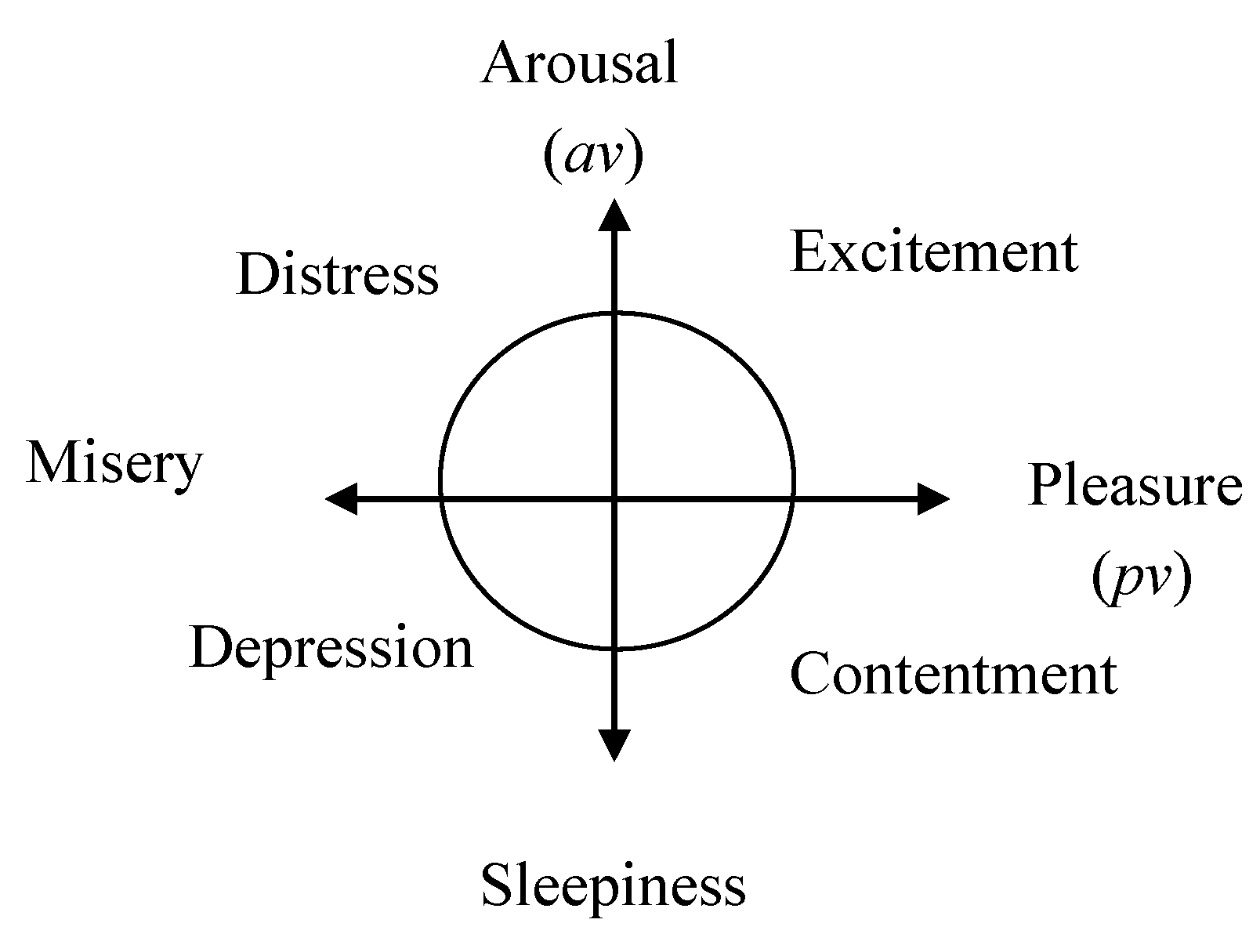
Russell’s circumplex model of affect [28] (See Figure 1) is simple and clear. It is given by a statistic method (principal-components analysis) to categorize human being’s affects using 343 subjects’ self-reports judgments. In the circumplex model, eight kinds of affective states including pleasure (0°), excitement (45°), arousal (90°), distress (135°), displeasure (180°), depression (225°), sleepiness (270°) and relaxation (315°) are located in a circular order. The interrelationships of these states are also represented by the arrangement, e.g., high values of arousal and pleasure result in a high value of excitement.

Figure 1. A circumplex model of affect proposed by Russell [27,28].

Figure 1. A circumplex model of affect proposed by Russell [27,28].

2.2. Emotion Function

In contrast with using the value function to decide an action/behavior of agents in conventional reinforcement learning methods [1,2,3,4,5,6,7,8,9,10,11,12,13,14,15,16,17,18,19,20,21,22], we propose using affective factors to invoke emotional response and reaction during the state transition process of agents in multi-agent systems (MASs). The reason for this proposal is according to the principle of interacting brain systems: the emotional brain and the thinking brain make decisions cooperatively [23,24]. Here, we use “Arousal” and “Pleasure” of Russell’s basic affects to construct “eliciting situation-oriented emotion” of agents. Moreover, the goal-directed problem that needs to be solved by RL is limited to pursuit problems or unknown environment explorations using local observable information.

Now, suppose an eliciting situation for an agent i, i ∈ {1,2,…,N} is e, e ∈ E ≡ {1,2,…,|E|}, and the corresponding emotion is Emo_i(e). When the agent perceives objects with high rewards (e.g., a goal) in the situation e, then Emo_i(e) = toPv_i(e) (see Equation (1)), where toPv_i(e) (see Equation (2)) is a mulptiplication of Arousal av_i(e) (see Equation (4)) and Pleasure Pv_i(e) (see Equation (5)). Meanwhile, if the agent finds other agents in the situation e, the emotion of the agent is totally effected by the emotion of other (perceived) agents Emo_i(a) = getPv_i(a) (see Equation (1)). Consequently, the emotion function of the agent i in the state a is given by Equations (1–5).

(1)

(2)

(3)

(4)

(5)

where d_goal(e) is Eclidean distance from the agent to a goal in enviroment exploration problem or a prey in pursuit problem if the goal is perceivable, and d_agent(e) denotes Eclidean distance between agent i and agent j if the agent j is perceivable in situlation e. Depth is the threshold value of perceivable depth of space for sensory stimuli of visual, auditory, or olfactory signals, ∆av, Pv, σ are positive parameters, e_i and e_i’ are the current and next eliciting situations respectively.

So the formulas designed above can be incorporated into the following inferences rules:

• Rule A: Pleasure pv_i(e) concerns with the distance between the agent i, i ∈ {1,2,…,N} and the goal (Equation (5)) if the situation e means that the goal is perceived .
• Rule B: Arousal av_i(e) increases when the eliciting situation is continued (Equation (4)).
• Rule C: Emotion state Emo_i(e) (Equations (1–3)) of agent i in the eliciting situation e is expressed by the multiplication of Pleasurepv_i(e) or pv_j(e) (Equation (5)) and Arousal av_i(e) or av_j(e) (Equation (4)).
• Rule D: Emotion state Emo_i(e) is constructed and changed by stimuli from objects and events: perceiving the goal or other agents dynamically (Equations (1–5)).

2.3. A Motivation Function

When the Q learning algorithm (QL) [1,21] of the convetional reinforcement learning (RL) is used to find the optimal solution of a Markov decision process (MDP) which describes the stochastic state transition of agents, a state-action value function Q_i(s,a) is calculated as follows:

(6)

where s ∈ R^N×|E| is a state oberved by the agent i, a ∈ R^|E| is an action selected by the agent according to the value of Q_i(s,a) (higher Q_i(s,a) serves higer probability of action a at the state a), s’, a’ are the next state and selectable action, and r is a scalar of reward from the environment, 0 < α < 1 is a learning rate, and 0 < γ < 1 a discount constant.

MDP, defined as the transition of states that only depends on the current state and the selected action [1], showed good convergence for the problems in MDP. However, in many real-world cases, Markov assumption is not satisfied. For example, when a learner observes its local environment or the state indirectly, different actions need to be selected for the optimal state transition. This case is called partially observable Markov decision process (POMDP) [1]. In MASs, an agent even needs to decide its optimal action according to the decision of other agents, so the problem of MASs belongs to non-Markov nature. To improve QL for POMDP and non-Markovian problems, approaches to change the environment to be MDP-like have been proposed, such as using belief state which uses the information of transition history [1,21], Monte-Carlo policy evaluation [35], and the different rewards of agents [36]. Furthermore, additional information such as the relationship between agents is also adopted into state-action value function in [18].

Here, agents learning of a MAS, we propose that it not only is decided by the value of observed state of environment, i.e., Equation (6), but also situation-oriented emotion of agent given by Equations (1–5). A motivation function of agent i to express state-emotion-action value is proposed as follows.

(7)

where 0 ≤ L ≤ 1.0 is a constant to adjust the balance of emotional response Emoi(e) and knowledge exploitation Q_i(s,a). Specifically, the action a, a ∈ A ≡ {1,2,…,|A|} denotes the action of agent i in each available situation e, |A| = |E| here.

2.4. Policy to Select an Action

As for the traditional QL, we use the soft-max seletion policy to decide an action according to the Bolzmann (Gibbs) distribution [1].

(8)

where p_i(a|s,Emo(e)) is the probability of selecting action a at state s and emotion Emo(e) of an eliciting situation e. T is a positive constant called “temperature” in the Blzmann distribution function. Higher T encourages the agent to select an available action more randomly. Here, we suggest using T ← T^Episode, 0 < T < 1, Episode = 1,2,…Episode to reduce T according to the increase of learning iteration (Episode) to obtain stable learning convergence.

2.5. Learning Algorithm

The improved QL algorithm then can be given as follows:

Step 1

Initialize Q_i(s,a) = 0; av_i = 0 for each agent i, i ∈ {1,2,…,N} and all obserable states s ∈ S and actions.

Step 2

Repeat following in each episode.

(1)

Return to the initial state.

(2)

Repeat the following until the final state.

• Observe the state s_i ∈ S of the environment, judge the situation e_i ∈ E if the goal or other agents appear in perceivable area, calculate emotion Emo_i(e) and motivation M_i(s, Emo_i(e), a) at the state s_i and situation e_i of each selectable actions, select an action a_i ∈ A according to the stochastic policy (Equation (8)).
• Execute the action a_i; observe a reward r and next state s_i’.
• Renew Q_i(s,a) according to Equation (6).

(3)

s_i ← s_i’

Step 3

Stop if episodes are repeated enough.

3. Computer Simulation

3.1. Definition of Pursuit Problem

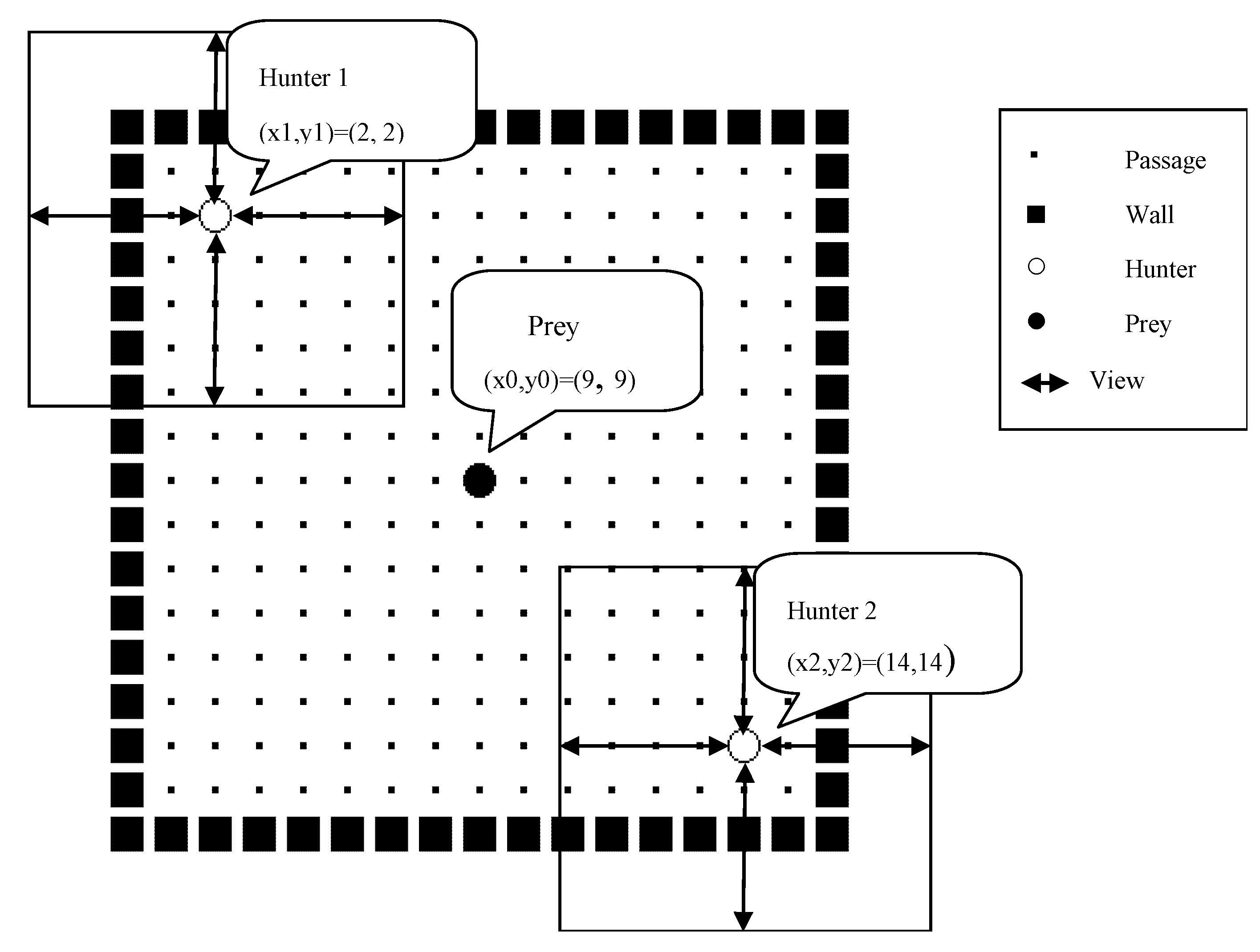
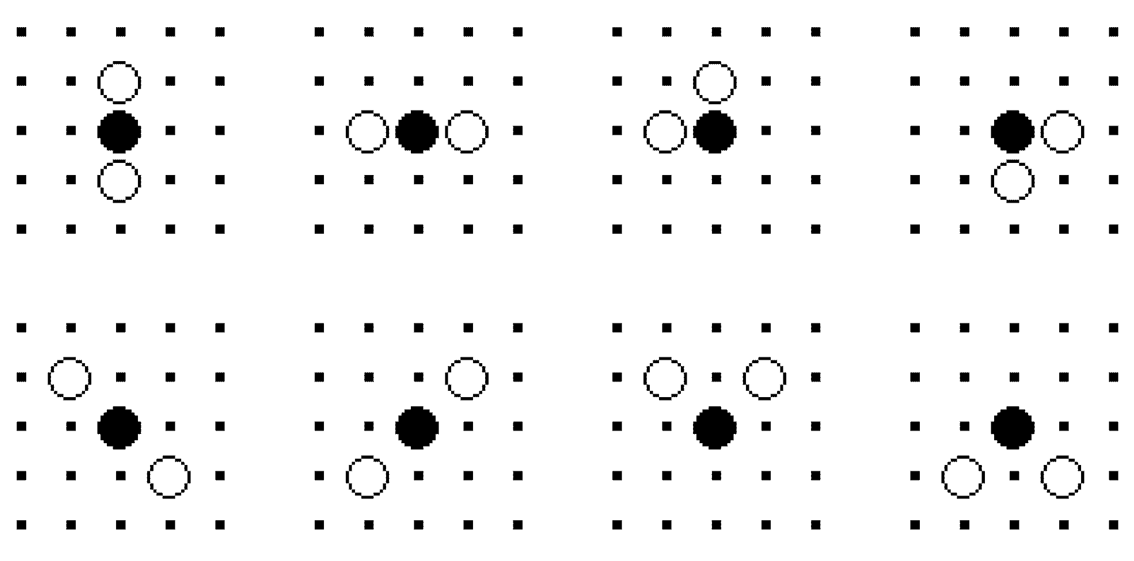
To confirm the effectiveness of the proposed method, computer simulations of pursuit problems were executed. In Figure 2, a case of 2-hunter-1-static-prey problem with its initial state of the exploration environment is shown. The size of the environment is 17 × 17 grids. Prey (ridstays at the position (9, 9) at all times, while two hunters (○) find and capture the prey from (2, 2) and (14, 14) respectively. The perceivable area of a hunter is a square field around the hunter as shown in Figure 2, and the depth limitation was set to be 4 grids in 4 directions. So, the global coordinate information was not used but local observable information, the environment belongs to PDMDP.

The pursuit problem, or hunting game, can be designed in various conditions [18], and for convenience, it is defined as a static or dynamic goal (prey) that needs to be captured by all plural agents (hunters) simultaneously as one of the final states, as shown in Figure 3.

A hunter, which is an autonomous agent, observes its local environment as a state in five dimensions: Wall or Passage in four directions (up, down, left, and right) and Prey information in one dimension. For the first four dimensions, there are three discrete values: near, far, and unperceivable. Prey dimension has five values: up, down, left, right, and unperceivable. So the number of states s_i observed by a hunter i is 4 × 3 × 5 = 60. The number of action is designed as |A| = 4 (up, down, left, right), and the number of state-action value function values Q_i(s,a) (Q table called in QL) is 60 × 4 = 240. Additionally, the emotional response Emo_i(e) to the eliciting situations, i.e., perception of prey or other agents, are also in four directions, as for the action: up, down, left, and right |E| = 4. So the number of motivation function M_i(s, Emo_i(e), a) is 240 × 4 = 960.

Figure 2. An environment for 2-hunter-1-static-prey problem.

Figure 2. An environment for 2-hunter-1-static-prey problem.

Figure 3. Available final states of a 2-hunter-1-static-prey problem. Prey (le final states of a 2-hunter-1-static-pr.

Figure 3. Available final states of a 2-hunter-1-static-prey problem. Prey (le final states of a 2-hunter-1-static-pr.

The learning performance of the Q learning method and the proposed method were compared for the pursuit problem in simulation. A part of the setting of simulations and parameters are listed in Table 1, Table 2. Special parameters used in the proposed method are listed in Table 3.

Table 1. Common conditions in the simulations.

Description	Symbol	Value
Episode limitation	Episode	200 times
Exploration limitation in one episode	step	10,000 steps
Size of the environment	X × Y	17 × 17 grids
Threshold (depth) of perceive field	Depth	4 grids
Number of hunter	i	2, 3, 4
Number of action/situation	a/e	4

Table 1. Common conditions in the simulations.

Description	Symbol	Value
Episode limitation	Episode	200 times
Exploration limitation in one episode	step	10,000 steps
Size of the environment	X × Y	17 × 17 grids
Threshold (depth) of perceive field	Depth	4 grids
Number of hunter	i	2, 3, 4
Number of action/situation	a/e	4

Table 2. Parameters used in the simulation of 2-hunter-1-static-prey problem.

Parameter	Symbol	Q learning	Proposed method
Learning rate	α	0.9	0.9
Damping constant	γ	0.9	0.9
Temperature (initial value)	T	0.99	0.994
Reward of prey captured by 2 hunters	r1	10.0	10.0
Reward of prey captured by 1 hunter	r2	1.0	1.0
Reward of one step movement	r3	−0.1	−0.1
Reward of wall crash	r4	−1.0	−1.0

Table 2. Parameters used in the simulation of 2-hunter-1-static-prey problem.

Parameter	Symbol	Q learning	Proposed method
Learning rate	α	0.9	0.9
Damping constant	γ	0.9	0.9
Temperature (initial value)	T	0.99	0.994
Reward of prey captured by 2 hunters	r1	10.0	10.0
Reward of prey captured by 1 hunter	r2	1.0	1.0
Reward of one step movement	r3	−0.1	−0.1
Reward of wall crash	r4	−1.0	−1.0

Table 3. Parameters of the proposed method used in the simulations.

Parameter	Symbol	Value
Coefficient of Emo	L	0.5
Coefficient of Pleasure	Pv	200.0
Initial value of Arousal	Av	1.0
Modification of Arousal	Δav	0.01
Constant of Gaussian function	σ	8.0

Table 3. Parameters of the proposed method used in the simulations.

Parameter	Symbol	Value
Coefficient of Emo	L	0.5
Coefficient of Pleasure	Pv	200.0
Initial value of Arousal	Av	1.0
Modification of Arousal	Δav	0.01
Constant of Gaussian function	σ	8.0

3.2. Results of Simulation with a Static Prey

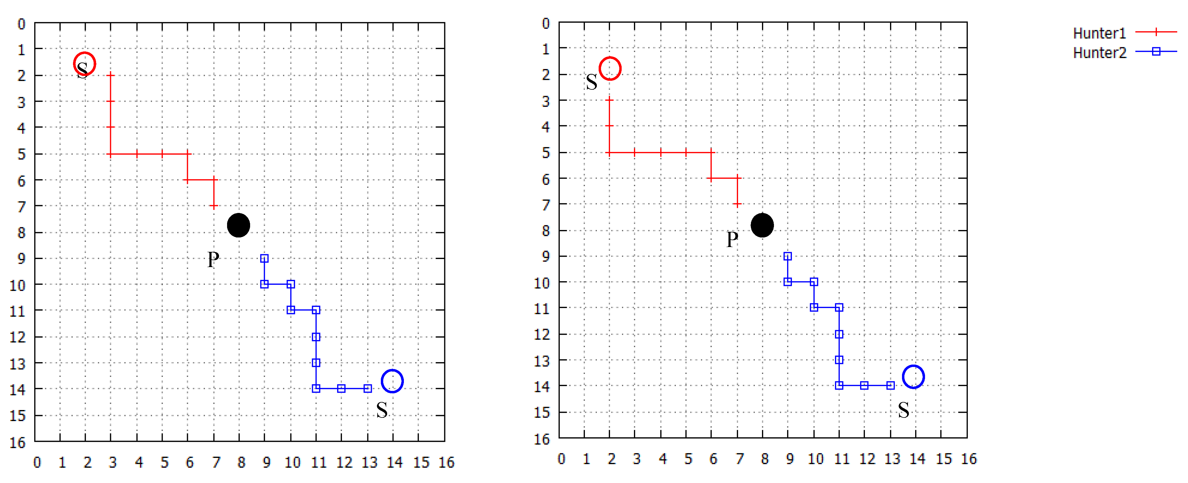
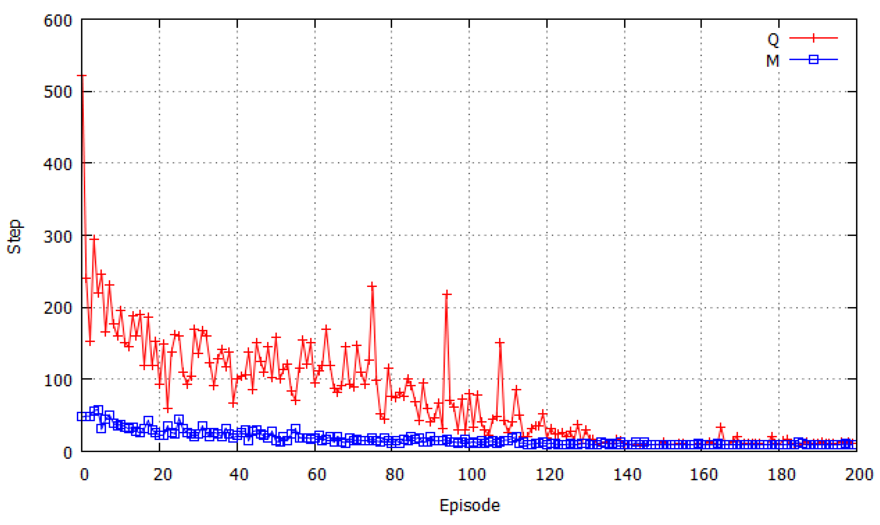
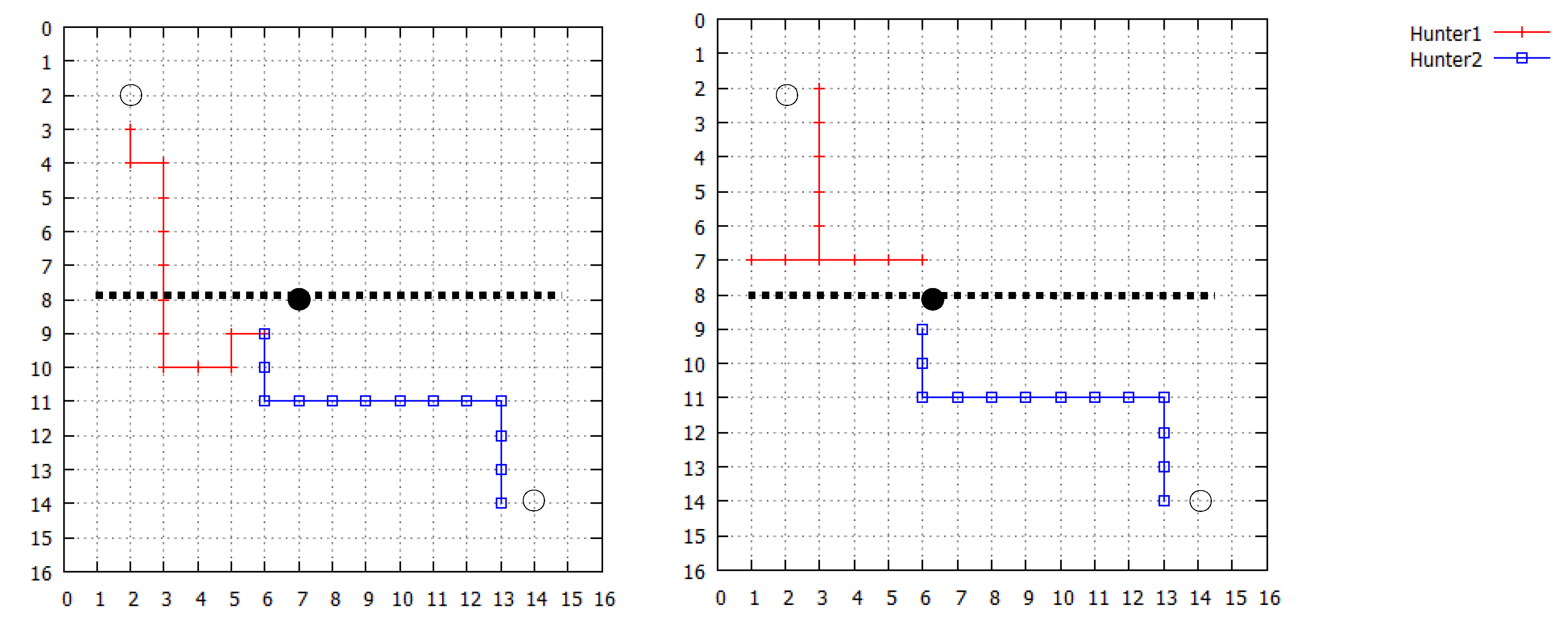
Both QL and the proposed method achieved the final states when learning process converged in the simulation. Figure 4 shows the different tracks of two hunters given by conventional QL (Figure 4(a)) and the proposed method (Figure 4(b)) where “S” denotes the start position of hunters, “○” denotes the start position of hunters and “●” is the position of the static prey. The convergence of the proposed method was faster and better than Q learning, as shown as in Figure 5 where “Q” indicates conventional QL results, and “M” is by the proposed motivation function used method.

Figure 4. Comparison of different tracks of two hunters captured a static prey. (a) Results of Q learning (QL); (b) Results of the proposed method.

Figure 4. Comparison of different tracks of two hunters captured a static prey. (a) Results of Q learning (QL); (b) Results of the proposed method.

Figure 5. Comparison of the change of exploration costs (the number of steps from start to final states) during learning process in 2-hunter-1-static-prey problem simulation (average of 10 simulations).

Figure 5. Comparison of the change of exploration costs (the number of steps from start to final states) during learning process in 2-hunter-1-static-prey problem simulation (average of 10 simulations).

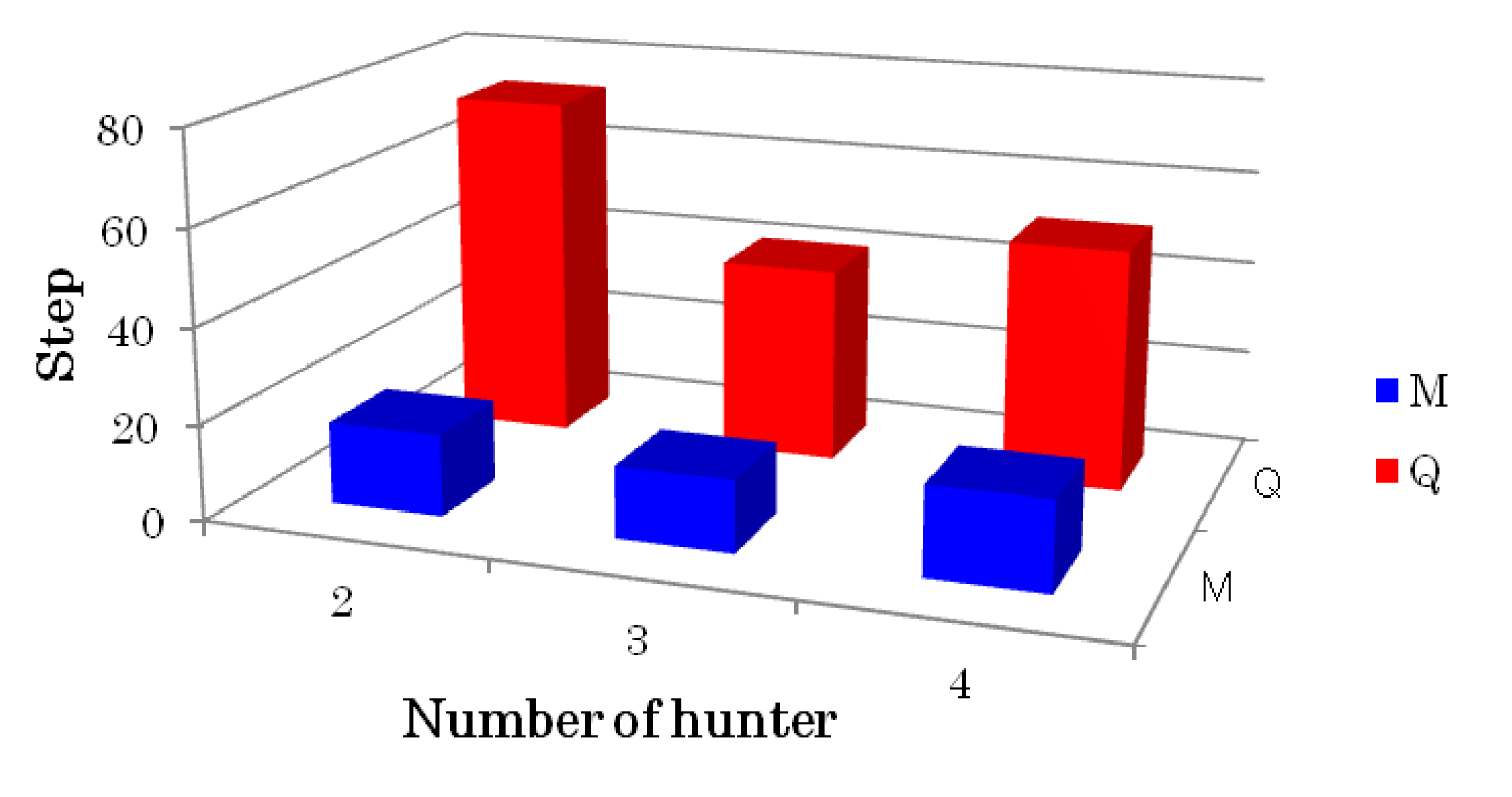
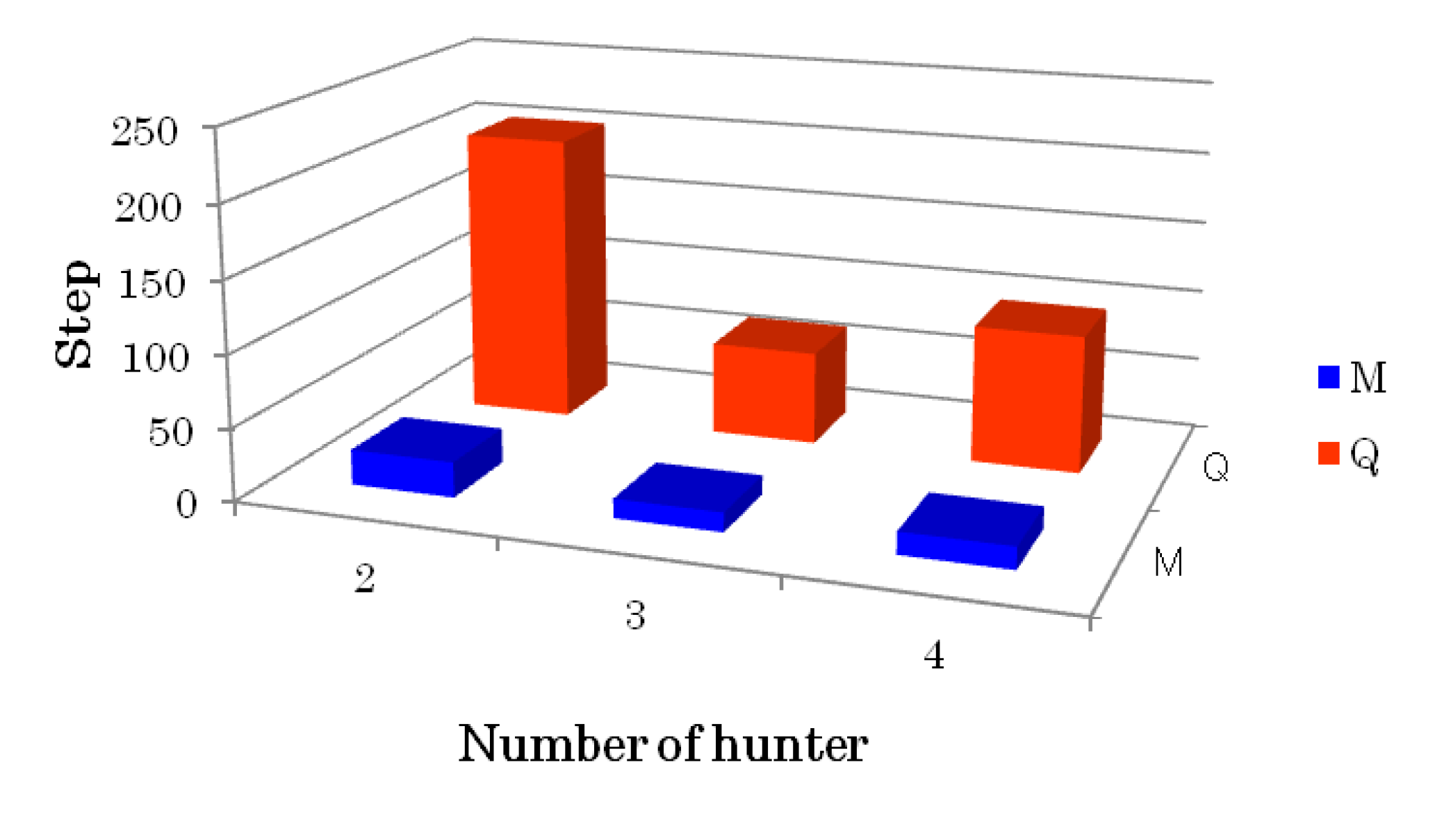
The average steps of one episode (from start to final states) during total learning process (200 episodes) given by 10 times simulations of the conventional QL and the proposed method were 72.9 and 17.1 as it shown in the first row of Table 4. Similar simulations using three and four hunters to find/capture a static prey were also performed and the learning performance of different methods was compared in Figure 6, Table 4. The proposed method was confirmed to be superior in terms of learning performance, i.e., it involves shorter steps to capture the prey in all simulations.

Table 4. Average exploration steps during learning in static prey problem simulations (200 episodes, 10 trials).

Number of hunter	Q learning	Proposed method
2	72.9	17.1
3	41.1	15.0
4	50.7	18.6

Table 4. Average exploration steps during learning in static prey problem simulations (200 episodes, 10 trials).

Number of hunter	Q learning	Proposed method
2	72.9	17.1
3	41.1	15.0
4	50.7	18.6

Figure 6. Comparison of average exploration steps during learning in static prey problem simulations (200 episodes, 10 trials).

Figure 6. Comparison of average exploration steps during learning in static prey problem simulations (200 episodes, 10 trials).

3.3. Results of Simulation with a Dynamic Prey

When a prey is not static, i.e., moves during the exploration process, the learning of hunters’ adaptive actions become more difficult. We designed a simulation of dynamic prey problem with a periodic movement process of the prey. The simulation was performed at the same start state, as shown in Figure 3. After the start state, the prey moved one step to the left before they arrived at the left wall. Then, it returned to the right direction until the right wall, and repeated the left-right movement periodically.

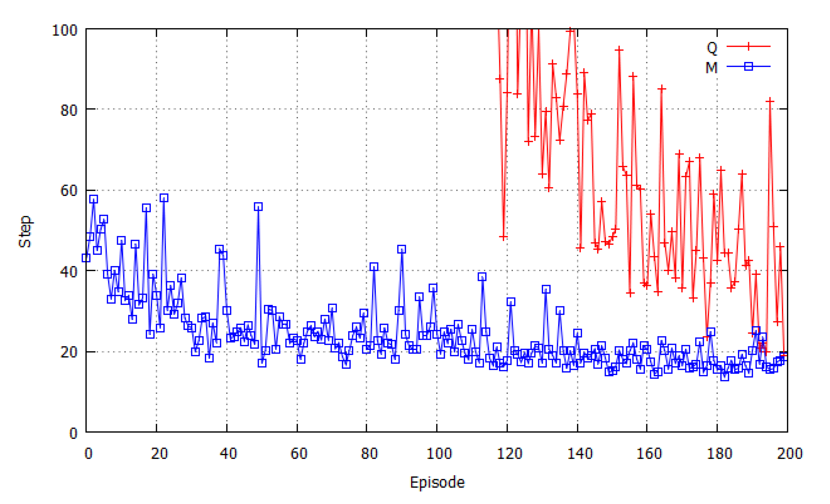
Table 5 gives the parameters used in a simulation of 2-hunters-1-dynamic-prey problem, and in Figure 7, the difference between the learning processes of different methods was shown, where “Q” means the result of conventional QL, and “M” depicts the change of exploration cost (steps) during learning (episode) using the proposed method.

Table 5. Parameters used in the simulation of 2-hunter-1-dynamic-prey problem.

Parameter	Symbol	QL	Proposed method
Learning rate	α	0.9	0.9
Damping constant	γ	0.9	0.9
Temperature (initial value)	T	0.99	0.99
Reward of prey captured by 2 hunters	r1	10.0	10.0
Reward of prey captured by 1 hunter	r2	1.0	1.0
Reward of one step movement	r3	−0.1	−0.1
Reward of wall crash	r4	−1.0	−1.0
Coefficient of Emo	L	-	0.5
Coefficient of Pleasure	Pv	-	10.0
Initial value of Arousal	Av	-	1.0
Modification of Arousal	Δav	-	0.1
Constant of Gaussian function	σ	-	8.0

Table 5. Parameters used in the simulation of 2-hunter-1-dynamic-prey problem.

Parameter	Symbol	QL	Proposed method
Learning rate	α	0.9	0.9
Damping constant	γ	0.9	0.9
Temperature (initial value)	T	0.99	0.99
Reward of prey captured by 2 hunters	r1	10.0	10.0
Reward of prey captured by 1 hunter	r2	1.0	1.0
Reward of one step movement	r3	−0.1	−0.1
Reward of wall crash	r4	−1.0	−1.0
Coefficient of Emo	L	-	0.5
Coefficient of Pleasure	Pv	-	10.0
Initial value of Arousal	Av	-	1.0
Modification of Arousal	Δav	-	0.1
Constant of Gaussian function	σ	-	8.0

Figure 7. Comparison of the change of exploration costs (the number of steps from start to final states) during learning process in 2-hunter-1-dynamic-prey problem simulation (average of 10 simulations).

Figure 7. Comparison of the change of exploration costs (the number of steps from start to final states) during learning process in 2-hunter-1-dynamic-prey problem simulation (average of 10 simulations).

In Figure 8, the trajectories of two hunters that pursued the dynamic prey were shown. In contrast to Figure 6, the trajectories of two hunters in Figure 8 were shown where they pursued the prey who moved to left or right directions (the broken lines). The trajectories were the solutions after 200 training (episodes) by different methods: Figure 8(a) shows conventional QL and Figure 8(b) the proposed method. The length of each trajectory was the same: 13 steps (the theoretical optimal solution is 11 steps).

Figure 8. Comparison of different tracks of two hunters capturing a dynamic prey. (a) Results of Q learning (QL); (b) Results of the proposed method.

Figure 8. Comparison of different tracks of two hunters capturing a dynamic prey. (a) Results of Q learning (QL); (b) Results of the proposed method.

Additionally, all average exploration steps during learning of different numbers of hunters for the dynamic prey problem are summarized in Table 6. As a result, the proposed method showed higher efficiency than conventional QL, and the effectiveness was more obvious than the case of static prey problems (Also see Figure 9).

Table 6. Average exploration steps during learning in dynamic prey problem simulations (200 episodes, 10 trials).

Number of hunter	Q learning (QL)	Proposed model (DEM)
2	202.7	24.4
3	65.1	13.3
4	96.0	15.3

Table 6. Average exploration steps during learning in dynamic prey problem simulations (200 episodes, 10 trials).

Number of hunter	Q learning (QL)	Proposed model (DEM)
2	202.7	24.4
3	65.1	13.3
4	96.0	15.3

Figure 9. Comparison of average exploration steps during learning in dynamic prey problem simulations (200 episodes, 10 trials).

Figure 9. Comparison of average exploration steps during learning in dynamic prey problem simulations (200 episodes, 10 trials).

4. Discussions

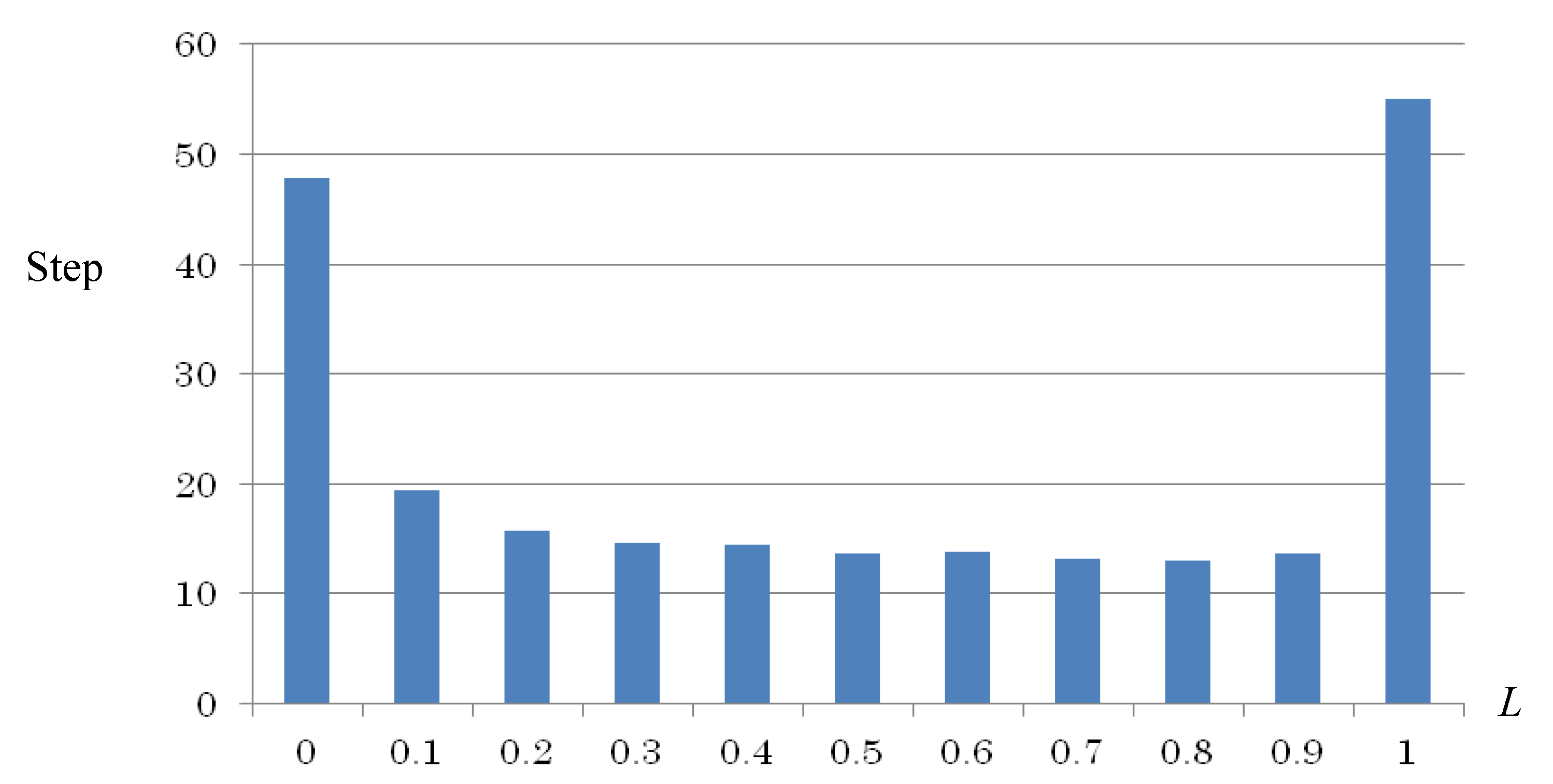
As the results of pursuit problem simulations, the proposed learning method which combined QL and affect factors enhanced the learning efficiency compared to the conventional QL. Parameters used in all methods were optimal values from experiments. For example, different values of balance coefficient L in Equation (7) may yield different learning performance. L = 0.5 was used either in static prey simulation as shown in Table 3, or in dynamic prey simulation as shown in Table 5 because the optimal value yielded the shortest path for each simulation. In Figure 10, a case of a simulation with three hunters and one dynamical prey was shown. The value of L increased from 0 to 1.0 by a difference of 0.1 in the horizontal axis, and the lowest value of the vertical axis shows the average length (steps) of the 10 simulations of the capture process to be 13.11 steps at L = 0.8, so L = 0.8 was used as the optimal parameter value in this case.

Figure 10. Comparison of the change of exploration costs (the number of steps from start to final states) by different Q-M balance coefficient L in Equation (7) during learning process in 3-hunter-1-dynamic-prey problem simulation (average of 10 simulations).

Figure 10. Comparison of the change of exploration costs (the number of steps from start to final states) by different Q-M balance coefficient L in Equation (7) during learning process in 3-hunter-1-dynamic-prey problem simulation (average of 10 simulations).

It is interesting to investigate how Arousal av and Pleasure pv values changed during the exploration and learning process in the simulation of pursuit problem. In Figure 11, the change of these affect factors in the 2-hunter-1-dynamic-prey simulation is depicted. In Figure 11(a), Arousal values of Hunters 1 and 2 changed together in the first three-step period, and then separated. This suggests that the state of the local environment observed by Hunter 1 changed more dramatically than the situation of Hunter 2, so Arousal av of Hunter 1 dropped according to the exploration steps. This is the result of Equation (4), the definition of Arousal av. In contrast, in Figure 11(b), Pleasure pv of Hunter 1 rose steeply to high values from step 2, corresponding to the dramatic change of the observed state: it might find and move to the prey straight ahead. From the 9th step, the Pleasure value of Hunter 2 also rose to high values for finding the prey or perceiving the high Pleasure value of Hunter 1.

From this analysis of the change of affect factors, it can be judged that the proposed method worked efficiently in the reinforcment learning process and it results in the improvement of learning performance of the MAS.

Figure 11. The change of Arousal av and Pleasure pv values of two hunters during the exploration in dynamic prey problem simulation. (a) The change of Arousal av; (b) The change of Pleasure pv.

Figure 11. The change of Arousal av and Pleasure pv values of two hunters during the exploration in dynamic prey problem simulation. (a) The change of Arousal av; (b) The change of Pleasure pv.

5. Conclusions and Future Works

To improve the learning performance of reinforcement learning for multi-agent systems (MASs), a novel Q-learning (QL) was proposed in this paper. The main idea of the improved QL is the adoption of affect factors of agents which constructed “situation-oriented emotion” and a motivation function which is the combination of conventional state-action value function and the emotion function.

Compared with the conventional QL, the effectiveness of the proposed method was confirmed by simulation results of pursuit problems with static and dynamic preys in the sense of learning costs and convergence properties.

The fundamental standpoint of this study to use affective and emotional factors in the learning process is in agreement with Greenberg [24]: “Emotion moves us and reason guides us”. Conventional QL may only pay attention to “reasoning” from “the thinking brain” [24], or basal ganglia [2]. Meanwhile, in the proposed method we also considered the role of “the emotion brain” [23], amygdala or limbic system [24].

Therefore, as expected, future works will identify functions such as the neuro-fuzzy networks [9,10,11,12,13,14], and more emotion functions such as fear, anger, etc. [31,32,37,38], and other behavior psychological views [39] may be added to the proposed method. All these function modules may contribute to a higher performance of autonomous agents and it is interesting to apply these agents to develop intelligent robots.

References

1. Sutton, R.S.; Barto, A.G. Reinforcement Learning: An Introduction; The MIT Press: Cambridge, MA, USA, 1998. [Google Scholar]
2. Doya, K. Metalearning and neuromodulation. Neural Netw. 2002, 15, 495–506. [Google Scholar] [CrossRef]
3. Asada, M.; Uchibe, E.; Hosoda, K. Cooperative behavior acquisition for mobile robots in dynamically changing real worlds via vision-based reinforcement learning and development. Artif. Intell. 1999, 110, 275–292. [Google Scholar] [CrossRef]
4. Kollar, T.; Roy, N. Trajectory optimization using reinforcement learning for map exploration. Int. J. Robot. Res. 2008, 27, 175–196. [Google Scholar] [CrossRef]
5. Jouffe, L. Fuzzy inference system learning by reinforcement learning. IEEE Trans. Syst. Man Cybern. B 1998, 28, 338–355. [Google Scholar] [CrossRef]
6. Obayashi, M.; Nakahara, N.; Kuremoto, T.; Kobayashi, K. A robust reinforcement learning using concept of slide mode control. Artif. Life Robot. 2009, 13, 526–530. [Google Scholar] [CrossRef]
7. Kuremoto, T.; Obayashi, M.; Yamamoto, A.; Kobayashi, K. Predicting Chaotic Time Series by Reinforcement Learning. In Proceedings of the 2nd International Conference on Computational Intelligence, Robotics, and Autonomous Systems, Singapore, 15–18 December 2003.
8. Kuremoto, T.; Obayashi, M.; Kobayashi, K. Nonlinear prediction by reinforcement learning. Lect. Note. Comput. Sci. 2005, 3644, 1085–1094. [Google Scholar]
9. Kuremoto, T.; Obayashi, M.; Kobayashi, K. Forecasting Time Series by SOFNN with Reinforcement Learning. In Proceedings of the 27th Annual International Symposium on Forecasting, Neural Forecasting Competition (NN3), New York, NY, USA, 24–27 June 2007.
10. Kuremoto, T.; Obayashi, M.; Kobayashi, K. Neural forecasting systems. In Reinforcement Learning, Theory and Applications; Weber, C., Elshaw, M., Mayer, N.M., Eds.; InTech: Vienna, Austria, 2008; pp. 1–20. [Google Scholar]
11. Kuremoto, T.; Obayashi, M.; Kobayashi, K.; Adachi, H.; Yoneda, K. A Reinforcement Learning System for Swarm Behaviors. In Proceedings of IEEE World Congress Computational Intelligence (WCCI/IJCNN 2008), Hong Kong, 1–6 June 2008; pp. 3710–3715.
12. Kuremoto, T.; Obayashi, M.; Kobayashi, K. Swarm behavior acquisition by a neuro-fuzzy system and reinforcement learning algorithm. Int. J. Intell. Comput. Cybern. 2009, 2, 724–744. [Google Scholar] [CrossRef]
13. Kuremoto, T.; Obayashi, M.; Kobayashi, K.; Adachi, H.; Yoneda, K. A neuro-fuzzy learning system for adaptive swarm behaviors dealing with continuous state space. Lect. Notes Comput. Sci. 2008, 5227, 675–683. [Google Scholar]
14. Kuremoto, T.; Obayashi, M.; Kobayashi, K. An improved internal model for swarm formation and adaptive swarm behavior acquisition. J. Circuit. Syst. Comput. 2009, 18, 1517–1531. [Google Scholar] [CrossRef]
15. Sycara, K.P. Multi-agent systems. Artif. Intell. Mag. 1998, 19, 79–92. [Google Scholar]
16. Mataric, J. Reinforcement learning in multi-robot domain. Auton. Robot. 1997, 4, 77–93. [Google Scholar] [CrossRef]
17. Makar, R.; Mahadevan, S. Hierarchical multi agent reinforcement learning. Adv. Neural Inf. Process. Syst. 2000, 12, 345–352. [Google Scholar]
18. Kobayashi, K.; Kurano, T.; Kuremoto, T.; Obayashi, M. Cooperative behavior acquisition using attention degree. Lect. Notes Comput. Sci. 2012, 7665, 537–544. [Google Scholar]
19. Barto, A.G.; Sutton, R.S.; Anderson, C.W. Neuron-like adaptive elements that can solve difficult learning control problems. IEEE Trans. Syst. Man. Cybern. 1983, 13, 834–846. [Google Scholar]
20. Sutton, R.S. Learning to predict by the method of temporal difference. Mach. Learn. 1988, 3, 9–44. [Google Scholar]
21. Watkins, C.; Dayan, P. Technical note: Q-learning. Mach. Learn. 1992, 8, 55–68. [Google Scholar]
22. Konda, V.R.; Tsitsiklis, J.N. Actor-critic algorithms. Adv. Neural Inf. Process. 2000, 12, 1008–1014. [Google Scholar]
23. LeDoux, J.E. The Emotional Brain: The Mysterious Underpinnings of Emotional Life; Siman & Schuster: New York, NY, USA, 1996. [Google Scholar]
24. Greenberg, L. Emotion and cognition in psychotherapy: The transforming power of affect. Can. Psychol. 2008, 49, 49–59. [Google Scholar] [CrossRef]
25. Sato, S.; Nozawa, A.; Ide, H. Characteristics of behavior of robots with emotion model. IEEJ Trans. Electron. Inf. Syst. 2004, 124, 1390–1395. [Google Scholar]
26. Kusano, T.; Nozawa, A.; Ide, H. Emergent of burden sharing of robots with emotion model (in Japanese). IEEJ Trans. Electron. Inf. Syst. 2005, 125, 1037–1042. [Google Scholar]
27. Larsen, R.J.; Diener, E. Promises and problems with the circumplex model of emotion. In Review of Personality and Social Psychology; Clark, M.S., Ed.; Sage: Newbury Park, CA, USA, 1992; Volume 13, pp. 25–59. [Google Scholar]
28. Russell, J.A. A circumplex model of affect. J. Personal. Soc. Psychol. 1980, 39, 1161–1178. [Google Scholar] [CrossRef]
29. Kuremoto, T.; Obayashi, M.; Kobayashi, K.; Feng, L.-B. Autonomic behaviors of swarm robots driven by emotion and curiosity. Lect. Notes Comput. Sci. 2010, 6630, 541–547. [Google Scholar]
30. Kuremoto, T.; Obayashi, M.; Kobayashi, K.; Feng, L.-B. An improved internal model of autonomous robot by a psychological approach. Cogn. Comput. 2011, 3, 501–509. [Google Scholar] [CrossRef]
31. Russell, J.A.; Feldman Barrett, L. Core affect, prototypical emotional episodes, and other things called emotion: Dissecting the elephant. J. Personal. Soc. Psychol. 1999, 76, 805–819. [Google Scholar] [CrossRef]
32. Russell, J.A. Core affect and the psychological construction of emotion. Psychol. Rev. 2003, 110, 145–172. [Google Scholar] [CrossRef]
33. Wundn, W. Outlines of Psychology; Wilhem Englemann: Leipzig, Germany, 1897. [Google Scholar]
34. Ortony, A.; Clore, G.; Collins, A. The Cognitive Structure of Emotions; Cambridge University Press: Cambridge, UK, 1988. [Google Scholar]
35. Jaakkola, T.; Singh, S.P.; Jordan, M.I. Reinforcement learning algorithm for partially observable Markov decision problems. Adv. Neural Inf. Process. Syst. 1994, 7, 345–352. [Google Scholar]
36. Agogino, A.K.; Tumer, K. Quicker Q-Learning in Multi-Agent Systems. Available online: http://archive.org/details/nasa_techdoc_20050182925 (accessed on 30 May 2013).
37. Augustine, A.A.; Hemenover, S.H.; Larsen, R.J.; Shulman, T.E. Composition and consistency of the desired affective state: The role of personality and motivation. Motiv. Emot. 2010, 34, 133–143. [Google Scholar] [CrossRef]
38. Watanabe, S.; Obayashi, M.; Kuremoto, T.; Kobayashi, K. A New Decision-Making System of an Agent Based on Emotional Models in Multi-Agent System. In Proceedings of the 18th International Symposium on Artificial Life and Robotics, Daejeon, Korea, 30 January–1 February 2013; pp. 452–455.
39. Aleksander, I. Designing conscious systems. Cogn. Comput. 2009, 1, 22–28. [Google Scholar] [CrossRef]