Backstepping Adaptive Sliding Mode Control for ROV Under Multi-Source Time-Varying Disturbances ^†

Abstract

To address the reduced motion control accuracy of underwater cleaning remotely operated vehicles (ROVs) caused by strongly coupled nonlinear dynamics and multisource time-varying disturbances, this study proposes a backstepping adaptive sliding mode control (B-ASMC) strategy. The proposed method combines the systematic design framework of backstepping control with the strong robustness of sliding mode control. An adaptive law is introduced to estimate the lumped system disturbance online and to compensate for it in real time, thereby avoiding dependence on an accurate disturbance observer or an exact system model. In addition, a hybrid thrust allocation strategy that integrates the pseudo-inverse method with the active-set method is developed to improve computational efficiency while suppressing thrust saturation. The global asymptotic stability of the closed-loop system is rigorously proved using Lyapunov stability theory. Simulations and tank experiments are conducted using a self-developed ROV. Simulation analyses under two representative operating conditions, namely depth holding and bow heading holding, show that B-ASMC achieves higher tracking accuracy, faster dynamic response, and stronger robustness than PID under time-varying disturbances. The tank experiments further verify that the proposed method exhibits control accuracy, disturbance rejection, and engineering applicability.

1. Introduction

During long-term marine operation, submerged surfaces of vessels, including hulls and propellers, are prone to extensive attachment of marine fouling organisms such as barnacles, calcareous tubeworms, and moss-like biofilms [1]. Regular cleaning of hulls and other wetted surfaces is therefore required. Underwater cleaning robots, or remotely operated vehicles (ROVs), offer clear advantages for such tasks in terms of safety, efficiency, and controllability [2]. However, ROV cleaning operations are affected by strong nonlinear and time-varying disturbances, including hydrodynamic damping, ocean current disturbances, umbilical cable drag, and reaction forces generated by cleaning devices. These disturbances can substantially degrade operational stability and positioning accuracy [3]. In addition, because ROVs exhibit strongly coupled nonlinear dynamics and their hydrodynamic parameters are difficult to identify accurately, high-precision motion control remains a challenging problem [4].

Considerable research efforts have been devoted to adaptive and robust control solutions for ROVs operating in complex marine settings. Various advanced strategies have been put forward, including adaptive regulation [5], robust approaches [6,7], sliding mode control, fuzzy logic schemes [8], and model predictive control [9,10]. Among these, sliding mode control stands out due to its well-known insensitivity to parametric uncertainties and external loads [11]. For example, Truong et al. devised a fixed-time terminal sliding mode controller that does not require any model information [12]. Huang and Yang introduced a dual-loop sliding mode architecture employing an arctangent switching function to mitigate chattering without sacrificing tracking fidelity [13]. Luo et al. constructed a double-closed-loop sliding mode regulator based on a nonlinear extended-state observer and a composite reaching law, which notably improved transient behavior and disturbance attenuation [14]. In another work, Deng and Tao integrated fractional-order calculus into the sliding mode framework, achieving accurate trajectory tracking even under input saturation [15]. Kim et al. merged sliding mode control with conventional time-delay compensation to boost position control in perturbed environments [16]. Chen et al. developed a model-free sliding mode controller inspired by neurodynamics, using a stretch-decay function derived from biological membrane potential regulation to suppress chattering and protect thrusters [17].

Several investigations have combined backstepping with sliding mode control for underwater vehicles. Backstepping offers a systematic nonlinear design procedure, ensuring global stability through recursive Lyapunov construction [18]. Raygosa-Barahona et al. proposed a model-free architecture that merges backstepping with second-order integral sliding mode, enabling robust trajectory tracking without an explicit ROV model [19]. Chen et al. put forward a backstepping integral sliding mode strategy that exploits the decomposition capability of backstepping alongside the rapid response and resilience of sliding mode; the integral action effectively cancels steady-state offsets induced by ocean currents [20]. Teji et al. developed a backstepping-based nonsingular terminal sliding mode control scheme that incorporates an adaptive law for estimating lumped uncertainties, guaranteeing finite-time convergence and disturbance robustness [21]. Liu et al. tackled uncertain disturbances from both internal and external sources by designing a cascade control system combining backstepping with a radial-basis-function neural network sliding mode controller, achieving coordinated kinematic and dynamic regulation [22].

Most current ROV control studies simplify ocean currents as either constant or periodic forcings [23]. While this simplification partially accounts for current effects, it fails to capture the genuine time-varying and stochastic characteristics of real ocean flows [24]. In response, the present work systematically explores the multi-dimensional impact of currents on ROV motion and aims to devise a controller that can flexibly accommodate diverse flow conditions. This effort furnishes technical support for enhancing ROV operational performance in complex marine environments.

(1) A hybrid thrust allocation strategy based on the pseudo-inverse method and the active-set method is designed. This strategy retains the fast solution speed of the pseudo-inverse method while effectively avoiding thrust saturation.

(2) An adaptive backstepping sliding mode control (B-ASMC) scheme is developed. By introducing an adaptive law to estimate and compensate for the lumped system disturbance online, the controller reduces its dependence on prior knowledge of the disturbance upper bound and on an accurate system model.

(3) Simulations and indoor tank experiments are conducted under two representative operating conditions, namely depth holding and bow heading holding, to verify the disturbance-rejection capability of B-ASMC under time-varying disturbances.

2. Mathematical Model of the ROV

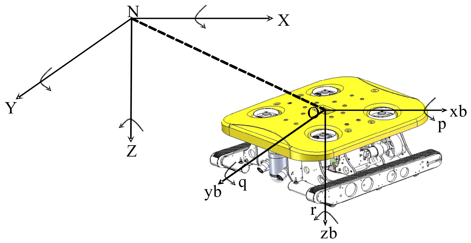
A ROV kinematic model was established to describe the ROV states, including position, attitude, linear and angular velocity, and linear and angular acceleration. Body-fixed and earth-fixed coordinate frames were defined. The $N-XYZ$ was regarded as an inertial coordinate frame, allowing the ROV state to be described in the moving frame and transformed between the body-fixed and earth-fixed frames through a rotation matrix. The coordinate-frame definitions are shown in Figure 1.

2.1. Kinematic Model

The ROV position vector in the earth-fixed frame is $P_n={[x,y,z]}^T$, and its attitude vector is ${\vartheta }_n={[\varphi ,\theta ,\psi ]}^T$. In the body-fixed frame, the linear velocity vector is $V_b={[u,v,w]}^T$, and the angular velocity vector is ${\omega }_b={[p,q,r]}^T$. The force vector expressed in the body-fixed frame is $f_b={[X,Y,Z]}^T$, and the corresponding moment vector is $m_b={[K,M,N]}^T$.

Accordingly, the 6-DOF motion of the underwater vehicle can be expressed as:

$$\eta =\left[\begin{array}{c}{P}_n\\ {\vartheta }_n\end{array}\right],V=\left[\begin{array}{c}{V}_b\\ {\omega }_b\end{array}\right],T=\left[\begin{array}{c}{f}_b\\ m_b\end{array}\right]$$

(1)

where $\eta$ is the pose vector in the fixed coordinate system, and $V$ and $T$ are the linear/angular velocity vector and the force/moment vector in the body-fixed coordinate system, respectively.

The linear velocity vector transformed to the fixed coordinate system is expressed as:

$${\dot{P}}_n=R_b^n(\vartheta )V_b$$

(2)

where $R_b^n(\vartheta ):=R_{z,\psi }{R}_{y,\theta }{R}_{x,\varphi }$ is the transformation matrix:

$$R_b^n=\left[\begin{array}{ccc}\cos \theta \cos \psi & -\cos \varphi \sin \psi +\sin \varphi \sin \theta \cos \psi & \sin \varphi \sin \psi +\cos \varphi \sin \theta \cos \psi \\ \cos \theta \sin \psi & \cos \varphi \cos \psi +\sin \varphi \sin \theta \sin \psi & -\sin \varphi \cos \psi +\cos \varphi \sin \theta \sin \psi \\ -\sin \theta & \sin \varphi \cos \theta & \cos \varphi \cos \theta \end{array}\right]$$

(3)

Therefore, the angular velocity transformation can be written as:

$$\begin{array}{c}{\dot{\vartheta }}_n=T(\vartheta ){\omega }_b\\ T(\vartheta )=\left[\begin{array}{ccc}1& \sin \varphi \tan \theta & \cos \varphi \tan \theta \\ 0& \cos \varphi & -\sin \varphi \\ 0& \sin \varphi /\cos \theta & \cos \varphi /\cos \theta \end{array}\right]\end{array}$$

(4)

Combining Equations (2) and (4) yields the 6-DOF kinematic equation of the ROV:

$$\dot{\eta }=J(\eta )V=\left[\begin{array}{cc}{R}_b^n(\vartheta )& 0_{3\times 3}\\ 0_{3\times 3}& T(\vartheta )\end{array}\right]\left[\begin{array}{c}{V}_b\\ {\omega }_b\end{array}\right]$$

(5)

2.2. Dynamic Model

The dynamic model is formulated using the vectorial modeling approach proposed by Fossen [3], which yields the rigid-body translational equation:

$$m[{\dot{V}}_b+{\dot{\omega }}_b\times r_g^b+{\omega }_b\times V_b+{\omega }_b\times ({\omega }_b\times r_g^b)]=f_b$$

(6)

where $r_g^b={[x_g,y_g,z_g]}^T$ is the position vector of the center of gravity in the body-fixed frame. Substituting the pose and velocity vectors yields the Newton–Euler equations, which can be expressed in the vector:

$$M_{RB}\dot{V}+C_{RB}(V)V=T_{RB}$$

(7)

where $M_{RB}$ is the rigid-body mass matrix, $C_{RB}(V)$ is the rigid-body Coriolis and centripetal matrix, and $T_{RB}$ denotes the forces and moments acting on the ROV, including restoring forces and moments, hydrodynamic forces, and environmental disturbance forces, as well as thruster forces. In the underwater environment, the gravity and buoyancy expressed in the body-fixed frame are given by:

$$f_g^b=R_b^n{(\vartheta )}^{-1}{f}_g^n,f_b^b=R_b^n{(\vartheta )}^{-1}{f}_b^n$$

(8)

The restoring force and moment can therefore be expressed as:

$$g(\eta )=-\left[\begin{array}{c}{f}_g^b+f_b^b\\ r_g^b\times f_g^b+r_b^b\times f_b^b\end{array}\right]$$

(9)

where $r_g^b$ and $r_b^b$ denote the positions of the center of gravity and the center of buoyancy in the body-fixed frame, respectively. Because the ROV hydrodynamic parameters are difficult to measure accurately, the ROV hydrodynamic terms are decomposed into inertial and viscous components for modeling:

$$T_H=M_A\dot{V}+C_A(V)V+D_N(V)V+D_L(V)V$$

(10)

where $M_A$ is the added mass matrix, $C_A$ is the added Coriolis matrix, $D_N$ is the nonlinear damping matrix, and $D_L$ is the linear damping matrix. Inertial hydrodynamic forces arise when an object accelerates or decelerates in an ideal fluid, forcing the surrounding fluid to move accordingly and thereby generating a reaction force on the object. The relationship between the inertial hydrodynamic force and the object acceleration is expressed as:

$$F_M=-{\displaystyle \sum _{i=1}^6{\lambda }_{ij}{\dot{V}}_i},(i,j=1,\mathrm{2...6})$$

(11)

where ${\lambda }_{ij}$ is the added-mass coefficient. Similar to the rigid-body dynamic model, added mass also generates an added Coriolis and centripetal matrix:

$$C_A(V)=\left[\begin{array}{cc}{0}_{3\times 3}& -S(A_{11}{v}_1+A_{12}{v}_2)\\ -S(A_{11}{v}_1+A_{12}{v}_2)& -S(A_{21}{v}_1+A_{22}{v}_2)\end{array}\right]$$

(12)

The hydrodynamic damping term is expanded into first-order linear and second-order nonlinear polynomial terms:

$$F_D={\displaystyle \sum _{i=1}^6(F_V{}_{i}V_i+F_{V_i{V}_j}{V}_i{V}_j)},(i,j=1,\mathrm{2...6})$$

(13)

where ${F_V}_i$ is the first-order hydrodynamic damping coefficient, and $F_{V_i{V}_j}$ is the second-order hydrodynamic damping coefficient. The viscous hydrodynamic force can be simplified as:

$$F_D=-D(V)V=-[D_N(V)+D_L(V)]V$$

(14)

During underwater navigation, wind- and wave-induced disturbances are relatively small; the ROV is mainly affected by current-induced environmental disturbances [25].

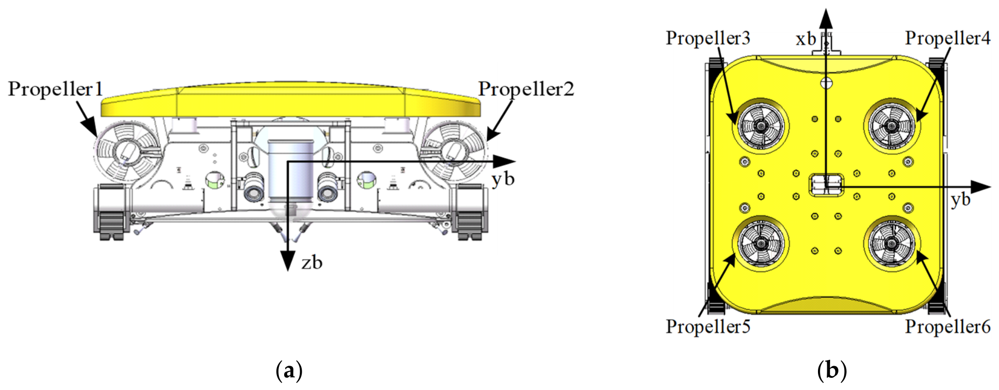
The ROV is equipped with four vertical thrusters and two horizontal thrusters, enabling 6-DOF motion. The thruster configuration is shown in Figure 2. The 6-DOF force and moment generated in the body-fixed frame can be expressed as:

$${\tau }_i=\left[\begin{array}{c}{F}_i\\ P_i\times F_i\end{array}\right]$$

(15)

where $F_i$ is the thrust vector, $P_i$ is the installation-position vector. Because the thrust outputs of the thrusters are coupled, the 6-DOF output force can be obtained as:

$$T=Bu$$

(16)

where $T$ denotes the resultant force and moment jointly produced by the six thrusters; $u$ denotes the thrust vector of the six thrusters; and $B$ denotes the spatial configuration matrix of the thrusters:

$$B=\left[\begin{array}{cccccc}1& 1& 0& 0& 0& 0\\ 0& 0& 0& 0& 0& 0\\ 0& 0& 1& 1& 1& 1\\ 0& 0& -0.254& 0.254& -0.254& 0.254\\ 0& 0& -0.28& -0.28& 0.28& 0.28\\ -0.43& 0.43& 0& 0& 0& 0\end{array}\right]$$

(17)

Finally, rearranging the dynamic Equation (6) gives:

$$M\dot{V}+C(V)V+D(V)V+g(\eta )=T+W$$

(18)

where $M=M_{RB}+M_A$ is the mass matrix, $C(V)=C_{RB}(V)+C_A(V)$ is the Coriolis and centripetal matrix, $D(V)=D_N(V)+D_L(V)$ is the hydrodynamic damping matrix, $g(\eta )$ is the restoring force and moment, and $W$ is the disturbance force and moment.

Through the SolidWorks 2023 Simulation module, partial design parameters of the underwater vehicle are obtained as follows: $m=160$ kg, the center of gravity $r_g^b={\left[0,0,0\right]}^T$ coincides with the origin of the body-fixed coordinate system, and the center of buoyancy $r_b^b={\left[0,0,-0.02\right]}^T$. Since the ROV operates at relatively low speeds, the off-diagonal elements of the inertia matrix have negligible effects on the motion. Accordingly, the rigid-body mass matrix $M_{RB}=diag\left\{160,160,160,15.2,20.5,18.7\right\}$.

To simplify the computation while maintaining model fidelity, appropriate simplifications are made by neglecting certain off-diagonal elements of the added mass matrix:

$$M_A=-\left[\begin{array}{cccccc}154.778& 0& 0& 0& 0& 0\\ 0& 160.339& 0& 2& 0& 1.5\\ 0& 0& 197.31& 0& 2.3& 0\\ 0& 2& 0& 2.11& 0& 2.1\\ 0& 0& 2.3& 0& 14.468& 0\\ 0& 1.5& 0& 2.1& 0& 12.848\end{array}\right]$$

(19)

By neglecting the off-diagonal elements of the viscous hydrodynamic damping matrix, we obtain:

$$\begin{array}{c}{D}_L(V)=-diag\left\{\begin{array}{cc}\begin{array}{ccc}0.49& 0.2& 0.13\end{array}& \begin{array}{ccc}0.26& 0.2& 0.2\end{array}\end{array}\right\}\\ D_N(V)=-diag\left\{\begin{array}{cc}\begin{array}{ccc}253& 310& 323\end{array}& \begin{array}{ccc}23& 39& 30\end{array}\end{array}\right\}\end{array}$$

(20)

2.3. Thrust Allocation Strategy

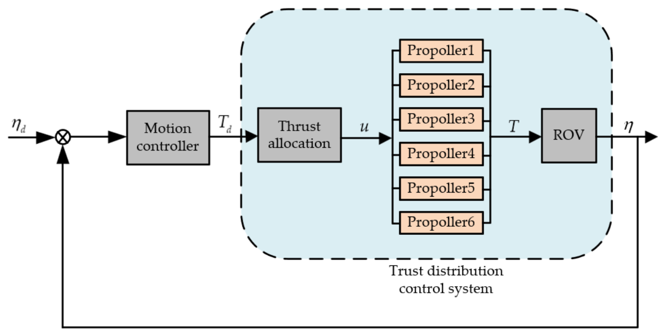
Quadratic optimization theory is introduced in this study. When the output obtained using the pseudo-inverse method reaches the performance limits of the thrusters, an optimization problem is solved iteratively. This strategy maintains a high solution speed while effectively avoiding thrust saturation [26]. The Schematic of the thrust allocation system is shown in Figure 3.

According to Equation (16), the relationship between propeller efficiency and thruster force can be fitted by the following quadratic function:

$${\tilde{\eta }}_i=a_1{u}_i{}^2+a_2{u}_i+a_3$$

(21)

where $a_1$, $a_2$ and $a_3$ are constants. An optimization problem is then established with the objective of maximizing thruster output efficiency:

$$\max J={\displaystyle \sum _{i=1}^n{\tilde{\eta }}_i}=a_1{u}^{T}u+a_2{u}_m+8a_3$$

(22)

When $a_1<0$, the desired thruster output is specified, and the linear term can therefore be approximated as a constant. The objective function is simplified as:

$$\begin{array}{l}\min J=u^T\tilde{W}u\\ s.t.\hspace{0.5em}T-Bu=0\end{array}$$

(23)

where $\tilde{W}={\tilde{W}}_1{\tilde{W}}_2\dots {\tilde{W}}_m$ is the weight matrix of the propulsion system and is a diagonal positive-definite matrix. When the system configuration becomes singular, the pseudo-inverse method may yield a rank-deficient control law and fail to obtain an effective solution. A slack factor λ is therefore introduced to relax the constraints appropriately within the allowable input–output error range. By adjusting the value of $\lambda$, the feasible solution region of the optimization problem can be regulated. A hybrid optimization objective that minimizes allocation error while maximizing efficiency is then formulated as:

$$\begin{array}{l}\min J=\lambda {‖T-T_d‖}_2^2+u^T\tilde{W}u\\ s.t.\hspace{0.5em}\hspace{0.5em}\hspace{0.5em}T-Bu=0\end{array}$$

(24)

where $T_d$ is the desired six-degree-of-freedom force/moment vector, and $\lambda$ is the slack factor. The pseudo-inverse thrust allocation control law is obtained as:

$$u={\left(B^T\lambda B+\tilde{W}\right)}^{-1}{B}^T\lambda T_d$$

(25)

Substituting the equality constraint in Equation (24) into the objective function and expanding it gives:

$$\begin{array}{c}\min J={\displaystyle \frac{1}{2}}{u}^T\left[2\left(B^T\lambda B+\tilde{W}\right)\right]u-2\left(T_d{}^T\lambda B\right)u+T_d{}^T\lambda T_d\\ s.t.\hspace{0.5em}\hspace{0.5em}\hspace{0.5em}\hspace{0.5em}{u}_{\min }\le u\le u_{\max }\end{array}$$

(26)

Equation (26) is a constrained quadratic programming problem with a quadratic objective function and linear constraints. It can be written in the following standard form:

$$\begin{array}{c}\min J={\displaystyle \frac{1}{2}}{u}^{T}Gu+c^{T}u\\ s.t.\hspace{0.5em}\begin{array}{c}{a}_{i}u-b_i\ge 0,\end{array}i\in I\end{array}$$

(27)

where

$$\begin{array}{l}G=2\left(B^T\lambda B+\tilde{W}\right),\\ c^T=-2\left(T_d{}^T\lambda B\right)\\ a_i=\left[\begin{array}{c}{E}_{6\times 6}\\ -E_{6\times 6}\end{array}\right],b_i=\left[\begin{array}{c}{u}_{\min }^{1\times 6}\\ u_{\max }^{1\times 6}\end{array}\right]\end{array}$$

(28)

It is only necessary to select an appropriate slack factor $\lambda$ such that $G$ is positive definite. Because the covariance matrix $G$ can be shown to be positive semidefinite, the resulting problem is a convex quadratic programming problem and can be solved by the active-set method [27]. The advantage of the active-set method lies in its ability to take a known feasible solution as the starting point at each iteration and to move along the constraint boundaries until the optimal solution of the problem is reached. First, from Equation (27), an equality-constrained quadratic programming problem can be derived:

$$J(u)=J(u_k+p)={\displaystyle \frac{1}{2}}{p}^{T}Gp+g_k{}^{T}p+{\displaystyle \frac{1}{2}}{u}_k{}^{T}G{u}_k+u_k{}^{T}c$$

(29)

where $u_k$ denotes the current feasible iterate, and p denotes the forward direction. At the $k$th iteration, the equality-constrained QP subproblem to be solved is:

$$\begin{array}{c}\min J={\displaystyle \frac{1}{2}}{p}^{T}Gp+g_k{}^{T}p\\ s.t.\hspace{0.5em}\begin{array}{c}{a}_i{}^{T}p=0,\end{array}i={\delta }_k\end{array}$$

(30)

where ${\delta }_k$ is the set of satisfied equality constraints, and the optimal solution of the above equality-constrained QP problem is denoted by $P_k$. The active-set iterations are as shown in

Table 1. The active-set iterations.

Step	Action
1	Given an initial feasible solution $u_k$, determine the corresponding working set ${\delta }_k$, and set $k$ = 1.
2	Solve the equality-constrained subproblem in Equation (25). If the resulting optimal solution $P_k$ is zero, proceed to Step 5; otherwise, proceed to Step 3.
3	When $P_k\ne 0$, $a_k$ is obtained from Equation (26) and $u_{k+1}=u_k+a_k{p}_k$
4	If $a_k<1$, let ${\delta }_{k+1}={\delta }_k\cup \left\{i\right\}$ and return to Step 2. If $a_k=1$, then we obtain the working set ${\delta }_{k+1}={\delta }_k$, let $u_{k+1}=u_k+p_k$ and return to Step 2.
5	Use the Lagrange multiplier method to obtain the multipliers of the equality-constrained subproblem ${\lambda }_k$ associated with the current working set. If ${\lambda }_k{}^j\ge 0$, the optimal solution has been obtained, and the iteration terminates; otherwise, remove the corresponding constraint and return to Step 2

.

Accordingly, this study proposes a hybrid thrust allocation strategy that combines the improved pseudo-inverse method with the active-set method. The strategy retains the rapid solution capability of the pseudo-inverse method while effectively avoiding thrust saturation.

3. Controller Design

3.1. B-ASMC Design

The ROV dynamic model can be transformed into a general second-order nonlinear equation. Because the ROV operates at low speed during attitude regulation, the Coriolis term can be neglected; hence, Equation (18) can be simplified as:

$$M\left[\dot{J}{(\eta )}^{-1}\dot{\eta }+J{(\eta )}^{-1}\ddot{\eta }\right]+D(\eta )J{(\eta )}^{-1}\dot{\eta }+g(\eta )=u+\mathrm{\Delta }d$$

(31)

The tracking error of the attitude angle is defined as:

$$z_1=x_1-x_d$$

(32)

where $x_d$ is the desired input attitude angle. Differentiating the above equation gives:

$${\dot{z}}_1={\dot{x}}_1-{\dot{x}}_d=x_2-{\dot{x}}_d$$

(33)

The state equation of the ROV can be written as:

$$\left\{\begin{array}{c}{\dot{x}}_1=x_2\\ {\dot{x}}_2=\ddot{\eta }\end{array}\right.$$

(34)

where the state variable $x_1=\eta$ is selected. From the dynamic model Equation (21), we obtain:

$$\ddot{\eta }=(-J(\eta )\dot{J}{(\eta )}^{-1}-J(\eta )M^{-1}D(\eta )J{(\eta )}^{-1})x_2+J(\eta )M^{-1}u+J(\eta )M^{-1}\mathrm{\Delta }d-J(\eta )M^{-1}g(\eta )$$

(35)

which can be simplified as:

$$\ddot{\eta }=A{x}_2+g(\eta ,t)u+d(\eta ,t)+f(\eta ,t)$$

(36)

where $f$ and $g$ are general nonlinear functions, $d$ includes external disturbances, and $\left|d\left(\eta ,t\right)\right|\le D$. A conventional backstepping controller requires accurate error measurements and cannot guarantee sufficient robustness. Therefore, a sliding mode term is introduced to suppress unknown disturbances. The ROV state equation can then be written in disturbance-inclusive form:

$$\left\{\begin{array}{c}{\dot{x}}_1=x_2=\dot{\eta }\\ {\dot{x}}_2=A{x}_2+f(\eta ,t)+g(\eta ,t)u+F\end{array}\right.$$

(37)

where $F$ is the lumped uncertainty of the system, and we assume that $F$ is bounded, i.e., $\left|F\right|\le \overline{F}$. Define the Lyapunov function as:

$$V_1={\displaystyle \frac{1}{2}}{z}_1^2$$

(38)

Define $z_2$ as the virtual control variable. According to the Lyapunov stability criterion, one may choose:

$$x_2=-c_1{z}_1+{\dot{x}}_d+z_2$$

(39)

where $c_1$ is a constant satisfying $c_1>0$. Substituting the above expression into the Lyapunov function gives:

$${\dot{V}}_1=-c_1{z}_1{}^2+z_1{z}_2$$

(40)

It can be seen that if $z_2=0$, then $\dot{V}\le 0$ can be proven, and the system is ultimately asymptotically stable. Combining this result with sliding mode control, the switching function is defined as:

$$\sigma =k_1{z}_1+z_2=(k_1+c_1)z_1+{\dot{z}}_1$$

(41)

where $k_1>0$. It follows that $k_1+c_1>0$; if $\sigma =0$, then $z_1=0,z_2=0$ and ${\dot{V}}_1\le 0$.

Because the upper bound of the ROV lumped uncertainty $\overline{F}$ must be known, the lumped disturbance needs to be estimated to determine the controller parameters. Adaptive design is adopted to estimate the uncertainty accurately. The corresponding Lyapunov function is:

$$V_2=V_1+{\displaystyle \frac{1}{2}}{\sigma }^2+{\displaystyle \frac{1}{2\gamma }}{\tilde{F}}^2$$

(42)

where $\tilde{F}=F-\widehat{F}$ is the estimation error of $F$; $\widehat{F}$ is the estimate of $F$; and $\gamma$ is a positive constant. Thus:

$${\dot{V}}_2={\dot{V}}_1+\sigma \left[k_1(z_2-c_1{z}_1)+A{x}_2-{\ddot{x}}_d+F+f+c_1{\dot{z}}_1+gu\right]-{\displaystyle \frac{1}{\gamma }}\tilde{F}\dot{\widehat{F}}$$

(43)

Substituting the estimated value and the estimation error for the actual uncertainty $F$ gives:

$${\dot{V}}_2={\dot{V}}_1+\sigma \left[k_1(z_2-c_1{z}_1)+A{x}_2-{\ddot{x}}_d+\widehat{F}+f+c_1{\dot{z}}_1+gu\right]-{\displaystyle \frac{1}{\gamma }}\tilde{F}(\dot{\widehat{F}}-\gamma \sigma )$$

(44)

Accordingly, the B-ASMC control law is designed as:

$$u={\displaystyle \frac{1}{g}}\left[-k_1(z_2-c_1{z}_1)-A{x}_2+{\ddot{x}}_d-\widehat{F}-f-c_1{\dot{z}}_1-B_1\right]$$

(45)

where $B_1=h(\sigma +\beta \mathrm{sgn}(\sigma ))$ and $h$, $\beta$ are positive constants. The adaptive law is designed as $\dot{\widehat{F}}=-\gamma \sigma$.

3.2. Stability Proof

Substituting the control law Equation (45) into the Lyapunov function Equation (37) yields:

$$\begin{array}{ll}{\dot{V}}_2& =z_1{z}_2-c_1{z}_1{}^2-h{\sigma }^2-h\beta \left|\sigma \right|-\widehat{F}\\ & \le z_1{z}_2-c_1{z}_1{}^2-h{\sigma }^2-h\beta \left|\sigma \right|\end{array}$$

(46)

This expression can be written in matrix form. Let:

$$Q=\left[\begin{array}{cc}{c}_1+h{k}_1^2& h{k}_1-{\displaystyle \frac{1}{2}}\\ h{k}_1-{\displaystyle \frac{1}{2}}& h\end{array}\right]$$

(47)

Then, we obtain:

$$z^{T}Qz=c_1{z}_1{}^2-z_1{z}_2+h{\sigma }^2$$

(48)

If matrix $Q$ is positive definite, then:

$${\dot{V}}_2\le -z^{T}Qz-h\beta \left|\sigma \right|\le 0$$

(49)

By designing the determinant of matrix $Q$ as:

$$\left|Q\right|=h(c_1+k_1)-{\displaystyle \frac{1}{4}}$$

(50)

Therefore, by selecting appropriate $h$, $c_1$ and $k_1$ values, $Q$ can be guaranteed to be positive definite.

4. Simulation Results

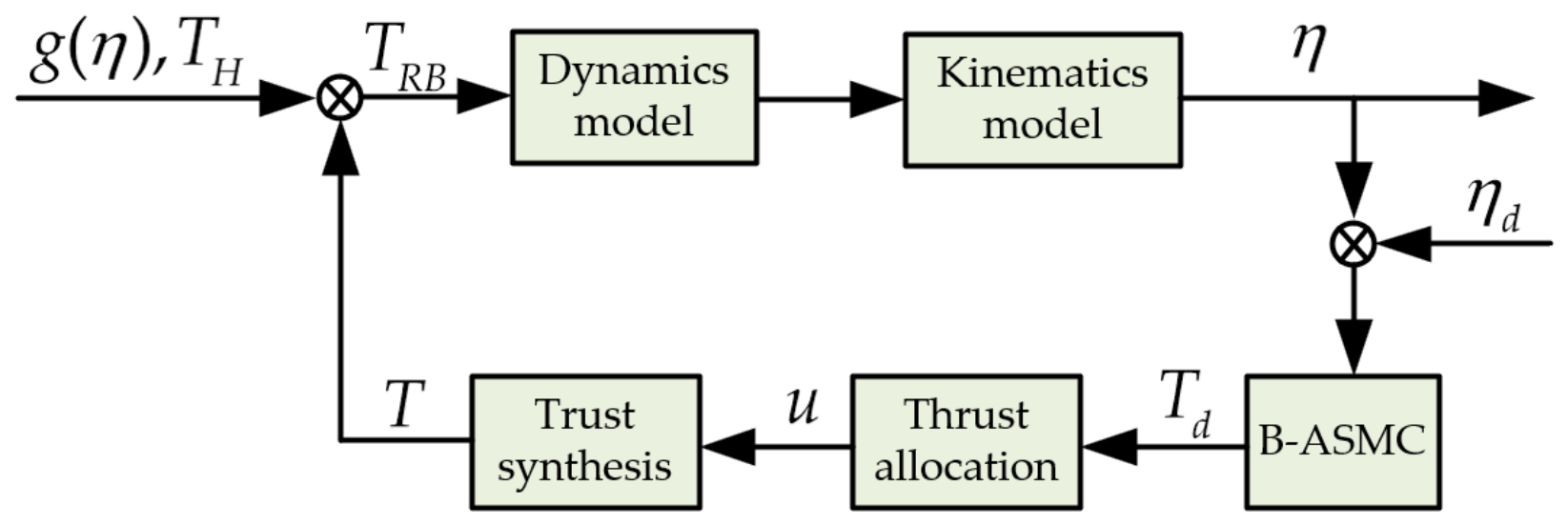
The preceding sections established the kinematic and dynamic models of the underwater cleaning robot, designed the hybrid thrust allocation strategy, and the B-ASMC. In this section, simulation analysis is performed on a ROV simulation model built in Simulink. The simulation model consists of four parts: the ROV dynamics solver, the motion controller, the thruster thrust allocation module, and the target control parameters. The overall simulation scheme is shown in Figure 4.

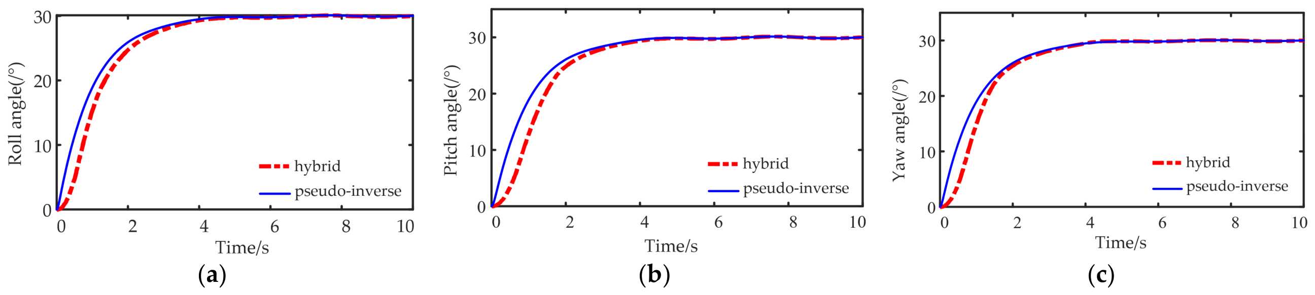
First, a comparative simulation analysis is conducted to evaluate the thrust allocation performance of the pseudo-inverse method and the hybrid thrust allocation strategy that combines our improved pseudo-inverse method with an active-set method with attitude control. The ROV is commanded to maintain its initial position and attitude, while the target roll, pitch, and yaw angles are simultaneously set to 30° in two separate cases. A specified disturbance signal is applied to the system for simulation analysis.

In addition, ROV depth-holding and bow heading-holding simulations are conducted under two operating conditions, namely without and with disturbances. Each condition includes constant and time-varying reference signals. The same controller parameters are used for the depth-holding and bow heading-holding cases. PID is characterized by a simple structure, clear physical concepts, and strong robustness, and has been widely applied in underwater vehicle control. When employing PID, an accurate mathematical model of the controlled plant is not required; only parameter tuning is needed. The control law of the PID is discretized and rewritten in sampled form as follows:

$$\begin{array}{l}u(k)=K_P\left\{e(k)+{\displaystyle \frac{T}{T_I}}{\displaystyle \sum _{j=0}^{k}e(j)}+{\displaystyle \frac{T_D}{T}}\left[e(k)-e(k-1)\right]\right\}\\ =K_{P}e(k)+K_I{\displaystyle \sum _{j=0}^{k}e(j)}+K_D\left[e(k)-e(k-1)\right]\end{array}$$

(51)

where $K_P$, $K_I$, $K_D$ are the proportional, integral, and differential coefficients, respectively; $T_I$ is the integral constant; $T_D$ is the differential constant; $e$ is the error; $T$ is the sampling period; and $k$ is the sampling sequence number.

From the control law, it is evident that the integral term requires cumulative summation of all previous error states, which implies that the state variables at every sampling instant must be stored. As the number of sampling instants increases, the computational burden on the processor grows substantially. To alleviate this issue, the incremental form of the PID algorithm is adopted, yielding the following:

$$\mathrm{\Delta }u(k)=u(k)-u(k-1)=K_P\mathrm{\Delta }e(k)+K_{I}e(k)+K_D\left[\mathrm{\Delta }e(k)-\mathrm{\Delta }e(k-1)\right]$$

(52)

where $\mathrm{\Delta }e(k)=e(k)-e(k-1)$.

4.1. Thrust Allocation Simulation Under Disturbance

To simplify the simulation, sinusoidal disturbance torques are applied to the roll, pitch, and yaw channels as follows:

$${\tau }_d={\left[\begin{array}{ccc}10\sin 2t,& 13\sin 2t,& 15\sin 2t\end{array}\right]}^T$$

(53)

${\tau }_d$ comprises the disturbance torques for the roll, pitch, and yaw channels, respectively. Simulations are conducted for target attitude angles of 30° to evaluate the attitude responses and thruster outputs. The attitude angle variations are shown in Figure 5.

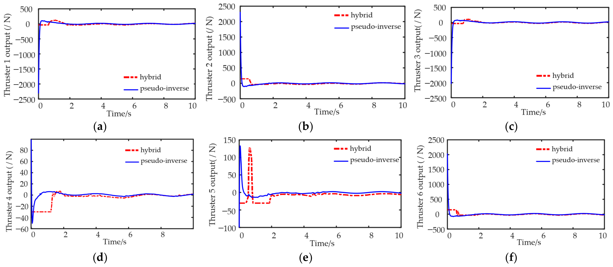
It can be observed that under unknown disturbances, both thrust allocation methods enable the system to stabilize at the target angles, thereby achieving attitude control. Figure 6 presents the thruster thrust allocation results obtained using the pseudo-inverse method and the hybrid method combining the improved pseudo-inverse method with the active-set method.

Compared with the pseudo-inverse method, the hybrid method effectively satisfies the requirement of limiting thruster outputs, particularly for Thrusters 1, 2, 3, and 6 during the initial stage, where the thrust limitation plays a notable role. Moreover, the thrust distribution among all thrusters is more balanced with the hybrid method than with the pseudo-inverse method, resulting in a more reasonable allocation of thruster forces. After the attitude angles stabilize, Thrusters 3 and 6 continue to produce sustained thrust outputs. This is because, in the presence of nonzero attitude angles, the thrusters must continuously work to overcome the restoring moments. Upon analyzing the attitude angle responses, it is found that the pseudo-inverse method achieves faster attitude stabilization. This is attributed to the fact that the thrust solutions obtained via the pseudo-inverse method lead to faster vehicle motion, albeit without accounting for thruster output constraints. In contrast, the hybrid method yields a slower stabilization speed; however, it effectively avoids severe thrust exceedance during the initial stage and produces more evenly distributed thruster outputs, thereby significantly alleviating thruster saturation.

4.2. Depth-Holding Control Simulation

The underwater depth-holding control simulation is configured as follows. The initial position and attitude of the ROV are set to zero, after which the vehicle performs depth-holding motion to approach and stabilize at the target depth. To emulate the real underwater operational environment, two types of typical disturbances are applied under still-water conditions: (1) a time-varying pulsating disturbance arising from thruster fluctuations and ambient wave-induced oscillations, and (2) a vertical disturbance force induced by tether drag. The total disturbance force is expressed as:

$$D_f=50\sin (2\pi t/350)\times \sin (2\pi t/280)\times \sin (2\pi t/150)+{\displaystyle \frac{1}{2}}\rho d{C}_n{w}^2\sin \psi \sin \left|\psi \right|$$

(54)

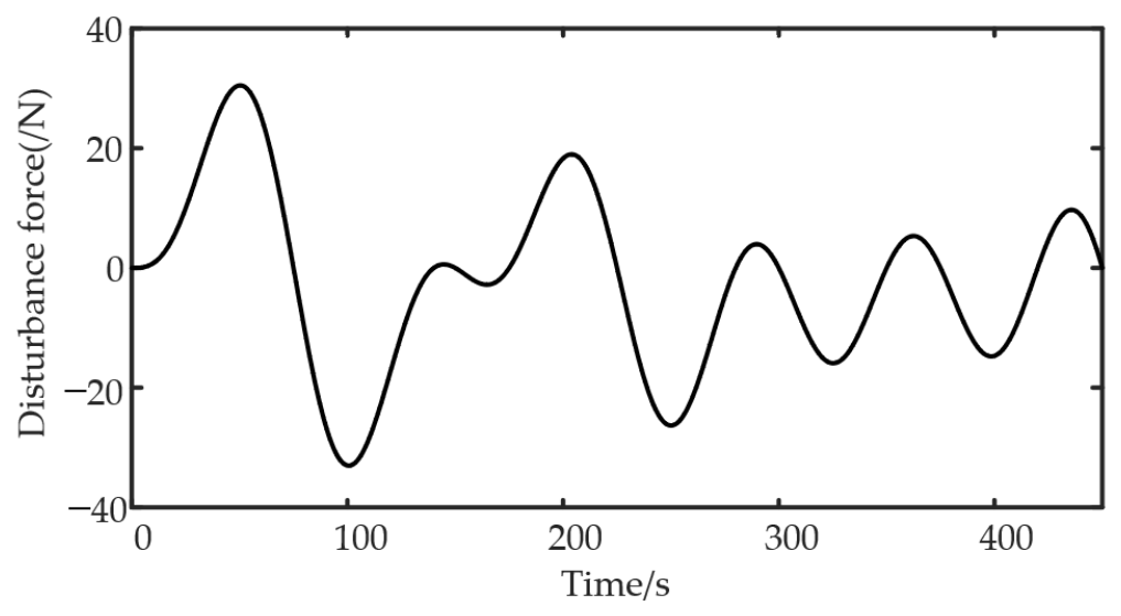
The first term is a triple-frequency product-type time-varying disturbance, which can approximately simulate the nonlinear coupling effects of multi-source low-frequency environmental disturbances such as ocean currents and internal waves. The second term, constructed based on Morison’s equation, describes the normal drag force exerted by the tether on the ROV, where $\rho$ denotes the fluid density, $d$ is the tether diameter, $C_n$ is the normal drag coefficient, $\psi$ is the angle of attack of the tether relative to the incoming flow, which is set to 90° to maximize the vertical drag component, and $\omega$ is the heave velocity of the ROV calculated according to the maximum design speed of 0.2 m/s. This disturbance model preserves complex time-domain variation characteristics and can effectively evaluate the robustness of the controller under multi-source time-varying disturbances. Disturbance force variation curves are shown in Figure 7. The depth-holding controller parameters are listed in

Table 2. Parameters of the depth-holding controller.

B-ASMC		PID
Parameter	Value	Parameter	Value
$c$	20	$K_P$	5
$h$	20	$K_I$	0
$k$	20	$K_D$	1
$\gamma$	3

.

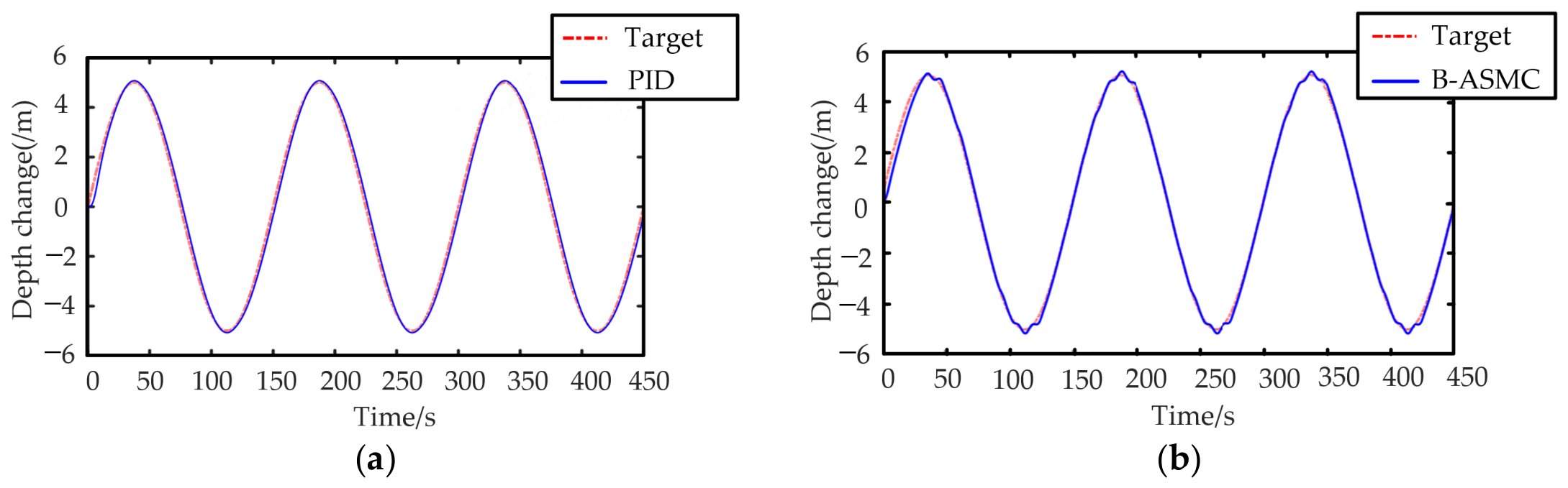
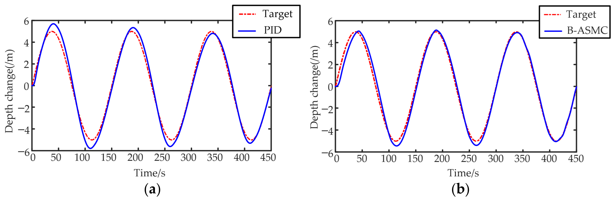
A time-varying reference signal is used to evaluate the dynamic performance of the two controllers. The reference signal is a sinusoidal function with an amplitude of 5 m and a frequency of $2\times pi/150$. The sampling time is 0.01 s; the simulation uses a fixed-step discrete solver with a fixed step size of 0.01 s, and the simulation duration is 450 s. The ROV depth change responses of PID and B-ASMC are shown in Figure 8 and Figure 9.

The simulation results show that both control methods can track the desired depth under both disturbance-free and disturbed conditions. In terms of signal-tracking performance, the PID controller produces a relatively smooth depth response, but it is overly smoothed near peaks and troughs where the signal variation rate is large. In contrast, B-ASMC exhibits slight vibration near peaks and troughs, which affects local tracking quality; however, its tracking remains smooth during the other motion phases. Under disturbances, the control performance of both PID and B-ASMC deteriorates markedly, but B-ASMC still maintains a satisfactory tracking capability.

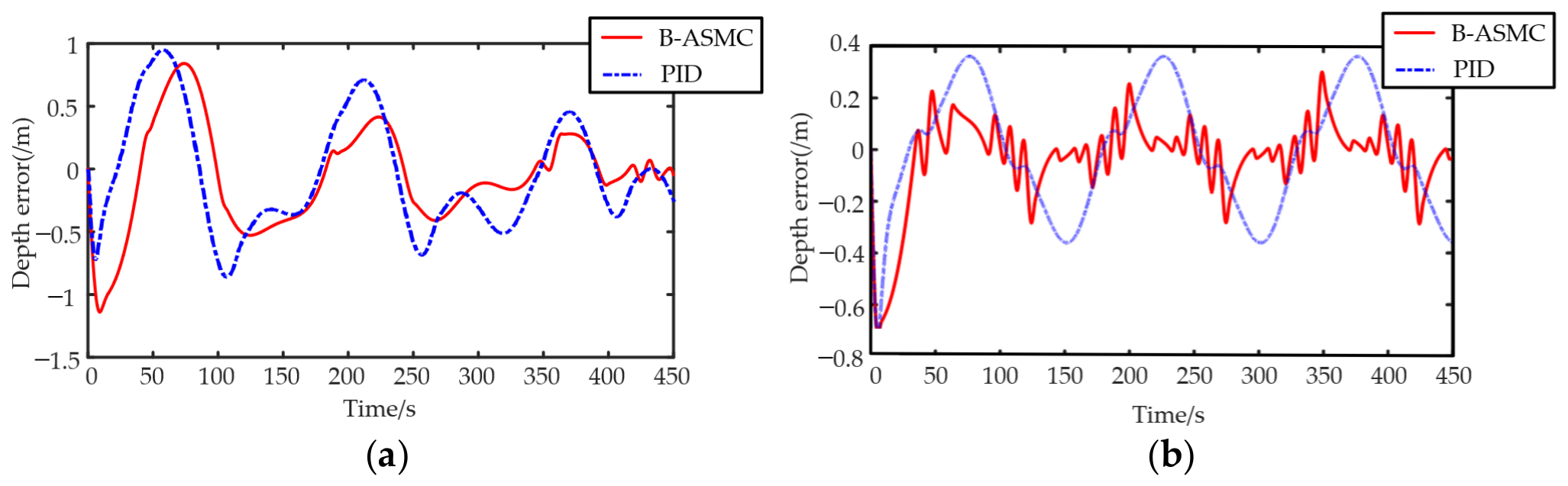
The depth errors are shown in Figure 10. The mean square error and root mean square error are used to quantify the tracking-error levels of the two controllers. Without disturbances, the PID errors are 0.0557 and 0.2361, whereas the B-ASMC errors are 0.0271 and 0.1648, respectively, indicating that B-ASMC achieves lower errors than PID. Under disturbances, the PID errors increase to 0.2072 and 0.4552, whereas the B-ASMC errors are 0.1586 and 0.3983. Therefore, although control performance degrades under unknown time-varying disturbances, B-ASMC consistently outperforms PID.

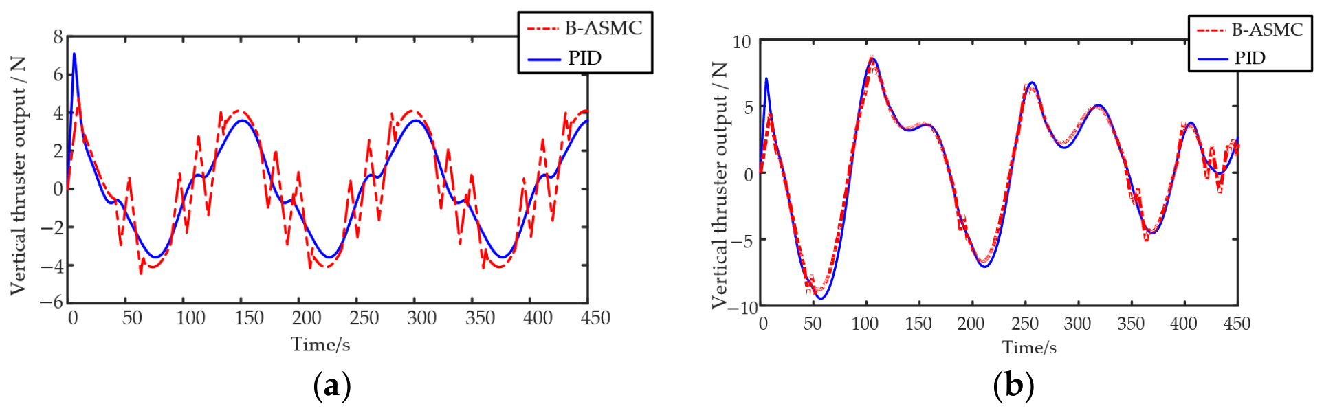
The hybrid thrust allocation strategy proposed in the preceding section is adopted in this simulation. Under single-degree-of-freedom actuation, it follows from the thrust allocation model of the ROV propulsion system that only the four vertical thrusters are active during depth control, and the output thrust of these four thrusters is identical. The resulting thruster output variations are presented in Figure 11.

A comparison of the thruster outputs in the simulations reveals that, under disturbance-free conditions, the PID exhibits a pronounced jump at the initial stage and requires a longer settling time, although it eventually achieves complete stabilization. In contrast, the B-ASMC produces relatively mild thrust fluctuations and reaches the steady state more quickly; however, it exhibits output oscillations due to the chattering phenomenon that cannot be entirely eliminated. Under disturbed conditions, the overall variation trends of the thruster outputs for both controllers are similar.

4.3. Bow Heading-Holding Control Simulation

The underwater bow heading-holding control simulation is configured as follows. The initial position and attitude of the ROV are set to zero, after which the vehicle performs heading-holding motion to approach and stabilize at the target heading angle. To emulate the real underwater operational environment, two types of typical disturbances are applied under still-water conditions: a time-varying pulsating disturbance arising from thruster fluctuations and ambient wave-induced oscillations, and a heading disturbance moment induced by tether drag. The total disturbance is expressed as:

$$D_f=15\sin (2\pi t/350)\times \sin (2\pi t/200)\times \sin (2\pi t/100)+{\displaystyle \frac{1}{2}}l\rho d{C}_n{r}^2\sin \psi \sin \left|\psi \right|$$

(55)

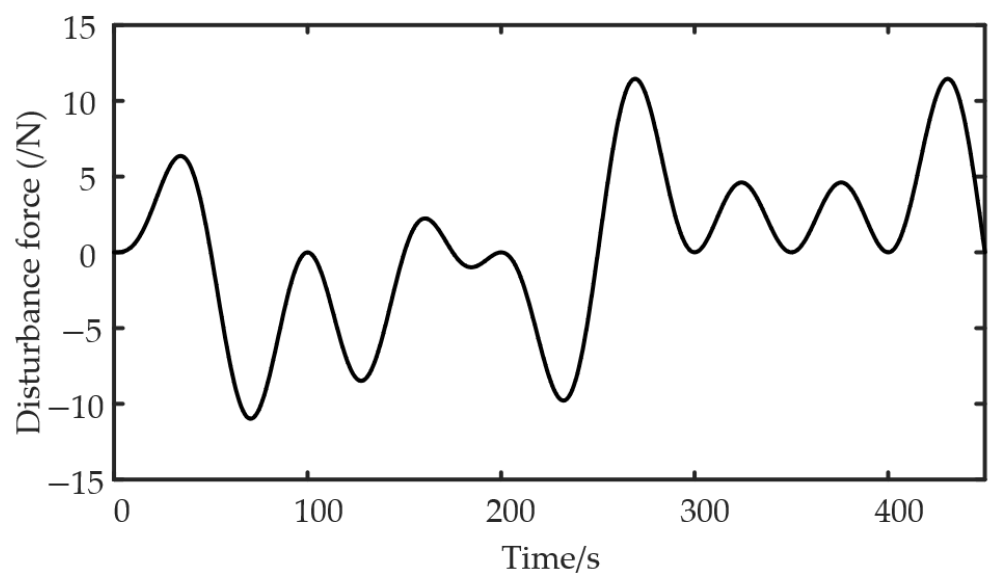
This disturbance model is designed similarly to that of the depth-holding case. Owing to the smaller moment of inertia in the yaw direction, the heading control loop exhibits faster response and greater sensitivity to time-varying disturbances. Consequently, the pulsating disturbance amplitude is set lower while the frequency components are set higher compared with the depth-holding case. The second term is similarly constructed based on Morison’s equation to describe the yaw resistance moment exerted by the tether on the ROV, where $\psi$ is the angle of attack of the tether relative to the incoming flow, which is set to 90° to maximize the yaw disturbance moment component, and $r$ is the yaw angular velocity of the ROV set to 0.1 rad/s. Disturbance force variation curves are shown in Figure 12. The bow heading-holding controller parameters are listed in

Table 3. Parameters of the bow heading-holding controller.

B-ASMC		PID
Parameter	Value	Parameter	Value
$c$	20	$K_P$	0.1
$h$	20	$K_I$	0
$k$	20	$K_D$	0.01
$\gamma$	3

.

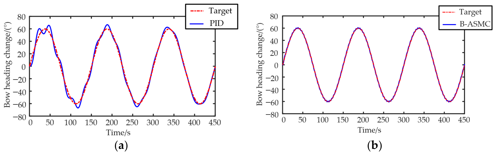
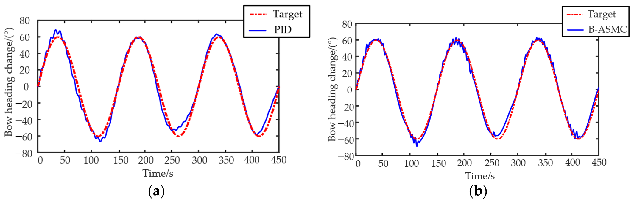
A time-varying reference signal is used to evaluate the dynamic performance of the two controllers. The reference signal is a sinusoidal function with an amplitude of 60 and a frequency of $2\times pi/150$. The sampling time is 0.01 s; the simulation uses a fixed-step discrete solver with a fixed step size of 0.01 s, and the simulation duration is 450 s. The ROV bow heading responses of PID and B-ASMC are shown in Figure 13 and Figure 14.

Both control methods can track the desired bow heading. In terms of signal tracking, the bow heading change response under PID cannot closely follow the target signal and varies relatively slowly, whereas B-ASMC provides better tracking performance but still exhibits high-frequency vibration. Under time-varying disturbances, the bow heading-tracking performance of both PID and B-ASMC decreases, and B-ASMC shows slight vibration near the peaks and troughs.

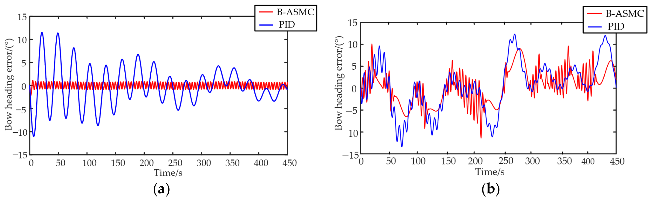
The depth errors are shown in Figure 15; it is observed that PID requires parameter retuning, whereas B-ASMC maintains good control performance under unknown time-varying disturbances without retuning, demonstrating strong robustness to such disturbances. The bow heading tracking errors are shown in Figure 10. The mean square error and root mean square error are again used to quantify the tracking-error levels. Without disturbances, the PID errors are 17.3412 and 4.1644, whereas the B-ASMC errors are 0.3339 and 0.5778, respectively. Under disturbances, the PID errors are 31.1590 and 5.5820, whereas the B-ASMC errors are 15.6058 and 3.9504. Thus, B-ASMC consistently outperforms PID regardless of whether disturbances are present.

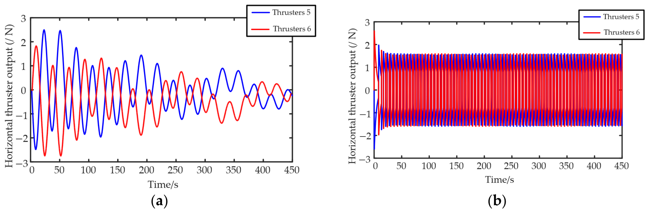
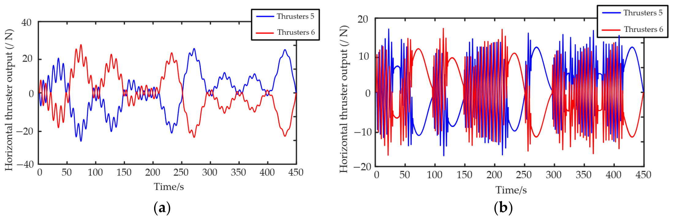
The hybrid thrust allocation strategy is also adopted in this case. The directional control is primarily achieved through Thrusters 5 and 6, with the corresponding thruster output variations presented in Figure 16 and Figure 17.

The two horizontal thrusters operate in a complementary manner, with the output thrust of each remaining within the thruster capability limits. Under disturbance-free conditions, the PID produces smoother output signals, whereas the B-ASMC exhibits higher-frequency variations in the output signals. Under time-varying disturbances, the results are consistent with those described previously.

5. Experimental Validation

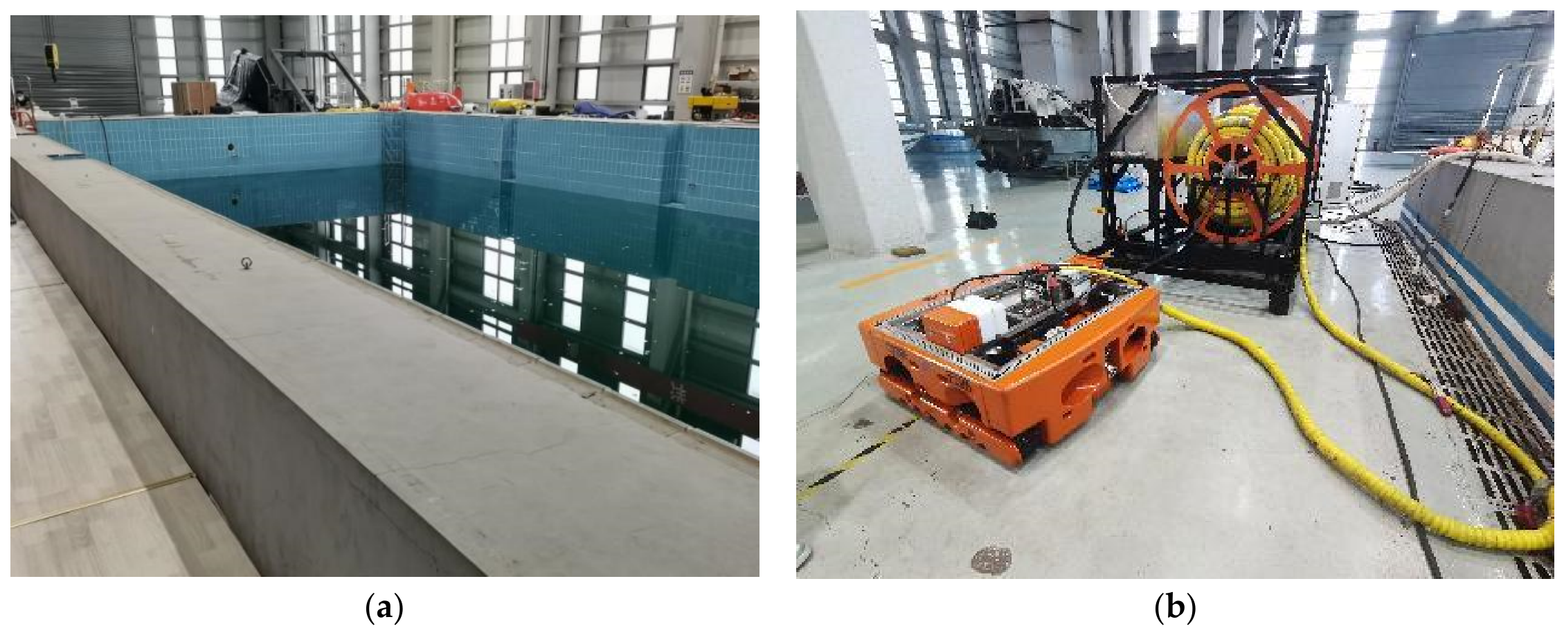
The control algorithm validated through simulation is implemented as embedded code, and ROV depth-holding and bow heading-holding experiments are conducted in an indoor pool. The ROV experimental platform is shown in Figure 18; the pool is 30 m × 10 m × 10 m. The control system uses a depth sensor as the feedback signal for depth-holding control. The pitch angle of the ROV is regulated according to the depth difference between the two sensors. Meanwhile, a high-performance inertial measurement unit was used to provide attitude feedback. Every 0.5 s, the depth-holding data and inertial measurement data are collected, packaged, and transmitted to both the controller program and the host–computer interface, where the feedback data are recorded and plotted.

5.1. ROV Depth-Holding Control

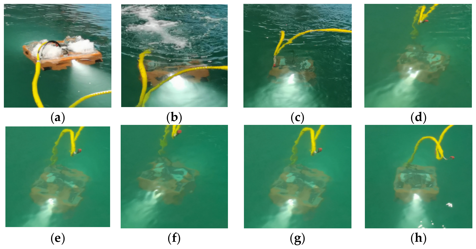
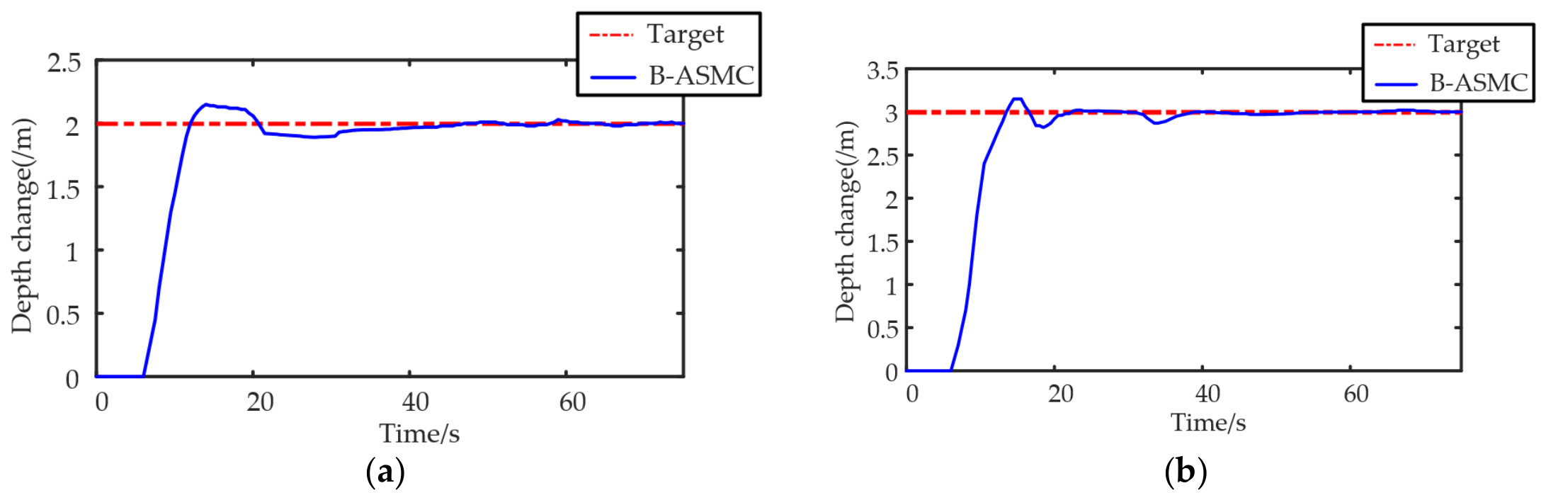
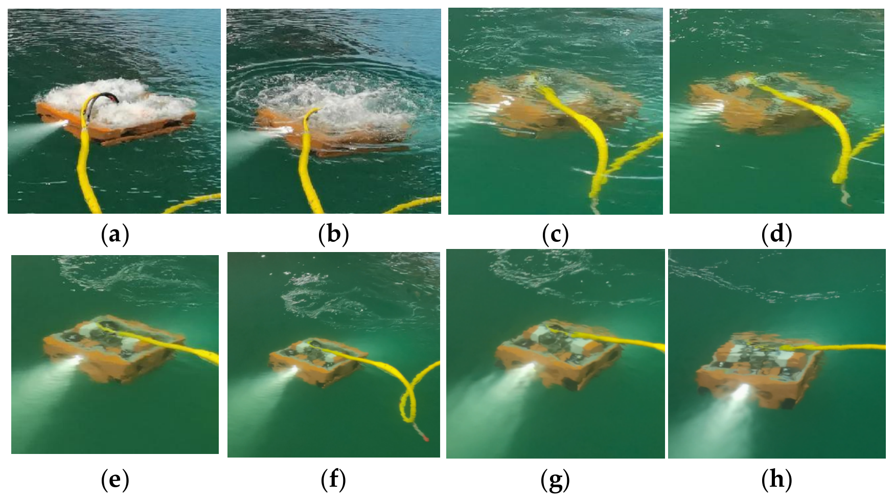
The desired depth was set, and the depth-holding function was activated. A depth target of 2 m is first assigned to the ROV, and the experimental process is shown in Figure 19. A second depth target of 3 m is then assigned, and the corresponding experimental process is shown in Figure 20.

The recorded depth variations during the ROV depth-holding experiments are shown in Figure 21. During the experiments, the jet disturbance generated by the thrusters, waves in the pool, and tether forces induce noticeable longitudinal and lateral displacement of the ROV. Nevertheless, the ROV stabilizes rapidly at the target depth. B-ASMC ultimately achieves reliable depth control, demonstrating its effectiveness and robustness against unknown disturbances.

5.2. ROV Bow Heading-Holding Control

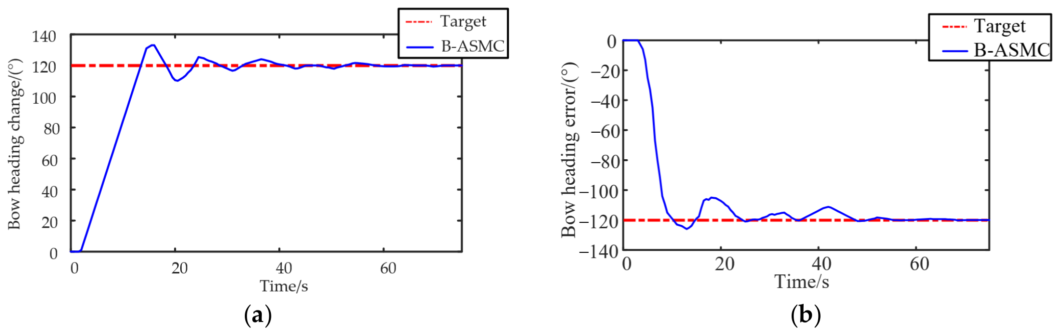
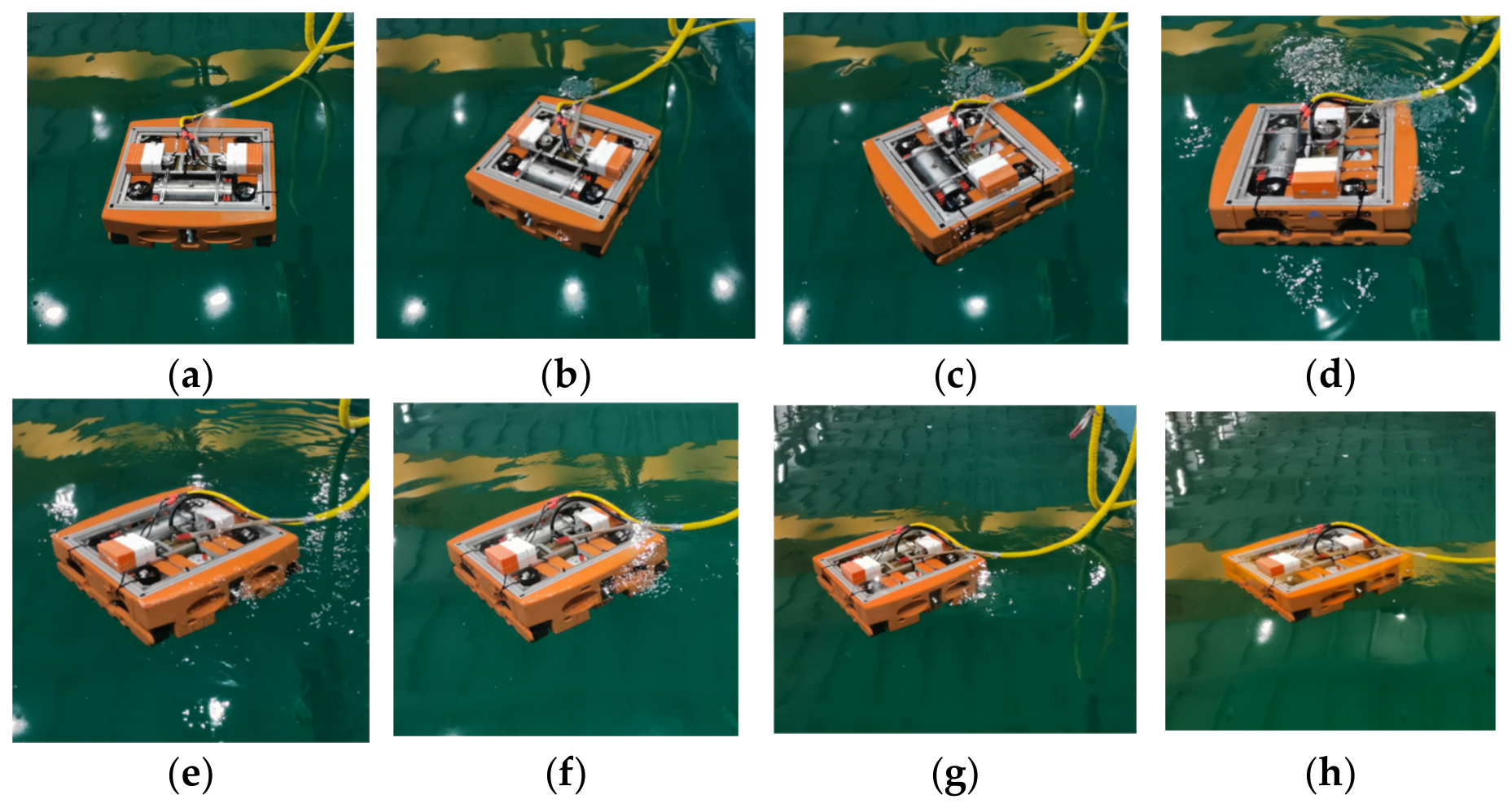
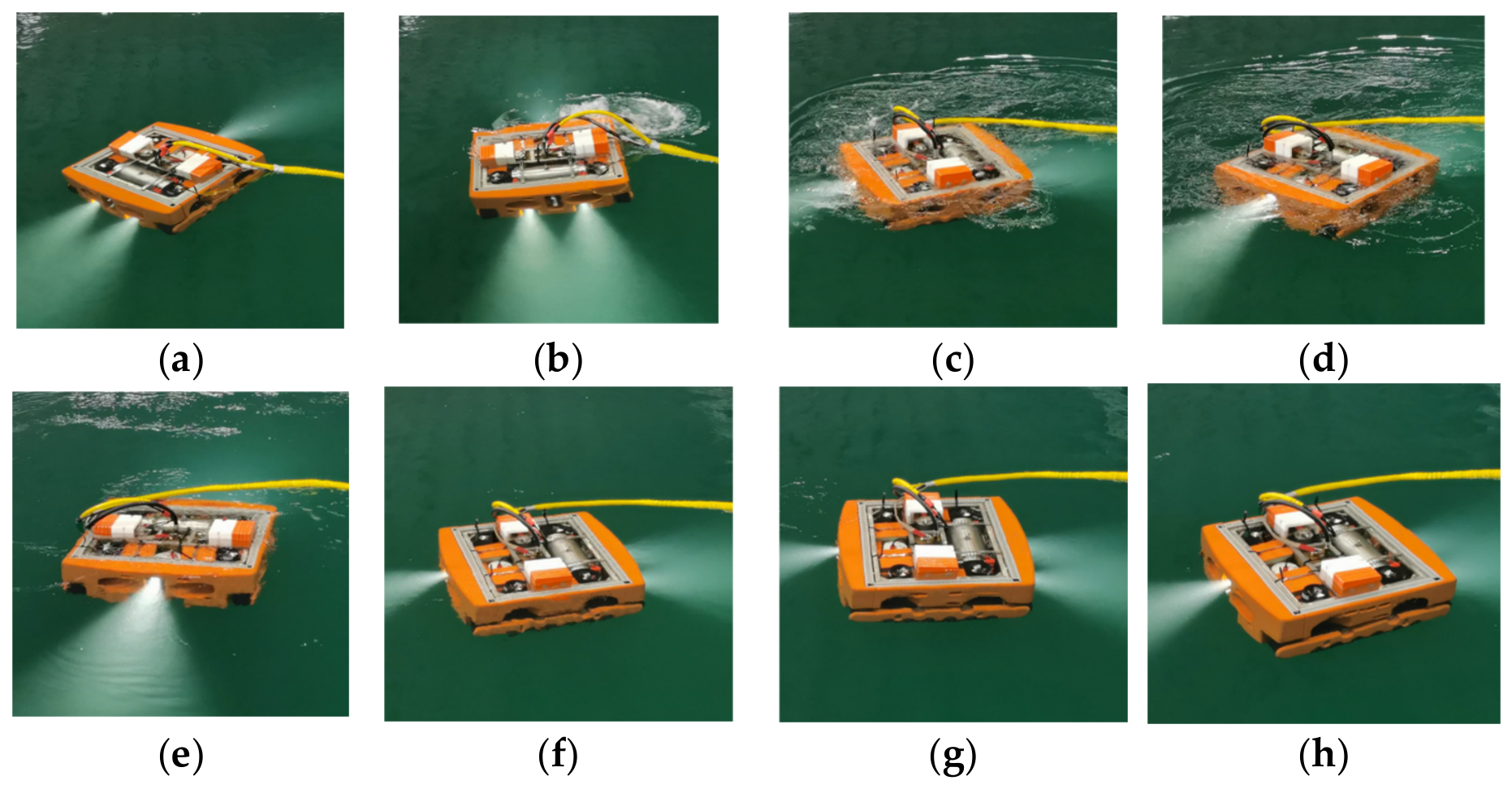
The host computer sets the target depth and activates the depth-holding function. Two bow heading-holding cases are then tested: (1) an initial bow heading of 0° with a target bow heading of 120°, and (2) an initial bow heading of 0° with a target bow heading of −120°. The experimental processes are shown in Figure 22 and Figure 23. The recorded bow heading variations are shown in Figure 18 and Figure 24. The ROV ultimately stabilizes at −120° and 120°, respectively. During the experiments, the ROV is affected by wave disturbances in the pool and by tether forces. Considering the overall 0.5 s delay of the ROV control system, the slight wave disturbances in the pool, and the tether-induced disturbances acting on the ROV, B-ASMC still achieves effective bow heading-holding control, thereby validating the effectiveness of the proposed method.

6. Conclusions

To address the high-precision motion control problem of ROVs operating in complex environments, this study proposed a B-ASMC method and designed a hybrid thrust allocation strategy based on the pseudo-inverse and active-set methods. The proposed controller integrates the systematic design framework of backstepping control with the strong robustness of sliding mode control. By introducing an adaptive law to estimate the lumped system disturbance online, it avoids reliance on an accurate disturbance observer or an exact system model, reduces the need for prior knowledge of the disturbance upper bound, and rigorously establishes the global asymptotic stability of the closed-loop system using Lyapunov stability theory. Simulation and pool-experiment results demonstrate that, compared with PID control, the proposed B-ASMC achieves higher tracking accuracy, faster response, and stronger disturbance rejection under both depth-holding and bow heading-holding conditions. Future work will extend the proposed framework to the full trajectory tracking problem in spatially varying flow fields, introduce neural network-based disturbance prediction to further improve transient performance, and conduct open-water sea trials under more severe sea conditions to achieve fully autonomous adaptive operations in unknown and changing underwater environments.

References

1. Schultz, M.P. Effects of coating roughness and biofouling on ship resistance and powering. Biofouling 2007, 23, 331–341. [Google Scholar] [CrossRef] [Scilit] [PubMed]
2. Chen, L.; Cui, R.; Yan, W.; Xu, H.; Zhao, H.; Li, H. Design and climbing control of an underwater robot for ship hull cleaning. Ocean Eng. 2023, 274, 114024. [Google Scholar] [CrossRef] [Scilit]
3. Fossen, T.I. Handbook of Marine Craft Hydrodynamics and Motion Control; John Wiley & Sons: Chichester, UK, 2011. [Google Scholar] [CrossRef] [Scilit]
4. Guo, Y.; Yu, X.; Guo, S.; Liu, X.; Kong, Y.; Li, M.; Chen, W. Analysis on ROV dynamic responses under considerations of moving boundary and coupling hydrodynamic force. Nonlinear Dyn. 2025, 113, 8003–8018. [Google Scholar] [CrossRef] [Scilit]
5. Llorente-Vidrio, D.; Chavez-Galaviz, J.; Fuentes-Aguilar, R.Q.; Chairez, I.; Mahmoudian, N. Robust sliding-mode control of an underwater ROV via neural differential identification of model uncertainties. Ocean Eng. 2025, 341, 122728. [Google Scholar] [CrossRef] [Scilit]
6. Chen, Y.; Miao, Z.; Wei, J.; Wang, Y.; Gao, T.; He, W.; Wang, H. Dual-loop safety control for underwater vehicles: Obstacle avoidance and disturbance rejection. IEEE/ASME Trans. Mechatron. 2026, 31, 2112–2123. [Google Scholar] [CrossRef] [Scilit]
7. Chen, H.; Tang, G.; Xiao, W.; Zhou, X.; Wu, D.; Gui, L. K∞ function-based robust sliding mode control for remotely operated vehicles: Theory, simulations, and experiments. Control Eng. Pract. 2024, 156, 106230. [Google Scholar] [CrossRef] [Scilit]
8. Vo, A.T.; Truong, T.N.; Hong, I.P.; Kang, H.J. Sliding mode control method based on a fuzzy logic system for ROVs with predefined-time convergence and stability. Mathematics 2025, 13, 1573. [Google Scholar] [CrossRef] [Scilit]
9. Xia, T.; Yang, Q.; Zheng, Y.; Huang, B.; Ouyang, Y. Trajectory tracking control of work-class ROVs using KORMPC strategy. Ocean Eng. 2025, 341, 122801. [Google Scholar] [CrossRef] [Scilit]
10. Yang, G.; Liu, W.; Li, L.; Xu, J.; Guo, L.; Zhang, K. Optimized trajectory tracking for ROVs using DNN + ENMPC strategy. J. Mar. Sci. Eng. 2024, 12, 1827. [Google Scholar] [CrossRef] [Scilit]
11. Utkin, V. Variable structure systems with sliding modes. IEEE Trans. Autom. Control 1977, 22, 212–222. [Google Scholar] [CrossRef] [Scilit]
12. Truong, T.N.; Vo, A.T.; Kang, H.J. A model-free fixed-time terminal sliding mode control method for robot systems. In Proceedings of the 2024 17th International Workshop on Variable Structure Systems (VSS); IEEE: Abu Dhabi, United Arab Emirates, 2024; pp. 184–189. [Google Scholar] [CrossRef] [Scilit]
13. Huang, B.; Yang, Q. Double-loop sliding mode controller with a novel switching term for the trajectory tracking of work-class ROVs. Ocean Eng. 2019, 178, 80–94. [Google Scholar] [CrossRef] [Scilit]
14. Luo, G.; Gao, S.; Jiang, Z.; Luo, C.; Zhang, W.; Wang, H. ROV trajectory tracking control based on disturbance observer and combinatorial reaching law of sliding mode. Ocean Eng. 2024, 304, 117744. [Google Scholar] [CrossRef] [Scilit]
15. Deng, L.; Tao, J. Fractional-order sliding mode control for a remotely operated vehicle with saturated input constraints. IEEE Access 2025, 13, 51669–51679. [Google Scholar] [CrossRef] [Scilit]
16. Kim, M.; Joe, H.; Kim, J.; Yu, S.C. Integral sliding mode controller for precise manoeuvring of autonomous underwater vehicle in the presence of unknown environmental disturbances. Int. J. Control 2015, 88, 2055–2065. [Google Scholar] [CrossRef] [Scilit]
17. Chen, Y.; Li, J.; Zhang, H.; Dai, R.; Gu, Y. Design of model-free sliding mode controller for ROV based on neural dynamics model. Ocean Eng. 2026, 347, 124022. [Google Scholar] [CrossRef] [Scilit]
18. Krstic, M.; Kanellakopoulos, I.; Kokotovic, P.V. Nonlinear and Adaptive Control Design; John Wiley & Sons: New York, NY, USA, 1995. [Google Scholar]
19. Raygosa-Barahona, R.; Parra-Vega, V.; Olguin-Diaz, E.; Muñoz-Ubando, L. A model-free backstepping with integral sliding mode control for underactuated ROVs. In Proceedings of the 2011 8th International Conference on Electrical Engineering, Computing Science and Automatic Control (CCE); IEEE: Merida, Mexico, 2011; pp. 1–7. [Google Scholar] [CrossRef] [Scilit]
20. Chen, Q.; Yuan, J.; Dong, Z.; Chai, Z.; Wan, L. Enhanced control strategies for underactuated AUVs using backstepping integral sliding mode techniques for ocean current challenges. J. Mar. Sci. Eng. 2024, 12, 2201. [Google Scholar] [CrossRef] [Scilit]
21. Teji, M.D.; Zou, T.; Zeleke, D.S. Backstepping-Based Nonsingular Terminal Sliding Mode Control for Finite-Time Trajectory Tracking of a Skid-Steer Mobile Robot. Robotics 2024, 13, 180. [Google Scholar] [CrossRef] [Scilit]
22. Liu, X.; Sun, B.; Su, Z. Adaptive sliding mode control for AUV based on backstepping and neural networks. Meas. Sci. Technol. 2024, 35, 016215. [Google Scholar] [CrossRef] [Scilit]
23. Tang, S.; Xue, N.; Liu, K.; Wang, D.; Ye, J.; Fan, T. Motion control for an open-frame work-class ROV in current using an adaptive super-twisting disturbance observer. Ocean Eng. 2023, 280, 114723. [Google Scholar] [CrossRef] [Scilit]
24. Zhao, Y.; Xu, S.; Zheng, X.; Luo, L.; Xu, B.; Xiong, C. Enhanced real-time simulation of ROV attitude and trajectory under ocean current and wake disturbances. Appl. Syst. Innov. 2025, 8, 75. [Google Scholar] [CrossRef] [Scilit]
25. Li, X.; Zhao, M.; Ge, T. A nonlinear observer for remotely operated vehicles with cable effect in ocean currents. Appl. Sci. 2018, 8, 867. [Google Scholar] [CrossRef] [Scilit]
26. Pei, X.; Gu, X.; Zou, Y. Research on Attitude Control of Cable Underwater Cleaning Robot. In Proceedings of the 2024 IEEE International Conference on Mechatronics and Automation (ICMA), Tianjin, China, 4–7 August 2024; pp. 228–233. [Google Scholar] [CrossRef] [Scilit]
27. Baldini, A.; Fasano, A.; Felicetti, R.; Freddi, A.; Longhi, S.; Monteriù, A. A constrained thrust allocation algorithm for remotely operated vehicles. IFAC-PapersOnLine 2018, 51, 250–255. [Google Scholar] [CrossRef] [Scilit]
Figure 1. Definition of the body-fixed and earth-fixed coordinate frames.
Robotics 15 00173 g001
Figure 2. Schematic of the thruster configuration. (a) Horizontal thruster configuration. (b) Vertical thruster configuration.
Robotics 15 00173 g002
Figure 3. Schematic of the thrust allocation system.
Robotics 15 00173 g003
Figure 4. Motion control simulation scheme.
Robotics 15 00173 g004
Figure 5. Attitude angle variations under the pseudo-inverse method and the hybrid thrust allocation strategy combining the improved pseudo-inverse method with the active-set method. (a) Roll. (b) Pitch. (c) Yaw.
Robotics 15 00173 g005
Figure 6. Thruster thrust allocation results obtained using the pseudo-inverse method and the hybrid method that combines the improved pseudo-inverse method with the active-set method. (a) Thruster 1. (b) Thruster 2. (c) Thruster 3. (d) Thruster 4. (e) Thruster 5. (f) Thruster 6.
Robotics 15 00173 g006
Figure 7. Disturbance force variation under depth-holding control.
Robotics 15 00173 g007
Figure 8. Depth change response of PID and B-ASMC under disturbance-free conditions. (a) Depth change response of PID. (b) Depth change response of B-ASMC.
Robotics 15 00173 g008
Figure 9. Depth change response of PID and B-ASMC under disturbance condition. (a) Depth change response of PID. (b) Depth change response of B-ASMC.
Robotics 15 00173 g009
Figure 10. Depth error of B-ASMC and PID. (a) Disturbance-free condition. (b) Disturbed condition.
Robotics 15 00173 g010
Figure 11. Vertical thruster output under B-ASMC and PID. (a) Disturbance-free condition. (b) Disturbed condition.
Robotics 15 00173 g011
Figure 12. Disturbance force variation under bow heading-holding control.
Robotics 15 00173 g012
Figure 13. Bow heading change response of PID and B-ASMC under disturbance-free conditions. (a) Bow heading change response of PID. (b) Bow heading change response of B-ASMC.
Robotics 15 00173 g013
Figure 14. Bow heading change response of PID and B-ASMC under disturbance conditions. (a) Bow heading change response of PID. (b) Bow heading change response of B-ASMC.
Robotics 15 00173 g014
Figure 15. Bow heading error of B-ASMC and PID. (a) Disturbance-free condition. (b) Disturbed condition.
Robotics 15 00173 g015
Figure 16. Horizontal thruster output of thruster 5 and thruster 6 under disturbance-free conditions. (a) PID. (b) B-ASMC.
Robotics 15 00173 g016
Figure 17. Horizontal thruster output of thruster 5 and thruster 6 under disturbance conditions. (a) PID. (b) B-ASMC.
Robotics 15 00173 g017
Figure 18. ROV experimental platform. (a) ROV experimental tank. (b) Umbilical cable connection before ROV immersion.
Robotics 15 00173 g018
Figure 19. Experimental performance of ROV depth-holding control at 2 m over different time periods. (a) 5 s. (b) 10 s. (c) 15 s. (d) 20 s. (e) 25 s. (f) 30 s. (g) 35 s. (h) 40 s.
Robotics 15 00173 g019
Figure 20. Experimental performance of ROV depth-holding control at 3 m over different time periods. (a) 5 s. (b) 10 s. (c) 15 s. (d) 20 s. (e) 25 s. (f) 30 s. (g) 35 s. (h) 40 s.
Robotics 15 00173 g020
Figure 21. Depth change response of B-ASMC. (a) Depth-holding control at 2 m. (b) Depth-holding control at 3 m.
Robotics 15 00173 g021
Figure 22. Experimental performance of ROV bow heading-holding control from 0° to 120° over different time periods. (a) 5 s. (b) 10 s. (c) 15 s. (d) 20 s. (e) 25 s. (f) 30 s. (g) 35 s. (h) 40 s.
Robotics 15 00173 g022
Figure 23. Experimental performance of ROV bow heading-holding control from 0° to −120° over different time periods. (a) 5 s. (b) 10 s. (c) 15 s. (d) 20 s. (e) 25 s. (f) 30 s. (g) 35 s. (h) 40 s.
Robotics 15 00173 g023
Figure 24. Bow heading change response of B-ASMC. (a) Bow heading-holding control from 0° to 120°. (b) Bow heading-holding control from 0° to −120°.
Robotics 15 00173 g024