Abstract
This work introduces a unified Artificial Intelligence-based framework for the optimal tuning of gains in a neural discrete-time sliding mode controller (SMC) applied to a two-degree-of-freedom robotic manipulator. The novelty lies in combining surrogate-assisted optimization with normalized search spaces to enable a fair comparative analysis of three metaheuristic strategies: Bayesian Optimization (BO), Particle Swarm Optimization (PSO), and Genetic Algorithms (GAs). The manipulator dynamics are identified via a discrete-time recurrent high-order neural network (NN) trained online using an Extended Kalman Filter with adaptive noise covariance updates, allowing the model to accurately capture unmodeled dynamics, nonlinearities, parametric variations, and process/measurement noise. This neural representation serves as the predictive plant for the discrete-time SMC, enabling precise control of joint angular positions under sinusoidal phase-shifted references. To construct the optimization dataset, MATLAB® simulations sweep the controller gains over a bounded physical domain, logging steady-state tracking errors. These are normalized to mitigate scaling effects and improve convergence stability. Optimization is executed in Python® using integrated scikit-learn, DEAP, and scikit-optimize routines. Simulation results reveal that all three algorithms reach high-performance gain configurations. Here, the combined cost is the normalized aggregate objective constructed from the steady-state tracking errors of both joints. Under identical experimental conditions (shared data loading/normalization and a single Python pipeline), PSO attains the lowest error in Joint 1 ( rad) with the shortest runtime (23.44 s); GA yields the lowest error in Joint 2 ( rad) at higher computational expense (≈69.7 s including refinement); and BO is competitive in both joints ( rad, rad) with a runtime comparable to PSO (23.65 s) while using only 50 evaluations.
1. Introduction
Neural sliding mode control (SMC) has become an effective paradigm for dealing with the nonlinearities and uncertainties inherent in robotic systems. In particular, discrete-time formulations of SMC combined with neural approximators have gained attention for real-time control applications involving robotic manipulators. However, the tuning of control gains in these architectures remains a non-trivial task that directly influences performance, robustness, and stability.
Recent contributions in the literature have explored a variety of approaches to optimize sliding mode controller parameters using nature-inspired and learning-based strategies. For example, in [1], a robust adaptive neural SMC framework was proposed, optimized via Grey Wolf Optimizer to enhance tracking accuracy and robustness in robot manipulators.
Similarly, in [2], a Particle Swarm Optimization (PSO)-tuned SMC was implemented in the context of robotic rehabilitation, highlighting its effectiveness for human–robot interaction. Within physical human–robot collaboration (pHRC), recent work has modeled a robot’s trust in its human co-worker using measurable factors, validated on a collaborative manipulator setup [3]. Other researchers have focused on Bayesian-based strategies, such as adaptive Gaussian process modeling with adaptive kernels to improve sample efficiency in robotic control scenarios [4]. Genetic Algorithms (GAs) have also been investigated for gain optimization in SMC settings; for instance, [5] demonstrated the effectiveness of GA-tuned SMC in mitigating chattering and ensuring precision tracking in multi-DOF manipulators.
Beyond traditional metaheuristics, recent advances have incorporated Artificial Intelligence techniques into the sliding mode framework. For example, in [6], an adaptive neural sliding mode controller for a flexible robotic manipulator was proposed, where the neural network learns online to approximate model uncertainties, ensuring robust tracking despite dynamic variations. In a related direction, in [7], a deep reinforcement learning-based SMC design was introduced for a partially known nonlinear systems, in which a policy gradient method adaptively adjusts the sliding mode control effort, effectively bridging classical robustness with data-driven adaptability. Complementarily, sampled-data admittance control integrated with a data-driven moving-horizon velocity estimator (based on Willems’ fundamental lemma) has been shown to stabilize pHRI under noisy, discontinuous velocity measurements and to improve both transient and steady-state tracking [8].
Despite recent advances in Artificial Intelligence (AI)-based controller design, most studies either focus on continuous-time implementations or lack a unified methodology for comparing multiple optimization strategies under the same normalized framework. Moreover, few works incorporate a surrogate modeling strategy to reduce computational cost during optimization iterations. Also, in real-world control applications, the tuning of controller gains is frequently performed manually, relying on heuristic adjustments and iterative trial-and-error refinements by human experts. This manual approach is not only time-consuming but also prone to suboptimal performance, especially in systems with nonlinear dynamics, modeling errors, or parametric uncertainties. These challenges are amplified when dealing with discrete-time implementations and neural-based controllers, where interactions between gain parameters and recurrent dynamics are not easily interpretable.
To address this, this work proposes a comprehensive methodology to optimize the gains of a neural discrete-time sliding mode controller using three metaheuristic techniques: Bayesian Optimization (BO), Particle Swarm Optimization (PSO), and Genetic Algorithms (GAs). The robot dynamics are first estimated via a recurrent high-order neural network trained with an Extended Kalman Filter (EKF) algorithm that dynamically updates measurement and process noise covariance matrices and where the training is performed online. Then, a dataset of tracking errors and gains is collected by sweeping controller parameters in the physical domain and subsequently normalized. This normalization ensures that all optimization algorithms operate within a common domain , enabling fair comparison and improved convergence behavior.
The objective is to identify the optimal control gains that minimize steady-state tracking errors in both joints of a 2-DOF robotic manipulator. By leveraging surrogate models and normalized search spaces, this study demonstrates how each optimization method balances accuracy, computational effort, and robustness, offering valuable insights into controller design for robotic applications.
The main contributions of this work are as follows:
- Discrete-time SMC + recurrent high-order NN integration. It is coupled a discrete-time sliding-mode controller with a recurrent high-order neural network identified online via EKF, with adaptive noise covariance updates. This NN reproduces the 2-DOF robot dynamics used by the controller.
- Unified, normalized benchmark across BO/PSO/GA. All optimizers run in the same pipeline (shared data loading, normalized gain space , identical budgets/criteria, common steady-state error objective), enabling a fair, apples-to-apples comparison.
- Surrogate-assisted screening with diagnostics. Integrate GP surrogates and report model adequacy (), evaluation counts, and wall-clock time alongside tracking performance.
- Progression and convergence analytics. Progression plots (early/mid/final) and normalized convergence curves of the aggregate objective are provided to expose exploration–exploitation dynamics and steady-state improvements in discrete time.
- Constraint-aware evaluation. Limits enforced actuator torque via the SMC saturation branch and verifies bounded control actions in simulation, linking optimization outcomes to implementability.
- Actionable guidance. The unified analysis reveals when PSO, BO, or GA is preferable (e.g., PSO is fastest, BO is most sample-efficient, GA is competitive accuracy at higher cost), providing practical guidance for discrete-time SMC with recurrent high-order NN plants.
- Principled alternative to heuristic tuning. Replaced ad hoc trial and error with a reproducible, data-driven pipeline—discrete-time SMC + recurrent high-order NN—optimized under a unified, normalized setup with BO/PSO/GA.
Together, these elements constitute a novel, reproducible benchmarking framework for discrete-time SMC gain tuning with recurrent high-order NN-based plant models in 2-DOF manipulators, extending beyond isolated demonstrations to deliver a systematic methodology and decision-relevant evidence for controller design.
This paper is organized as follows: Section 2 details the proposed methodology, including the discrete-time modeling of the 2-DOF robot manipulator, the identification of the plant using a recurrent high-order NN trained with the EKF, the implementation of the neural discrete-time sliding mode control algorithm, and the organization of the dataset used for training and simulation. It also describes the application of three metaheuristic optimization algorithms—BO, PSO, and GA—for automatic gain tuning. Section 3 presents the main simulation results across the entire dataset, and some tables of the main results, and Section 4 displays a discussion of the findings and their implications.
2. Methodology
2.1. Dynamic Model of the Two-DOF Robotic Manipulator
To show the proposed method, let us describe the mathematical expression of the robot manipulator in general form in continuous time [9,10]:
For the particular case of the two degrees of freedom robot, are the joint positions (rad), are the joint velocities (rad/s), are the applied torques N · m. The inertia matrix is where
With each element of the matrix is in (kg · ); and , and , and , and are the lengths (m), centers of mass (m), mass (kg), and moments of inertia (kg ) of Links 1 and 2, respectively. The Coriolis and centrifugal contributions are expressed in the form where each element is defined as
Note that in this representation, each element already incorporates the velocity terms and therefore directly represents a torque contribution expressed in (N m). The gravity vector is in (N m). The viscous friction is represented by in (N m s) and the Coulomb friction by in (N m).
To illustrate the present proposal, Dynamical Model (1) is discretized using the Euler approximation [11], which facilitates the implementation of the recurrent high-order NN and the discrete-time sliding mode controller. This discretized model results in
where ; ; ; ; , , and T is the sampling step.
This discrete-time Model (4) is used for both simulating the robot’s response and training the recurrent neural network identifier. The parameters used in Expressions (2) through (3), which are essential for simulating the discrete-time model (4), are derived from the study presented in reference [10].
2.2. State Estimation with Recurrent High-Order NN
In this work, the methodology presented in a previous work [12] is employed, where a discrete-time recurrent high-order NN is employed to identify the dynamical behavior of (4). The goal for proposing this neural network is that this NN has the capability to absorb non-modeled dynamics, modeled error, and possible parameter variations that are common in the real system. Additionally, this NN can aid the controller in gaining variations and nonlinear effects in the closed-loop system produced by the reference inputs for tracking proposed in this work. Also, to make indirect control in series-parallel consuration such that the discrete-time sliding mode algorithm acts directly on the neural network structure and so that the NN reproduces the model (4), the outputs of this model track the reference signals. Then, the recurrent high-order NN proposed for this work has the following general structure:
where x denotes the NN state, with as the number of states, are the adaptive synaptic weights, are nonlinear regressors specific to each joint, are linear dynamic contributions linked to the velocity or torque signals. Specifically, to reproduce the dynamics of the 2-DOF robot model in discrete time (4), the following recurrent high-order NN structure is proposed:
where x are the NN state variables, each one estimating the behavior of their corresponding robot states of System (4); the synaptic weight vectors are adaptive online using the EKF, as explained in [12], where the state noise covariance matrix and the associated measurement noise covariance matrix are computed using a time-varying formulation. Synaptic weights are constant parameters to guarantee the controllability of the system; denotes a standard Gaussian random variable of measurement noise, and are the standard deviations; and hyperbolic tangent (tanh) is the activation function. The goal for using the EKF as training algorithm with the time-varying formulation is to reduce or to eliminate the estimation error .
The present formulation of this NN for estimating the plant states combines nonlinear activation function, dynamic contributions of the applied inputs, adaptive estimation using EKF, and Gaussian noise applied to the measurable variables. This is to show a robust and optimal control algorithm based on the NN structure.
2.3. Discrete-Time Sliding Mode Controller
The control algorithm employed in this work is based on the methodology presented in a previous study [12]. However, unlike their approach—which targets a five-degree-of-freedom robotic system—this proposal focuses on a planar robot with only two degrees of freedom. Naturally, this difference entails significant adjustments in aspects such as the neural network architecture, the number of inputs and outputs, and other related parameters.
We use the methodology presented in [12] to control the Model System (4) indirectly through the proposed recurrent high-order NN (6), such that the following NN tracking error vector converges to zero:
where and are the reference signals to be tracked by the NN states and of System (6), respectively, and therefore by the robot states and of System (4), we follow the methodology presented in [12]. Therefore, the discrete-time sliding mode control law is as follows:
with the discrete control torque vector given by:
In (8), denotes the ith component of the equivalent control vector , computed in (9). The scalar is the actuator torque bound (N · m) for joint i; in these simulations, N · m and N · m. The term is the sign of (and is defined as 0 when ), ensuring pointwise saturation of the torque to the interval .
Also,
with the equivalent control component computed as
and the reference signals
The desired discrete velocity signal is computed as
where
and denotes the estimated dynamic term provided by the recurrent NN identification:
The reference trajectories are defined as
for the step :
and for the step :
where T is the sampling period. It is worth noting that the reference signals assigned to each joint differ in both amplitude and phase. This design choice is intentional and serves to evaluate the stability margin of the proposed control system under non-identical and time-varying tracking conditions. By introducing distinct dynamics for each joint, the control system is subjected to more demanding scenarios, thereby allowing for a more comprehensive assessment of its performance and adaptability. For a more detailed explanation of the control synthesis, please refer to [12].
It is important to remark that the control gains in (14) and in (10) are responsible for driving the NN-based tracking error vector (7) toward zero. Typically, these control gains are tuned heuristically, where the practitioner manually adjusts the parameters based on qualitative or quantitative assessments of the tracking performance. The objective is to achieve minimal tracking error. Three systematic procedures for optimizing these control gains are presented in the following subsections.
2.4. Data Generation and CSV Export for AI-Based Optimization
A script file in Matlab® is prepared to indirectly control Robot Model (4) based on the recurrent high-order NN (6) and trained with the EKF, as explained in Section 2.2 and Section 2.3.
The primary objective of this script is to explore a grid of controller gain values systematically, and , and record the resulting tracking performance to facilitate the application of Artificial Intelligence (AI) optimization methods.
Then, the procedure for obtaining the dataset is summarized as follows:
- Gain Sweep and Data Storage: A grid search is performed over a discrete range of controller gain values:resulting in total simulations. For each simulation, the values of and are embedded in diagonal gain matrices (14) and (10).The control algorithm is executed for each pair , and the resulting states, control inputs, reference signals, and estimation errors are recorded. Of particular interest is the tracking error vector , defined in (7).
- NN tracking error storage. The NN tracking errors are also stored with the following features:They correspond to the total combinations of the control gains and × the total steps of simulations.
- Simulation Setup. The simulations are performed using a discrete-time step of . Each trial corresponds to a unique pair of controller gains within the range mentioned in (18), forming an exhaustive grid for gain evaluation. The simulation environment includes measurement noise and process disturbances, both modeled as additive zero-mean Gaussian noise.
- Simulation Length. Each simulation run spans a total of 5000 time steps, corresponding to a real-time duration of 5 s. This duration is sufficient to capture the transient and steady-state behavior of the robotic manipulator under sinusoidal reference tracking.
- Control Saturation. Actuator saturation is considered to reflect physical constraints. The saturation limits are set as follows: Joint 1: Nm; Joint 2: Nm. Any control input exceeding these thresholds is clipped accordingly.
- Initial Conditions. The robot’s original state variables are initialized as follows: Joint positions: rad, rad; Joint velocities: rad/s, rad/s. The estimated states from the neural observer are initialized as follows: Estimated positions and velocities: for . The distinct initial values of the original and estimated states are chosen to evaluate the fast convergence capability of the NN.
- Export to CSV Format. After simulating all gain combinations, the script exports the data into separate .csv files to facilitate further analysis and AI-based optimization. These files include:
- –
- k0.csv and k1.csv: Contain the scalar gain values used in each simulation, with one value per row.
- –
- Z1.csv and Z2.csv: Store the first and second components of the NN tracking error vector (7) for all simulations. Each row corresponds to a simulation instance, and each column corresponds to a discrete-time step k.
These exported files serve as the dataset for AI optimization. The input features are the gain values (14) and (10), and the objective is to minimize the norm of the tracking error:where N is the number of time steps in the simulation. This objective function is used to train regression models or directly guide optimization algorithms.
The dataset generated from the script file in Matlab® thus becomes the cornerstone for offline training and evaluation of AI-based methods to identify the optimal controller gains that minimize tracking error across all trajectories. This strategy bypasses the need for analytical tuning and enables data-driven calibration with high accuracy and generalization capability. The total dataset captures enough information that can be used to optimize the control gains (14) and (10) for minimizing the NN tracking errors (7) and therefore the original tracking error vector
with of System (4).
In the following subsections, we present three optimization procedures consisting of BO, PSO, and GA which optimize the control gains (14) and (10) to minimize the NN tracking error vector (7) and of course the original tracking error vector (21). Figure 1 presents the complete optimization workflow, structured into three distinct branches corresponding to the BO, PSO, and GA approaches. The process begins with two common preprocessing blocks: Load CSV Data and Normalize Data. Each branch subsequently applies its respective algorithmic strategy to search the parameter space for optimal control gains. All three branches converge at their respective endpoints, yielding the optimal pair of gains that minimize the NN tracking error vector (7) and of course the original tracking error vector (21) of the discrete-time sliding mode controller for the 2-DOF robot (4).
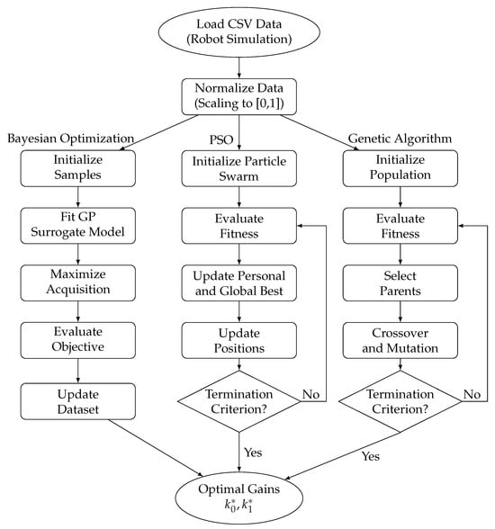
Figure 1.
Workflow illustrating Bayesian Optimization (left), Particle Swarm Optimization (center), and Genetic Algorithm (right) for obtaining the optimal control gains and .
2.5. Load CSV Data
The data loading stage was implemented in Python version 3.8.1 using the pandas and numpy libraries [13,14]. The script to load data in .py file performs the following operations:
- CSV Import. As mentioned before, four CSV files are loaded: k0.csv and k1.csv that contain the controller gain vectors (14) and (10) explored in the parameter sweep, each of dimension ; and Z1.csv and Z2.csv that contain the time-series NN tracking errors (7) per simulation, each of dimension . These files are imported as NumPy arrays using pd.read_csv(filename, header=None).values.
- Dimensionality Checks. This is performed to ensure consistency and to guarantee that each gain combination has a corresponding tracking error trajectory. Then, the script validates
- Computation of Steady-State Errors. To condense the time series into a scalar measure of control performance per axis, for each simulation, the final NN tracking error is summarized as the mean absolute error over the last 100 samples as
- Cost Function Computation. The cost per simulation is defined as the sum of both steady-state errors:This represents the global tracking deviation for the given gains (18).
- Feature Matrix Assembly. A matrix is constructed by stacking the gain vectors (18):This matrix serves as the input space for subsequent optimization algorithms.
This modular approach separates the dataset preprocessing logic from the optimization routines and ensures reproducibility of the feature-target mapping. By returning the tuple , the pipeline retains access to both the summarized metrics and the full error trajectories for visualization or additional analysis.
2.6. Normalize Data
To prevent variables with larger numerical ranges from dominating the search process, a normalization procedure is applied. This is performed after loading the CSV data to rescale all input variables into a common range, typically [0, 1]. Also, this procedure improves the performance and convergence speed of optimization algorithms such as BO, PSO, and GA [15,16,17].
The data normalization procedure was implemented in Python using scikit-learn and joblib [18]. The script to normalize data in .py processes the gains and cost function to improve convergence stability across the optimization methods. The workflow includes the following steps:
- Gain Normalization. To ensure that each gain dimension contributes equally to the surrogate model, the matrix (23) that has the controller gains and is rescaled to the unit hypercube . This operation is performed by using the following transformation: where and are vectors containing the minimum and maximum of each column, respectively.
- Cost Function Normalization. To prevent numerical scaling issues when fitting surrogate models or computing particle and genetic algorithm fitness scores, the scalar cost values (22), which represent the aggregate steady-state tracking error per simulation, are normalized using the same approach as the following:
- Persistence of Scaling Parameters. The fitted scalers (scaler_k.pkl and scaler_J.pkl) are saved to disk using joblib.dump. This allows the optimization .py files to apply the same transformation to new candidate gains during optimization and to inverse-transform normalized results back to the original gain space as follows:
- Verification. To confirm numerical consistency, after normalization and descaling, the .py file asserts the following:
This normalization procedure ensures that BO, PSO, and GA algorithms operate in a uniform and reproducible numerical domain, thus improving convergence reliability. The normalized controller gains are represented as the vector
where each component is obtained by applying the normalization transformation to the original gains and defined in (18).
Also, the normalized tracking errors are defined as
where represents the original tracking errors for joint i, and are the global minimum and maximum over all elements of , with j indexing the simulation number (corresponding to a specific pair), and k indexing the discrete-time steps within the simulation. This normalization rescales the full time series data to the interval , ensuring stability and comparability across evaluations.
The mapping of the gain vector (25) and the normalized matrices and (26) allows the optimization process to explore the search space consistently while maintaining the ability to recover the original gains and tracking errors using the inverse transformation. Consequently, the normalized parameters and matrices and serve as the inputs for all subsequent optimization algorithms BO, PSO, and GA, and their optimal values can later be projected back to the control parameter space of the 2-DOF robotic manipulator represented in dicrete time (4).
2.7. Bayesian Optimization Algorithm
The BO branch constitutes a sequential search procedure for minimizing the combined tracking error of the neural discrete-time sliding mode controller applied to the 2-DOF robot manipulator. This procedure relies on a surrogate probabilistic model and iteratively refines the estimation of the optimal control gains . The implementation leverages the scikit-optimize library in Python [19]. Each step of the workflow in the left part of Figure 1 is detailed as follows:
- Fit Gaussian Process (GP) Surrogate Model. In this work, two independent Gaussian Process Regressors (GaussianProcessRegressor) are trained to model the normalized tracking errors and , which are defined as follows:where are vectors of length 5000 time steps per simulation. The kernel hyperparameters are optimized by maximizing the marginal likelihood, and the resulting models provide predictive means and variances.These outputs correspond to the normalized cost values and derived from the steady-state tracking errors described in (24) in Section 2.6.
- Maximize Acquisition Function. To select the next candidate, the expected improvement criterion is optimized over the input space . The objective function for BO combines both tracking errors as follows:where denotes the GP prediction where the default optimizer in scikit-optimize is employed in the expected improvement maximization.
- Evaluate Objective. Now, using the surrogate models, the selected normalized gains are denormalized to the original scale of and evaluated by predicting and of (27). This denormalization process uses the inverse transformation , where are the normalized gain values for the original gains (14) and (10) obatained in Section 2.6.
- Update Dataset. After selecting a new gain configuration , the associated cost is computed either through the surrogate model or via a direct simulation. Then, following the evaluation of the new gain configuration, the resulting data point is integrated into the training set. This updated dataset is used to retrain the Gaussian Process model, thereby enhancing its predictive performance across the cost landscape associated with the discrete-time sliding mode controller (8) that governs the motion of the 2-DOF planar robot in discrete time (4) via the recurrent high-order NN (6).
- Optimal Gains. At this point, until the improvement in the cost function falls below a threshold, the optimization loop is repeated for iterations. At the end of this process, the best performing normalized parameters are transformed back into the original gain space using the inverse normalization function. These Optimal Gains correspond to the optimal tuning of the discrete-time sliding mode controller, minimizing the aggregate tracking error J (22) computed from the steady-state values of and of (7) (or in case and of (21)), the time-domain tracking errors for each joint.
2.8. Particle Swarm Optimization Algorithm
The PSO branch draws inspiration from the emergent collective behavior of biological swarms such as bird flocks or fish schools [21]. Within the goal of this project, PSO is applied as a population-based metaheuristic algorithm designed to minimize the aggregate tracking error J (22) of the neural discrete-time sliding mode controller (8) implemented on the 2-DOF robotic manipulator in discrete time (4).
The optimization presented in this work is carried out over the normalized gain space , where each particle in the swarm represents the normalized gains (25). These gains, as candidate solutions, are mapped to the original controller parameters (18) with a step of two by inverse normalization for performance evaluation using the NN tracking error metrics derived from and , as defined in (7) (or the original tracking errors and of (21)). This is due to the recurrent high-order NN (5) reproducing the behavior of the 2-DOF robotic manipulator in discrete time (4).
The PSO optimization process follows the central workflow depicted in Figure 1 and is implemented using the scikit-optimize and pyswarm libraries. The algorithm simulates a swarm of particles moving in the gain space, each adjusting its velocity based on both its personal best performance and the best performance of the swarm as a whole. This collaborative mechanism allows the swarm to efficiently explore the cost landscape and converge to the global minimum.
The main steps of the PSO procedure are detailed below.
- Initialize Particle Swarm. To begin the optimization process, a swarm of particles is initialized within the normalized gain space , as defined in Section 2.6. Each particle i is assigned an initial position vector , representing a candidate normalized gain vector (25) and an initial velocity vector . The velocity components are randomly sampled from a uniform distribution in the interval , which allows for exploratory movement within the search space at the start of the algorithm.
- Evaluate Fitness. For each particle position , representing a candidate normalized gain vector as defined in (25), the fitness function is computed using the surrogate models. Specifically, the predicted tracking cost is calculated aswhere and are the outputs of the Gaussian Process regressors trained on the normalized dataset, representing approximations of the normalized cost function (24) derived from normalized tracking error matrices and as defined in (26).
- Update Personal and Global Best. Each particle maintains its personal best position , and the swarm identifies the global best position g based on the fitness function as follows:The fitness function is evaluated using the surrogate-based approximation defined in (28). Note: Although Equation (28) was originally introduced in the context BO, it remains valid for the PSO procedure, since the same Gaussian Process surrogate models are used to estimate the normalized tracking errors and based on the steady-state values derived from and (26) as described in Section 2.6.
- Update Positions. Each particle updates its velocity and moves to a new location in the normalized gain space . First, the velocity is updated according to the standard PSO update rule: where is the inertia weight that controls the influence of the previous velocity; are the cognitive and social acceleration coefficients; are vectors of uniformly distributed random numbers that introduce stochasticity in exploration. Then, the particle’s position is updated as and clipped to remain within the bounds of the normalized domain:This ensures that each particle remains within the feasible search region for the normalized gains (25).
- Termination Criterion. The PSO algorithm proceeds iteratively until one of the following stopping conditions is met:
- –
- the number of iterations reaches a predefined maximum of , or
- –
- the absolute improvement in the global best fitness value over consecutive iterations is smaller than a convergence threshold .
This condition is checked at each iteration. If satisfied (Yes), the loop terminates and proceeds to the final block (Optimal Gains). Otherwise (No), the algorithm returns to the Evaluate Fitness step to continue refining the swarm’s exploration of the normalized gain space .This convergence behavior ensures that the PSO process balances global exploration and local refinement while searching for the optimal normalized gains , which can then be inverse-transformed to obtain the corresponding gains for the controller. - Optimal Gains . Once the termination criterion is satisfied, the global best particle position is selected as the optimal solution in the normalized space. To recover the corresponding control gains for the discrete-time sliding mode controller, the inverse normalization transformation is applied using the scaler saved in Section 2.6:These gains represent the optimal tuning configuration that minimizes the aggregate tracking error defined by the surrogate-based fitness function , which itself is derived from the normalized steady-state tracking errors and described in (26).The resulting Optimal gains are the values alongside their corresponding cost J computed from the original tracking error matrices. This optimal pair can now be implemented in the neural discrete-time sliding mode controller (8) to achieve improved performance in joint trajectory tracking for the 2-DOF planar robot in discrete time (4).
2.9. Genetic Algorithm Optimization
The GA branch employs a population-based evolutionary method to minimize the overall steady-state tracking error of the neural discrete-time sliding mode controller for the 2-DOF planar robot. This is illustrated in the rightmost branch of the workflow in Figure 1 and is implemented using the DEAP [22] and scikit-optimize [23] libraries. The optimization operates within the normalized gain space , where each candidate solution represents a gain vector , as defined in (25). These are obtained by scaling the original gain set (see (18)), as discussed in Section 2.6.
The GA procedure comprises the following stages:
- Initialize Population. A starting population of individuals is generated by random sampling from the normalized domain . Each individual represents a potential controller gain vector. Uniform initialization is applied to guarantee broad exploration of the search space and maintain genetic diversity for the evolutionary algorithm.
- Evaluate Fitness. Each individual’s fitness is assessed through the Gaussian Process (GP) surrogate model. The fitness function combines predicted normalized tracking costs aswhere and are predictions from GP models trained on the normalized error matrices and (see (26)). This cost function aligns with (28) from the Bayesian Optimization framework and remains applicable here, as identical surrogate models are employed.
- Select Parents. A tournament selection mechanism is used with a tournament size of . In this process, random groups of individuals are created from the population, and the highest-fitness candidate from each group is chosen for reproduction. This approach maintains an effective equilibrium between selecting high-performing solutions and sustaining population diversity.
- Crossover and Mutation. The next generation is produced through the following:
- –
- Crossover. Simulated Binary Crossover (SBX) [24,25] is performed with crossover probability . For parent solutions, offspring are generated viawhere the distribution index determines offspring diversity.
- –
- Mutation. Polynomial mutation operates with probability , adding controlled random variations:with solutions constrained to the normalized space .
- Termination Criterion. The optimization runs for up to generations or stops earlier if the relative improvement in the best fitness value drops below . Each iteration checks the stopping condition: if it is not satisfied (No), the process returns to the fitness evaluation; if satisfied (Yes), the algorithm ends and proceeds to the Optimal Gains block.
- Optimal Gains . Upon convergence, the optimal normalized solution is identified. The actual controller gains are obtained by reversing the normalization:producing the final control parameters. These optimized gains minimize the surrogate-based cost function that represents the robot joints’ steady-state tracking errors.
3. Results
To enhance the transparency of the optimization process, progression plots are provided for each algorithm: BO (Figure 2), PSO (Figure 3), and GA (Figure 4). Each figure is arranged as a 2 × 3 grid: the top row shows Joint 1 and the bottom row Joint 2; the columns correspond to early, mid, and final stages of the search. In every panel, the black curve is the reference, the blue curve is the estimated position , and the red curve (right axis) is the estimation error . These signals are reconstructed directly from the dataset using and . When available, the three milestones are taken from the optimization logs at iterations 1, 25, and 50; otherwise, a representative early/mid/final triplet is selected by sorting the per-simulation cost and picking worst/median/best. This presentation complements the convergence summary (Figure 5) by showing how tracking quality improves over time in each method.
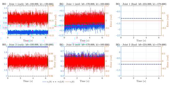
Figure 2.
Progression of BO. Columns depict early, mid, and final stages (either iterations 1/25/50 from the log or worst/median/best by J). Top: Joint 1; bottom: Joint 2. Black: reference; blue: estimated position ; red (right axis): estimation error . A clear reduction in steady-state error from early to final is observed, with BO retaining some exploratory behavior in the mid stage before settling, consistent with its acquisition-driven search and the global trend shown in Figure 5. Left axis in rad; right axis in rad for Joint 1 and rad/s for Joint 2.
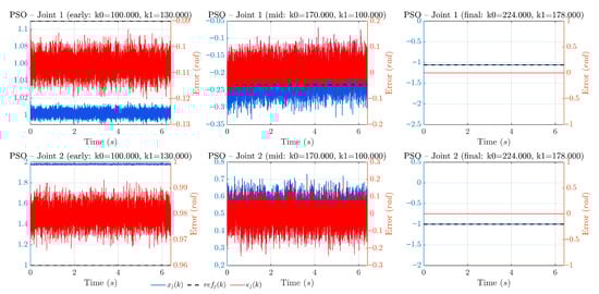
Figure 3.
Progression of PSO. From early to mid, the swarm quickly drives the trajectories closer to the references, and the final stage shows small tracking errors with minor residual transients. This fast improvement mirrors the rapid convergence behavior reported in Figure 5. Axis conventions as in Figure 2.
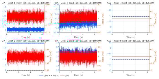
Figure 4.
Progression of GA. The early stage exhibits larger errors, which decrease steadily by the mid stage as selection, crossover, and mutation refine the population; the final stage presents low steady-state errors comparable to the best configurations. This gradual improvement aligns with the generation-wise convergence trend in Figure 5. Axis conventions as in Figure 2.
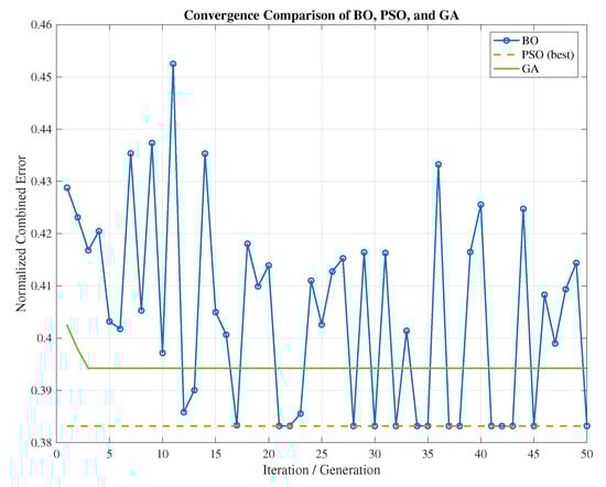
Figure 5.
Convergence comparison of BO, PSO, and GA.
3.1. Dataset Neural Sliding Mode Control Simulation
As a result of the script and for the dataset obtained in Section 2.4, Figure 6 and Figure 7 show simulation comparisons for all tracking performance of the proposed control scheme for the 2-DOF planar robotic manipulator for Joints 1 and 2. Each figure displays the reference signal (in black), the real joint position (in red), and the estimated position provided by recurrent high-order NN (in blue) for all simulations with the 6400 different controller gain values and (18).
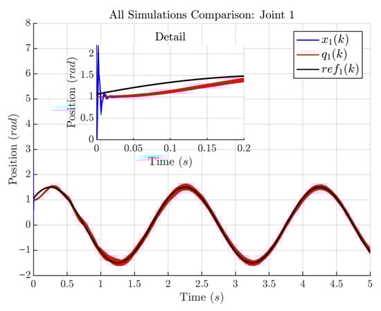
Figure 6.
Tracking performance for Joint 1. The reference trajectory is shown in black, the measured position in red, and the estimated state in blue. A zoomed-in region illustrates the tracking precision at the beginning of the simulation.
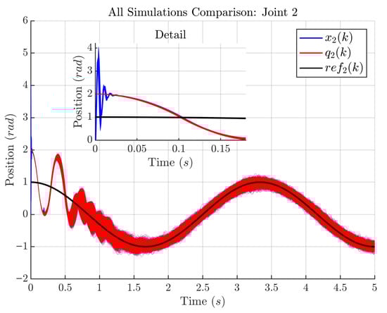
Figure 7.
Tracking performance for Joint 2. Black: ; red: measured ; blue: estimated . Semi-transparent overlays depict 6400 simulations across the gain space. The inset zoom highlights the initial transient.
In Figure 6, the measured position and the estimated state closely follow reference over the full 5 s simulation. The red and blue semi-transparent traces correspond to simulations with different controller gains, allowing visual assessment of variability; the narrow dispersion indicates consistent tracking. The inset zoom emphasizes the initial transient. These results also show that the recurrent high-order NN accurately estimates the robot state, as matches with high fidelity.
Figure 7 shows analogous results for Joint 2. After a short transient, both and align with , demonstrating robust tracking over the full sweep of gains. The agreement between and further validates the effectiveness of the neural estimator. To explicitly illustrate optimization progress (beyond aggregate tracking), it includes per-algorithm progression plots (early/mid/final milestones taken from iterations 1, 25, and 50 or a worst/median/best fallback), see Figure 2, Figure 3 and Figure 4, and the convergence of the objective value over iterations/generations in Figure 5. These plots complement Figure 6 and Figure 7 by showing how performance improves as each method converges.
Table 1 reports the mean values of the state estimation errors for clarity. MAE (mean absolute error) is used as the primary metric and also the mean error (bias) and RMSE (root mean squared error) are reported. For the joint positions, rad and rad for and , respectively, are obtained with very small mean errors ( rad and rad), indicating negligible bias. The corresponding RMSE values ( rad and rad) are close to the MAE, suggesting the absence of large outliers in the position estimates. For the joint velocities, the MAE is rad/s for and rad/s for , with mean errors rad/s and rad/s, respectively. The larger gap between RMSE and MAE for ( vs. rad/s) points to sporadic higher deviations in the velocity estimate of Joint 2. Table 1 complements Figure 6 and Figure 7 and clearly demonstrates the accuracy of the state estimation algorithm.

Table 1.
Mean values of the state estimation errors (MAE as the primary clarity metric).
3.2. Optimal Control Gains for BO, PSO, and GA
Table 2, Table 3, Table 4 and Table 5 summarize the performance of the optimization algorithms applied to the tuning of the neural discrete-time sliding mode controller gains for the robot manipulator.
Table 2.
Optimal gains and average steady-state tracking errors.
Table 3.
Computational time per process.
Table 4.
Number of evaluations per algorithm.
Table 5.
Model precision (R2).
Table 2 and Table 3 jointly summarize accuracy and efficiency under an identical pipeline (shared data loading/normalization and a single Python implementation). The optimal gains concentrate in a narrow region (, ), and the average steady-state errors are computed over the final 0.1 s ( s). Quantitatively, PSO attains the lowest error in Joint 1 ( rad), GA the lowest in Joint 2 ( rad), and BO remains competitive in both ( rad; rad) while using only 50 evaluations. In terms of time, PSO is the fastest (23.44 s), BO is similar (23.65 s), and GA is costlier (61.98 + 7.70 s refinement s), consistent with its larger evaluation budget.
Table 4 shows that the GA requires the highest number of function evaluations (7500), significantly more than PSO with 1500 and BO with only 50. This extensive sampling by GA likely contributes to its ability to find a more refined solution, as reported in Table 2, but comes at the cost of considerably increased computational time.
Table 5 presents the predictive accuracy of the Gaussian Process surrogate models used in the optimization, reported through the coefficient of determination . The low values for both joints (0.0336 for DOF1 and 0.0084 for DOF2) indicate that the surrogate models provide only coarse approximations of the true cost landscape. As such, while they offer a useful heuristic for guiding the search process, direct simulation evaluations remain essential to ensure accurate assessment of candidate solutions.
Figure 5 illustrates the convergence behavior of the three optimization algorithms over 50 iterations or generations. The BO trajectory shows significant oscillations, reflecting its probabilistic sampling strategy and active exploration of the gain space. In contrast, both PSO and GA exhibit rapid convergence within the first few iterations, stabilizing early in low-error regions. For PSO and GA, the plot displays the best normalized cost value found at each generation, highlighting their exploitation-driven search dynamics. The dashed horizontal line representing PSO marks the lowest final cost among the three methods, consistent with the results reported in Table 2. These convergence profiles illustrate the distinct exploration–exploitation balances intrinsic to each optimization strategy. For clarity, Figure 5 plots the normalized objective (built from the steady-state tracking-error cost defined in Section 2.6; lower is better). Each curve reports the best-so-far value as a function of iteration/generation t, and all methods are run with an equal budget of 50 iterations/generations. The y-axis is unitless due to normalization to , and the x-axis counts iterations (BO) or generations (PSO/GA).
The early stagnation of the PSO curve suggests that the swarm quickly located a promising region in the search space and collectively converged without further significant improvement, possibly due to limited diversity or suboptimal balance in its exploration parameters. On the other hand, the persistent oscillations in the BO curve indicate that the acquisition function continues to propose exploratory samples far from previously evaluated regions. This reflects the BO strategy’s emphasis on global search, even after identifying near-optimal regions, which may delay convergence but can help avoid premature local optima. Such behavior highlights that while BO may take longer to settle, it remains valuable in problems where the cost landscape is highly multimodal or where evaluations are costly and limited in number.
Overall, the results demonstrate that all three optimization strategies effectively identify high-performance gain configurations. BO offers a favorable trade-off between tracking performance and computational efficiency, whereas the GA achieves the lowest tracking cost at the expense of significantly higher computational effort and number of evaluations.
Figure 8 shows the torques produced over a 5 s simulation with ms. Dashed horizontal lines indicate actuator limits: Nm for Joint 1 and Nm for Joint 2. Both and remain within their bounds, exhibiting the expected behavior of SMC while satisfying the torque requirements stated in Section 2.3. The apparent saturation in the control signals is an intended consequence of the control law in (8). Whenever , the second branch is activated and the commanded torque is clipped to with the sign of . This explains the plateaus at Nm (Joint 1) and Nm (Joint 2), ensures compliance with actuator limits, and produces the characteristic behavior typical of SMC.
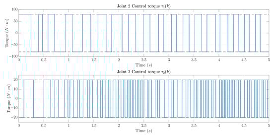
Figure 8.
PSO–tuned discrete-time SMC: control torques ((top) , (bottom) ).
4. Discussion
The results presented in Section 3 confirm the effectiveness of the proposed AI-based optimization framework for tuning the gains of a neural discrete-time sliding mode controller applied to a 2-DOF robotic manipulator. However, several additional aspects merit discussion to contextualize the contributions and limitations of this work.
First, while this study focused on three popular metaheuristic algorithms—Bayesian Optimization (BO), Particle Swarm Optimization (PSO), and Genetic Algorithms (GAs)—it is important to note that other AI-driven and classical optimization techniques are available. Alternatives such as Differential Evolution, Ant Colony Optimization, Reinforcement Learning-based controllers, or even gradient-based deterministic methods (e.g., Sequential Quadratic Programming) could also be explored. Each approach brings trade-offs in terms of convergence rate, robustness, and computational demand, which may prove beneficial in different application scenarios.
Second, the optimization objective in this study targeted the minimization of the steady-state tracking error, as defined by the cost function in (22). While this metric is fundamental for ensuring accurate long-term tracking, it does not explicitly account for transient dynamics such as overshoot, settling time, or control energy expenditure.
Third, the simulation data used for training the surrogate models and evaluating the controller was generated through a systematic sweep of normalized gain values. Despite the limited size of the dataset (on the order of hundreds of samples), the convergence of BO, PSO, and GA to similar optimal regions indicates that the data were sufficiently informative to guide the optimization processes. This also highlights the advantage of working in a normalized gain space, which allowed the models to generalize well across the explored domain.
It is also worth noting that the surrogate models used in BO and PSO approximated the cost landscape with relatively low precision (as reflected by the scores in Table 5). Nevertheless, the optimization routines remained effective due to the reinforcement provided by direct simulation evaluations. This suggests that even modest-quality models can support efficient gain tuning when combined with simulation-based corrections.
Finally, although the neural plant model employed an EKF for online adaptation of covariance matrices, future research could investigate other adaptive training mechanisms such as recursive least squares, ensemble learning, or deep learning-based dynamics estimators. Incorporating uncertainty quantification into the plant model could further improve the robustness of the control strategy in real-world settings.
In summary, the methodology proposed in this study establishes a solid foundation for AI-based controller optimization. It remains extensible to other objective functions, optimization techniques, and controller architectures, thereby offering a flexible framework for advancing autonomous control of robotic systems.
Recent studies have explored data-driven or metaheuristic tuning of robust controllers in robotic applications. For instance, work [26] combines SMC with online BO for a bio-inspired underwater robot, showing marked improvements in depth and pitch regulation after roughly fifty online updates while maintaining Lyapunov-stable operation. In terrestrial settings, local BO with crash constraints has been proposed to tune controller parameters under hardware limits safely [27]. Within metaheuristics, work [28] integrates PSO with a modified power–rate SMC to mitigate chattering and simplify tuning on a multi-DOF manipulator with experimental validation; the authors in [29] compare several metaheuristics (DE, PSO, hybrids) for manipulator trajectory tracking using a multi-term objective (position/orientation/joint errors) and uniform iteration budgets; and in Keshti [30] employ GA to tune SMC gains for human-arm trajectory tracking, focusing on minimizing summary tracking error.
Compared with the above, we explicitly adopt a discrete-time SMC and a recurrent high-order neural network NN that reproduces the dynamics of the 2-DOF manipulator (serving as the predictive plant for indirect control). Within this discrete-time setting, we evaluate the same controller and dataset across BO, PSO, and GA, enabling a direct trade-off reading between accuracy and computation (Table 2 and Table 3). Table 2 shows that PSO attains the lowest steady-state error for Joint 1, while GA attains the lowest for Joint 2 (by a narrow margin), and BO is competitive in both joints. From Table 3, PSO achieves the shortest optimization time among the three, BO is similar, and GA is noticeably more expensive—consistent with prior reports that PSO offers fast convergence for nonlinear objectives [28] and that BO is attractive for sample-efficient tuning [26,27]. Together with the progression plots and convergence curves, these results contextualize our contribution: a reproducible, apples-to-apples benchmark of discrete-time SMC gain tuning with a recurrent high order NN-based plant model for a 2-DOF robot, revealing that PSO is an excellent first choice when compute is tight, BO is attractive when safe, sample-efficient exploration is needed, and GA can yield competitive accuracy at higher computational cost. Table 6 shows the mentioned comparison.
Table 6.
Comparison with related works on data-driven/metaheuristic controller tuning.
Following industry practice, steady state is declared once the trajectory enters and remains within a tolerance band for a dwell time. In accordance with ISO 9283 [31] “position stabilization time,” the band can be tied to robot repeatability or set as a percentage band (e.g., ), and the dwell time ensures persistence inside the band. In our experiments (sampling at 1 kHz), we adopt a 0.1 s dwell (100 samples) once the band is entered, and compute steady-state errors over that dwell segment. This aligns with the classical settling-time definition based on tolerance bands used in control theory [32].
5. Conclusions
This work presented a comprehensive AI-based optimization framework for tuning the gains of a neural discrete-time sliding mode controller applied to a two-degree-of-freedom robotic manipulator. The controller was indirectly implemented through a neural network trained with an EKF, allowing the estimation of the plant dynamics and facilitating robust control under model uncertainties.
Three optimization strategies—Bayesian Optimization (BO), Particle Swarm Optimization (PSO), and Genetic Algorithms (GAs)—were evaluated using a normalized parameter space and surrogate modeling based on Gaussian Processes. The optimization process was driven by the minimization of normalized steady-state tracking errors for both joints of the robot. The normalization framework enabled a unified treatment of the gain space and tracking error costs, improving convergence efficiency and reproducibility.
The results demonstrated that all three metaheuristics successfully identified high-performance gain configurations. GAs achieved the lowest tracking cost but at the expense of a significantly higher number of evaluations and computation time. BO and PSO yielded nearly identical results with much lower computational effort. These findings highlight that the proposed methodology provides a flexible and efficient solution for automatic controller tuning, especially in scenarios where analytical models are unavailable or costly to evaluate.
Future work will explore real-time adaptation of controller gains using online learning techniques and extend the optimization framework to multi-objective formulations involving control effort, energy consumption, and robustness metrics.
Funding
This work was supported by Universidad de Guadalajara through the Programa de Apoyo a la Mejora en las Condiciones de Producción de las Personas Integrantes del SNII y SNCA, (PROSNII), 2025.
Institutional Review Board Statement
Not applicable.
Informed Consent Statement
Not applicable.
Data Availability Statement
No new data were created or analyzed in this study. Data sharing is not applicable to this article.
Acknowledgments
The author gratefully acknowledges the invaluable support provided by the Universidad de Guadalajara, Centro Universitario de los Lagos.
Conflicts of Interest
The author declares no conflicts of interest.
Abbreviations
The following abbreviations are used in this manuscript:
| AI | Artificial Intelligence |
| BO | Bayesian Optimization |
| EKF | Extended Kalman Filter |
| GA | Genetic Algorithms |
| GP | Gaussian Process |
| NN | Neural Network |
| PSO | Particle Swarm Optimization |
| SMC | Sliding Mode Control |
| 2-DOF | Two-Degree-Of-Freedom |
References
- Silaa, M.Y.; Barambones, O.; Bencherif, A. Robust adaptive sliding mode control using stochastic gradient descent for robot arm manipulator trajectory tracking. Electronics 2024, 13, 3903. [Google Scholar] [CrossRef]
- Sosa Méndez, D.; Bedolla-Martínez, D.; Saad, M.; Kali, Y.; García Cena, C.E.; Álvarez, Á.L. Upper-limb robotic rehabilitation: Online sliding mode controller gain tuning using particle swarm optimization. Robotics 2025, 14, 51. [Google Scholar] [CrossRef]
- Wang, Q.; Liu, D.; Carmichael, M.G.; Aldini, S.; Lin, C.T. Computational model of robot trust in human co-worker for physical human-robot collaboration. IEEE Robot. Autom. Lett. 2022, 7, 3146–3153. [Google Scholar] [CrossRef]
- Martinez-Cantin, R. Bayesian optimization with adaptive kernels for robot control. In Proceedings of the 2017 IEEE International Conference on Robotics and Automation (ICRA), Singapore, 29 May–3 June 2017; pp. 3350–3356. [Google Scholar]
- Saidi, K.; Bournediene, A.; Boubekeur, D. Genetic Algorithm Optimization of sliding Mode Controller Parameters for Robot Manipulator. Int. J. Emerg. Technol. 2021, 12, 119–127. [Google Scholar]
- Lima, G.d.S.; Porto, D.R.; de Oliveira, A.J.; Bessa, W.M. Intelligent control of a single-link flexible manipulator using sliding modes and artificial neural networks. Electron. Lett. 2021, 57, 869–872. [Google Scholar] [CrossRef]
- Mosharafian, S.; Afzali, S.; Bao, Y.; Velni, J.M. A deep reinforcement learning-based sliding mode control design for partially-known nonlinear systems. In Proceedings of the 2022 European Control Conference (ECC), London, UK, 12–15 July 2022; pp. 2241–2246. [Google Scholar]
- Duan, X.; Liu, X.; Ma, Z.; Huang, P. Sampled-Data Admittance-Based Control for Physical Human–Robot Interaction With Data-Driven Moving Horizon Velocity Estimation. IEEE Trans. Ind. Electron. 2024, 72, 6317–6328. [Google Scholar] [CrossRef]
- Spong, M.W.; Hutchinson, S.; Vidyasagar, M. Robot Modeling and Control; John Wiley & Sons: Hoboken, NJ, USA, 2006. [Google Scholar]
- Pizarro-Lerma, A.; García-Hernández, R.; Santibáñez, V. Fine-tuning of a fuzzy computed-torque control for a 2-DOF robot via genetic algorithms. IFAC- PapersOnLine 2018, 51, 326–331. [Google Scholar] [CrossRef]
- Kazantzis, N.; Kravaris, C. Time-discretization of nonlinear control systems via Taylor methods. Comput. Chem. Eng. 1999, 23, 763–784. [Google Scholar] [CrossRef]
- Castañeda, C.E.; Esquivel, P. Decentralized neural identifier and control for nonlinear systems based on extended Kalman filter. Neural Netw. 2012, 31, 81–87. [Google Scholar] [CrossRef]
- Siebert, J.; Groß, J.; Schroth, C. A systematic review of python packages for time series analysis. arXiv 2021, arXiv:2104.07406. [Google Scholar] [CrossRef]
- Rayhan, R.; Rayhan, A.; Kinzler, R. Exploring the Power of Data Manipulation and Analysis: A Comprehensive Study of NumPy, SciPy, and Pandas. 2023. Available online: https://www.researchgate.net/publication/373217405_Exploring_the_Power_of_Data_Manipulation_and_Analysis_A_Comprehensive_Study_of_NumPy_SciPy_and_Pandas (accessed on 14 September 2025). [CrossRef]
- Pedregosa, F.; Varoquaux, G.; Gramfort, A.; Michel, V.; Thirion, B.; Grisel, O.; Blondel, M.; Prettenhofer, P.; Weiss, R.; Dubourg, V.; et al. Scikit-learn: Machine learning in Python. J. Mach. Learn. Res. 2011, 12, 2825–2830. [Google Scholar]
- Liu, Z.; Zhao, K.; Liu, X.; Xu, H. Design and optimization of haze prediction model based on particle swarm optimization algorithm and graphics processor. Sci. Rep. 2024, 14, 9650. [Google Scholar] [CrossRef] [PubMed]
- Kim, Y.S.; Kim, M.K.; Fu, N.; Liu, J.; Wang, J.; Srebric, J. Investigating the impact of data normalization methods on predicting electricity consumption in a building using different artificial neural network models. Sustain. Cities Soc. 2025, 118, 105570. [Google Scholar] [CrossRef]
- Jolly, K. Machine Learning with Scikit-Learn Quick Start Guide: Classification, Regression, and Clustering Techniques in Python; Packt Publishing Ltd.: Birmingham, UK, 2018. [Google Scholar]
- Head, T.; Cherti, M.; Pedregosa, F.; Zhdanov, M.; Louppe, G.; Raffel, C.; Mueller, A.; Fauchere, N.; McInnes, L.; Grisel, O. Scikit-Optimize: Sequential Model-Based Optimization with Scikit-Learn. 2018. Available online: https://scikit-optimize.github.io/stable/ (accessed on 14 September 2025).
- Greif, L.; Hübschle, N.; Kimmig, A.; Kreuzwieser, S.; Martenne, A.; Ovtcharova, J. Structured sampling strategies in Bayesian optimization: Evaluation in mathematical and real-world scenarios. J. Intell. Manuf. 2025, 1–31. [Google Scholar] [CrossRef]
- Gad, A.G. Particle swarm optimization algorithm and its applications: A systematic review. Arch. Comput. Methods Eng. 2022, 29, 2531–2561. [Google Scholar] [CrossRef]
- Malashin, I.; Masich, I.; Tynchenko, V.; Nelyub, V.; Borodulin, A.; Gantimurov, A. Application of natural language processing and genetic algorithm to fine-tune hyperparameters of classifiers for economic activities analysis. Big Data Cogn. Comput. 2024, 8, 68. [Google Scholar] [CrossRef]
- Hackeling, G. Mastering Machine Learning with Scikit-Learn; Packt Publishing Ltd.: Birmingham, UK, 2017. [Google Scholar]
- Roeva, O.; Zoteva, D.; Roeva, G.; Ignatova, M.; Lyubenova, V. An Effective Hybrid Metaheuristic Approach Based on the Genetic Algorithm. Mathematics 2024, 12, 3815. [Google Scholar] [CrossRef]
- Fanggidae, A.; Prasetyo, M.C.; Polly, Y.T.; Boru, M. New Approach of Self-Adaptive Simulated Binary Crossover-Elitism in Genetic Algorithms for Numerical Function Optimization. Int. J. Intell. Syst. Appl. Eng. 2024, 12, 174–183. [Google Scholar]
- Hamamatsu, Y.; Rebane, J.; Kruusmaa, M.; Ristolainen, A. Bayesian Optimization Based Self-Improving Sliding Mode Controller For a Bio-Inspired Marine Robot. In Proceedings of the 2024 IEEE/OES Autonomous Underwater Vehicles Symposium (AUV), Boston, MA, USA, 18–20 September 2024; pp. 1–6. [Google Scholar]
- von Rohr, A.; Stenger, D.; Scheurenberg, D.; Trimpe, S. Local Bayesian optimization for controller tuning with crash constraints. at-Automatisierungstechnik 2024, 72, 281–292. [Google Scholar] [CrossRef]
- Sinan, S.; Fareh, R.; Hamdan, S.; Saad, M.; Bettayeb, M. Modified power rate sliding mode control for robot manipulator based on particle swarm optimization. IAES Int. J. Robot. Autom. 2022, 11, 168. [Google Scholar] [CrossRef]
- Lopez-Franco, C.; Diaz, D.; Hernandez-Barragan, J.; Arana-Daniel, N.; Lopez-Franco, M. A metaheuristic optimization approach for trajectory tracking of robot manipulators. Mathematics 2022, 10, 1051. [Google Scholar] [CrossRef]
- Kheshti, M.; Tavakolpour-Saleh, A.; Razavi-Far, R.; Zarei, J.; Saif, M. Genetic Algorithm-Based Sliding Mode Control of a Human Arm Model. IFAC-PapersOnLine 2022, 55, 2968–2973. [Google Scholar] [CrossRef]
- ISO 9283:1998; Manipulating Industrial Robots—Performance Criteria and Related Test Methods; Technical Report. ISO: Geneva, Switzerland, 1998.
- Nise, N.S. Control Systems Engineering; John Wiley & Sons: Hoboken, NJ, USA, 2019. [Google Scholar]
Disclaimer/Publisher’s Note: The statements, opinions and data contained in all publications are solely those of the individual author(s) and contributor(s) and not of MDPI and/or the editor(s). MDPI and/or the editor(s) disclaim responsibility for any injury to people or property resulting from any ideas, methods, instructions or products referred to in the content. |
© 2025 by the author. Licensee MDPI, Basel, Switzerland. This article is an open access article distributed under the terms and conditions of the Creative Commons Attribution (CC BY) license (https://creativecommons.org/licenses/by/4.0/).