Digital Twin Driven Four-Dimensional Path Planning of Collaborative Robots for Assembly Tasks in Industry 5.0

Abstract

Collaborative robots are vital in Industry 5.0 operations. They are utilized to perform tasks in collaboration with humans or other robots to increase overall production efficiency and execute complex tasks. Aiming at a comprehensive approach to assembly processes and highlighting new applications of collaborative robots, this paper presents the development of a digital twin (DT) for the design, monitoring, optimization and simulation of robots’ deployment in assembly cells. The DT integrates information from both the physical and virtual worlds to design the trajectory of collaborative robots. The physical information about the industrial environment is replicated within the DT in a computationally efficient way that aligns with the requirements of the path planning algorithm and the DT’s objectives. An enhanced artificial fish swarm algorithm (AFSA) is utilized for the 4D path planning optimization, taking into account dynamic and static obstacles. Finally, the proposed framework is utilized for the examination of a case in which four industrial robotic arms are collaborating for the assembly of an industrial component.

1. Introduction

Industry 5.0 comprises the subsequent phase of industrial evolution following Industry 4.0 [1]. Industry 5.0 incorporates sustainability and resilience in an anthropocentric way to create value from the production systems [2]. Industry 5.0 transcends the traditional confines of automation and digitalization by emphasizing the development of collaborative systems between humans and machines [3]. This is achieved through the collaboration between human skills and advances in technology, personalized and flexible production, and increased overall efficiency and decision-making in real time [4]. The innovations of Industry 5.0 are feasible through the solutions offered by modern technologies, including artificial intelligence [5], cloud computing [6], collaborative robots [7], digital twins [8] and the Internet of Things [9].

Traditional industrial robots are particularly effective for executing tasks associated with operations on production lines. Collaborative robots are designed to work in the same environments as humans and robots to complete the assigned tasks [10,11]. Collaborative robots are equipped with sensors and the ability to react in unpredictable situations. These allow them to stop immediately when they detect unexpected obstacles in their path. Thus, they are particularly reliable and safe for performing tasks in changing environments [12]. Customer demand for customized items has been increased and industries are required to adapt from mass production models to smaller item packs and a broader variety of products. Traditional industrial robots have difficulty responding to production systems that require flexibility and constant reconfiguration [13].

Research on collaborative robots can include several areas, such as control algorithms, sensor integration and operation, and the design of human–robot interface systems [14]. The application of collaborative robots in the industrial environment requires the detailed definition of an overall framework from the problem analysis stage to the design and implementation of the solution [15]. The overall framework is created through a sequence of analysis and synthesis steps comprising the implementation conditions, the detailed description of the tasks, and the assignment of these tasks to the robots and humans involved [16].

In many existing industrial production processes, task allocation among collaborative robots is performed based on intuition or experiential knowledge [17]. This approach can lead to suboptimal performance, limited applications, and challenges in the optimization of the overall production system. Collaborative robots require more adaptive task allocation to accomplish the assigned tasks in real time. On the other hand, traditional industrial robots typically operate within a more rigid, predefined task assignment system. The coordinated interactions of multiple collaborative robots in a broader industrial system further increase the complexity and the importance of the task assignment. Thus, adjustments during the industrial processes are vital to ensure optimal production and adaptability to changing conditions.

The coordination of multiple collaborative robots leads to the formation of multi-robot systems that offer the ability to handle complex manufacturing processes. The multi-robot systems consist of several mobile or stationary robots equipped with sensing, computational, communication, and actuation functionalities, enabling them to collaboratively execute tasks in a decentralized manner [11]. The multi-robot system can execute tasks like assembly, painting, and object manipulation [11]. The coordination of collaborative robots in the assembly system requires efficient task planning [18].

Path planning is a fundamental concern in the field of robotics. It is defined as a sequence of points that determines the robot’s course from a starting to an ending location. There are several potential paths that can meet the above definition. Research on solving the path planning problem has focused on finding the shortest path. In the industrial environment several obstacles are encountered, the avoidance of collisions between robots and obstacles is ensured through the path planning process. While, for traditional robots, the path planning problem in cases like those described in references [19,20,21] has been extensively studied, due to the complex operation environment, research on collaborative robots’ path planning is limited.

A DT is a virtual representation of a physical system or an object characterized by real time bidirectional data flow to optimize the decision making process and the performance of its real-world counterpart [22]. The DTs create a virtual model that accurately replicates a physical system [23]. The virtual components are linked to their corresponding counterpart from the physical world. DT systems can use real-world data to simulate [24], monitor [25], and integrate virtual models such as artificial intelligence algorithms [26] to optimize the processes executed in the real-world system. They can be applied in several areas, such as power grids [27], agriculture [28], city management [29], and smart manufacturing [30]. DT technology offers new solutions in the industrial sector, particularly in areas where traditional approaches are limited, such as production system management [31] and factory design [30].

DTs can contribute to accomplishing the objectives set by Industry 5.0. They enable the optimization of decision making, maintenance scheduling, and monitoring the production conditions [32]. DTs analyze the physical system and its components through the dynamic and interactive assembly [33]. These systems can predict safety issues before they occur in the physical world and adapt the procedures in real time, ensuring safety in the industrial workspace [34]. DTs bridge the gap between digital tools and the physical world.

In manufacturing, DTs have been utilized to simulate and optimize assembly processes. Junnan et al. presented a hierarchical DT model for complicated assembly containing geometric and positioning constraints in relation to the physical layers [35]. Ma et al. proposed a DT approach to map the physical world digitally for quality control and optimization of complex assembly tasks [36]. Wang et al. combined transfer reinforcement learning with a DT system for task allocation in an assembly process where humans and robots cooperate [37]. Zhang et al. presented a DT framework for the assembly process of semi-automatic electronics when multiple changes happen [38]. Zhang et al. proposed a DT framework for the assembly of aircraft [39].

Du et al. simulated a robot’s trajectory in a DT and nominated an improved hybrid hierarchical bounding box collision detection algorithm for the detection of potential collisions during its execution [40]. Zhang et al. presented the use of DT in robotic machining tasks for large-scale components [41]. Xuan et al. utilized a DT for the simulation of a robot’s path generated by the A* algorithm [42]. Chen et al. presented the simulation of a 6 degree of freedom robotic arm in a virtual environment for accomplishing grasp tasks [43].

Despite DT technology being integrated into assembly and path planning solutions, there are several limitations in the existing literature. The utilization of a DT has been restricted to simulating the path of a single robot, thereby omitting the fundamental problems in the coexistence of multiple robots. These simulations are conducted in static environments where the positions of the obstacles are constant, which restricts their application to the dynamic environments of collaborative robots. Employing a DT only for replicating the path in a virtual environment neglects its full potential. This confined approach does not leverage the DT’s capabilities, such as real time data adaptation and predictive analytics. The inherent procedures of a DT, such as environmental modeling or data volume management, are not confronted for the path planning cases. Moreover, a research gap is identified in approaching the path planning of collaborative robots in assembly processes utilizing the capabilities offered by a DT. Studies on the application of a DT in assembly tasks frequently concentrate on individual procedures that occur during the assembly tasks, without considering their integration into an overall robotic workflow. As a result, the ability of the DT to provide end-to-end robotic assembly systems remains unexplored. The present literature reveals a research gap regarding the path planning of collaborative robots and the development of comprehensive DT systems for assembly processes. The aforementioned restrictions confine the applicability of existing research to the specification of Industry 5.0.

In this paper, the utilization of a DT is presented for assembly tasks with collaborative robots. In the DT, information from the physical world and assembly is gathered to find the optimal path of collaborative robots using a 4D path planning algorithm proposed in [44]. The DT is designed to be totally compatible with the 4D path algorithm, facilitating seamless information transmission across its operations. The virtual assets in the DT are created to simulate the behavior of their physical counterpart as accurately as possible. The DT model is optimized by removing unnecessary information to minimize the computational cost. Additionally, the presented model facilitates the management of the total production process and the available equipment. It accurately specifies the timing and duration of each robot’s implementation, thereby allowing its deployment across multiple tasks and reinforcing the flexibility and efficiency of the production process. Finally, a scenario involving four industrial robots with 6 degrees of freedom operating in the same environment for assembly tasks is examined.

The main contributions of the present paper can be summarized as follows:

• A DT framework is developed for simulating real-world industrial environments and achieving the path planning optimization of collaborative robots in assembly tasks;
• The DT is optimized for path planning of industrial robotic arms in the conditions of Industry 5.0;
• The integration of assembly information into the robot’s path planning;
• The management of multiple robots in an industrial environment and determination of their operating time and time deficiencies during the performed tasks.

2. Materials and Methods

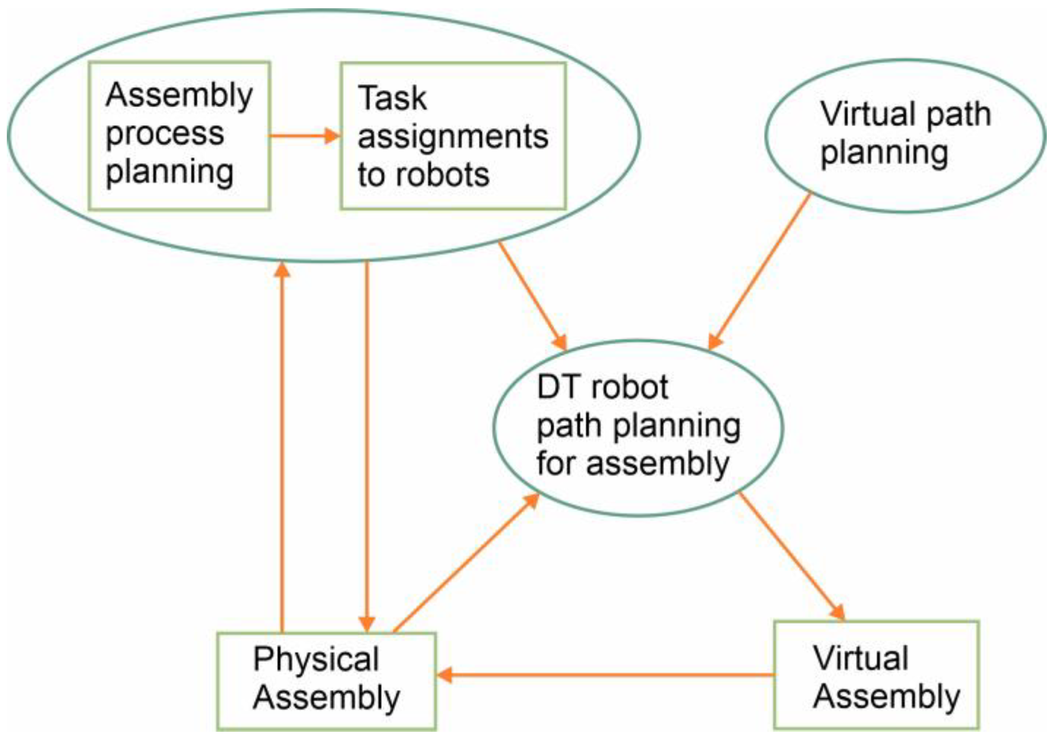
2.1. Digital Twin

In this section, the creation of the DT model for the path planning optimization of collaborative robots in the assembling process is analyzed. DT technology enables the development of smart assembly through the exchange of information between real and virtual environments. However, when multiple robots are involved in the assembly process and they need to operate in the same environment without collisions, a new challenge emerges with the attainment of interoperability between the virtual and physical data structure at the system level.

The design of industrial DTs can be established on the architectures of the industrial Internet of Things (IIOT) [45]. IIOT can operate as a connection between the physical world and DT [46]. Saemaldahr et al. [47] presented several architectures for IIOT, such as Industrial Internet Reference Architecture (IIRA) [48], IoT by Guth et al. [49], and WSO2 [50]. Among these architectures, Breivold emphasizes that only IIRA can contribute to the development of DT [51]. The IIRA standard was adapted, leveraging its capability to exchange data not only with the factory system but also with other DTs to meet the objectives of the presented DT. The proposed DT approach consists of five phases. Figure 1 summarizes the five phases of the presented DT and their interrelations.

2.1.1. Physical Assembly Task Assignment for Every Robot

The assignment of the physical processes that each robot will perform in the smart assembly process is essential for the creation of the DT model. The sequence and type of each task are determined by the physical assembly process. The allocation of the tasks determines the tools attached to the robot’s end effector and the critical point locations that the robot must navigate for the successful deployment of the tasks.

2.1.2. Virtual Path Planning Process

The information physically captured information by each robot is accurately transferred into a virtual environment. In the digital environment, it is feasible to simulate, evaluate, generate, and optimize paths without causing any damage to the assets of the physical world. This is particularly valuable in robotics because the process of finding the optimal path requires several trials, mistakes in which can be costly. The virtual environment serves as a safe testing environment without interrupting the flow of the production process, and the resulting data can be incorporated into other optimization and monitoring stages of the production procedure.

2.1.3. Digital Twin Platform System

The DT platform serves as the fundamental pillar of DT. It implements all the information, models, and algorithms about the assembly procedure. This collective approach ensures that the scheduling of assembly activities and the creation of robotic paths can be approached holistically, rather than as separate tasks. Within the platform, the capabilities of controlling processes, machines, and their positions through 3D models are implemented. In this way, the procedures of simulation, improvement, and analysis of industrial procedures can be successfully performed.

2.1.4. Digital Twin Process Data

The data gathered in the DT platform system is processed to produce new information. The DT platform accurately represents real-world conditions and physical models of the assembly process. This information is combined with digital data and algorithms for additional processing to determine paths that are consistent with real-world conditions. The DT model and simulation platform enable the adjustment of the robot’s trajectory and facilitate the responsiveness and the study of the whole system. The final path is converted into the appropriate programming language so that it can be executed by the robot.

2.1.5. Communication and Connectivity

A critical aspect of developing the DT model is the establishment of its communication with the real-world assets. The utilization of industrial protocols, such those described in [52], can contribute to monitor the assembly procedures in detail. The implementing industrial networks are classified into 3 main categories: Fieldbus networks, Ethernet-based networks and wireless industrial networks that use technologies such as Wi-Fi, Bluetooth or Zigbee [53].

The interconnection of assembly information, robot path planning and the physical world can be achieved by utilizing DT technology. Figure 2 shows the proposed DT framework for the path planning optimization of robotic arms in the assembly process. It consists of three layers: the physical, the virtual, and the interaction layer. The elements of each layer and their interactions are further analyzed.

The physical layer contains the entities and information encountered in the industrial environment. The physical entities may include machinery, robotic arms, assembly components, or other structural elements in the environment. It is necessary to track the location of these elements throughout time and observe any changes in their state. The information encountered in the physical world concerns the sequence of assembly processes, the speed of robot movement, and the availability of components. The overall system is formed by many physical entities and pieces of information that are correlated with each other. This data can be collected by appropriately placing cameras or sensors in the various areas of the production process. Their optimal positioning and the processing of their signals are outside the scope of the present paper.

The digital layer contains all the digital information related to the execution of tasks. This information is classified into assembly-related and path planning related information. The assembly-related information embraces the assembly specifications, the design of the components, and the assembly simulation confirmation. The path planning related information includes the position of O(0,0,0) of each robot’s coordinate system and the path it can execute to accomplish its mission. The origin O(0,0,0) is specified by the robot’s manufacturer. It is situated at a fixed predetermined position, on or close to the robot’s structural frame.

The interaction layer manages physical and digital information. Information management incorporates data collection, pre-processing, finding the optimal path, trajectory extraction, and data sharing. Following the completion of the assembly of a product, the data processing operation for the subsequent step takes place. The data pre-processing is performed to eliminate the noise, clean the data and structure the data [54]. Next, all the data from assembly path planning and environmental modeling are merged together in a data-driven relation for carrying out the path planning optimization procedure. Finally, the trajectory for each robot is extracted based on the resulting path and the data sharing through the communication network is accomplished.

Figure 3 describes the methodology for utilizing data from the DT and the process for the path planning process. Initially, data from the physical layer is input into the interaction layer to construct the robot’s virtual operating environment. In the interaction layer, the data from the virtual environment is interpreted and that associated with the static configuration of the physical environment is selectively transferred to the digital layer. In the digital layer, the movement paths of each robot are designed separately, without taking into account the movements of the other robots or possible changes in the environment. The 3D paths are generated using the AFSA, according to [55]. Then, the process of detecting a possible collision between the robots is carried, out taking advantage of the tools in NVIDIA Omniverse. This process is only employed for robots that operate in the same environment or when their operating space dynamically changes. AFSA and detection of possible collisions are further analyzed in Section 2.3. If there is a collision between the robots, then 4D path planning is performed, as described in [44]. Each robot executes its planned trajectory based on a coordinate system whose origin is defined by its manufacturer. After the path planning is completed, the coordinates of the path points are transferred to the robot’s local coordinate system, according to the correlation of the cartesian coordinate transformation procedure [56]. The final stage contains the creation of the robot’s trajectory.

The behavior of static physical models is determined through behavioral modeling. The physical behavior of each element can be described by differential equations and their motion in space over time can be precisely determined through kinematic and dynamic analysis [57,58]. The behavior of six-degree-of-freedom industrial robotic arms is simulated using the Denavit–Hartenberg (DH) notation. DH notation defines the kinematic equations of the robot by specifying the position and attitude of its end effector over a determined coordinate system [59]. The determination of the robot’s position for its input in the DT is accomplished by solving the forward kinematic problem through the numerical real-world values of the robot’s joint angles. The extraction of the trajectory is achieved from the coordinates of the points that resulted from the path planning process through the solution of the inverse kinematic problem [60].

The simulation of the real world in a DT requires the acquisition of vast and different data. High-resolution spatial and temporal data are essential for reproducing both static and dynamic real-world assets. As the volume and resolution of data increases, the computational demands required for processing, developing and maintaining a DT model increase correspondingly. Intensive data collection might make model administration and management difficult. Thus, it is essential to capture only the data that affects the functionality of the DT and industrial process.

The operation of industrial machinery, particularly robotic arms, is regulated by an advanced physics model. The machines consist of multiple components of different sizes that are related to each other through their structural and kinematic models. The components of each machine are actuated using electrical, mechanical, hydraulic, or other mechanisms. The relationship between the components and the actuated procedures can be replicated in detail virtually in the corresponding model of each machine. However, their detailed representation in the digital model significantly increases the required computations and the model’s size, without contributing equally to the examination of path planning and assembly procedures. Therefore, the detailed representation of these processes is excluded from the presented approach without compromising the accurate representation of the functionality, kinematic motion, and spatial configuration of the machines.

The representation of DT is vital to reflect the real-world conditions in a realistic and computational efficient way. In the real world, there are some constraints that define the operation of the mechanisms. The moving elements of mechanisms are dependent on the movement of other parts or their limited range of motion. These constraints are simulated to the DT by defining the motion of the connected components or limiting their motion range. The behavior of the mechanism and objects contained in the DT’s environment are also aligned with the established law of physics, such as gravity. The dimensions of physical objects are maintained through the parameters of the digital model’s size. The parameters define in the virtual environment the length, the size or the shapes of the physical objects. The distances between elements in the digital environment are precisely equivalent to those in the real world, which is achieved by appropriately locating them. The numerical values of the dimensions of the building structures and the interior layout are precisely determined by the physical environment. Information about doors, windows, and lights are not maintained, on the condition that they do not restrict or interfere with the movements of robots, people, or other machines in the environment.

The environmental representation of the DT must be associated with the path planning algorithm so that they can communicate seamlessly. The path planning algorithm uses a process to simplify the complex 3D geometric shapes encountered in industrial spaces and create a computationally optimal environment for searching for the optimal solution. The simplification is performed to an extent that does not affect finding the optimal path. Machine models are represented by complex geometries that must be reduced for representation in a grid environment. Consistency between the environments in the DT and the path planning algorithm is ensured through the delimitation of machines by key points. The key points are employed to define the boundaries and dynamic behavior of the machines in the grid environment. They are points specified by a set of coordinates that are utilized for describing the volumetric representation and the locations of the machine’s components. They are placed in fixed positions to accurately describe the boundaries and shape of the machine volumes. Key points preserve essential information regarding the machines’ location, geometry, and operational behavior. Two kinds of key points are used to distinguish static and dynamic parts. They also separate the fixed and moving volumes of the machines. Figure 4 shows an example of the key points’ placements in purple. The static and dynamic obstacles in the path planning algorithm’s grid environment are determined based on the location and type of key points. Kinematic models of machines are used to determine the spatial trajectory of moving elements as a function of time. Thus, the impact of their motion on the environment is determined. The robot’s path is determined based on the environmental information of the DT. This information, combined with the spatial configuration of all the assets in the DT environment, can be used as a collision detection mechanism. The resulting path from the path planning algorithm is simulated in the DT environment. Figure 5 shows the interaction between the path planning algorithm and the DT.

The presented DT was built in Nvidia Omniverse [61]. Nvidia Omniverse allows the visualization and precise representation of the physical world in a digital safe environment. Moreover, it provides the capability of managing the elements of the virtual environment and analyzing the information.

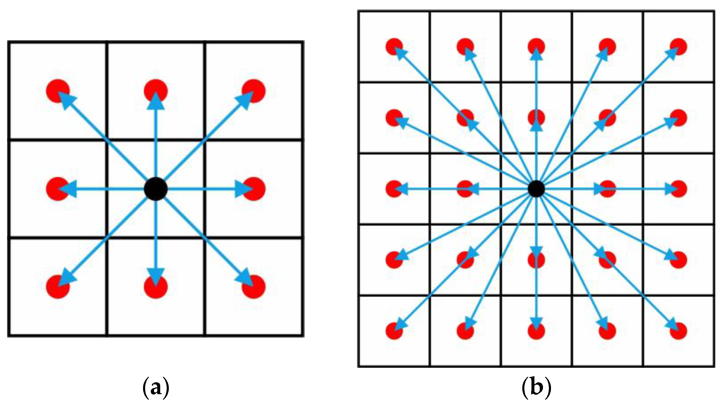
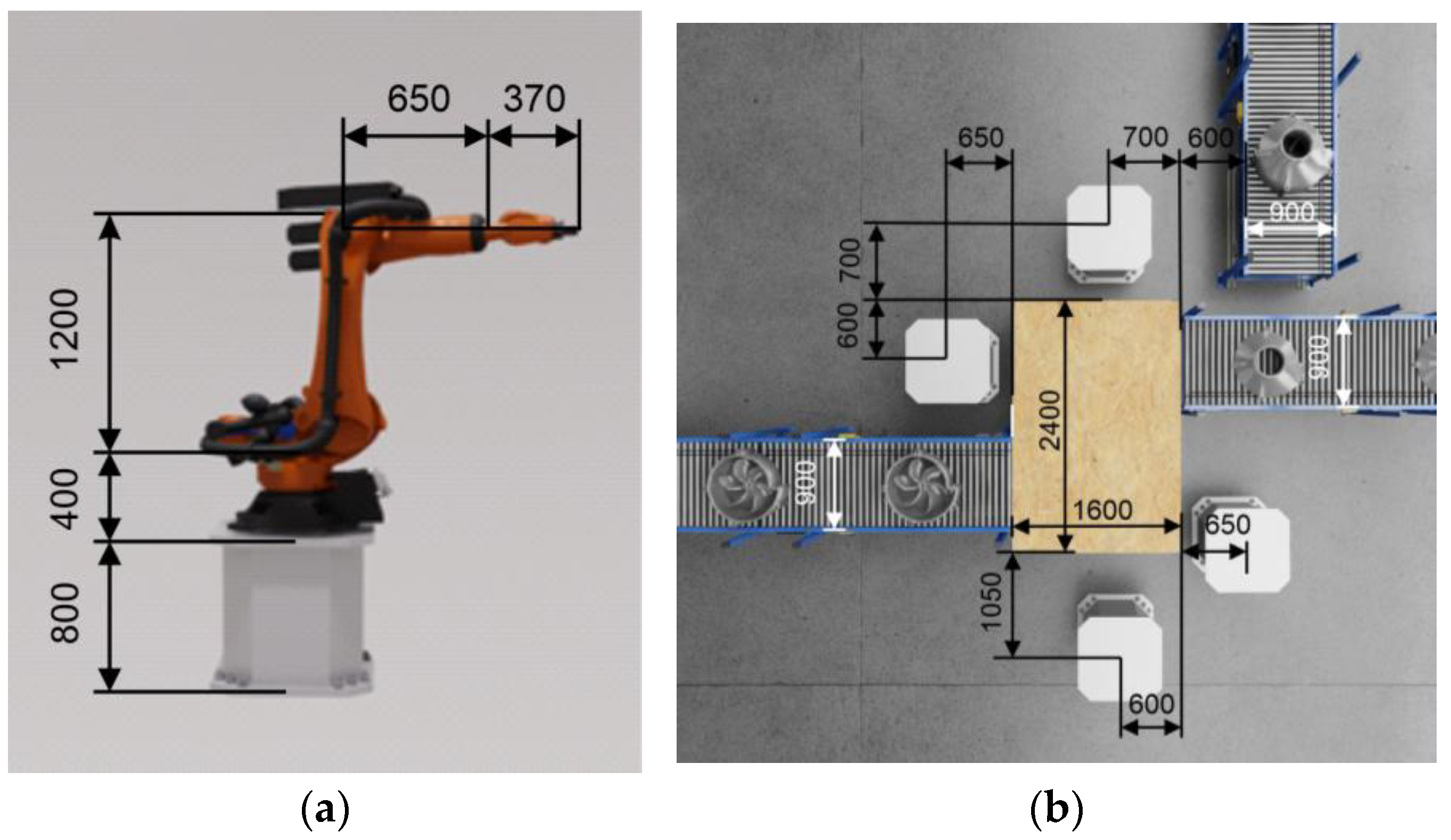
2.2. Modeling of the Environment

The 4D grid method is employed to simulate digitally the environment of the path planning algorithm. This approach incorporates the time variable into a 3D grid, allowing the monitoring of changes occurring in the modeled environment over time. The 3D grid enables the representation of the equipment met in the physical industrial environment. The 3D grid divides the physical space into many 3D elementary parallelepipeds. All 3D parallelepipeds have the same dimensions. Each elementary parallelepiped is represented by a discrete point located on its centroid. Temporal information is stored for each discrete point. Figure 6a and Figure 6b show an example of an elementary parallelepiped, with its discrete point and 3D environment, respectively.

The discrete point can be in the free or the obstacle state. The free state allows the robot to be transferred to the discrete point, while the obstacle state prohibits any movement on its representing volume. At a given time, the discrete point can be only in one state. These states enable the simulation of obstacles that are often encountered in industrial environments.

The size of the grid environment is determined based on the tasks that are planned to be performed. The dense mesh represents space more accurately and is ideal for tasks where precision to the robot’s movement or detailed tracking of an area’s changes is required. The denser the grid, the higher the computational requirements and the volume of information are. The thin grid is used in cases where the robot needs to move at a higher speed without emphasizing the accuracy of its position or its path. Some examples of these cases are encountered in pick and place tasks or when the robot needs to completely change its working position. The thin grid is ideal in circumstances where large objects are located in the environment or large areas need to be tracked. Nevertheless, the thin grid represents spaces less accurately and the robot’s generated trajectory does not accurately take into account the details of the environment.

Obstacles encountered in the environment where collaborative robots operate can be classified into two types: static and dynamic. Static obstacles retain their position and form unchanged over time. They represent unmovable elements in the environment, such as walls or permanent structures. Dynamic obstacles are time-dependent, with their existence varying over time. They can be used to simulate moving elements, such as moving items or the machinery’s components. Humans engaged in production processes and located in the robot’s workspace are modeled as dynamic obstacles to reflect their mobility.

In the grid environment, the discrete points defined as static obstacles remain in the obstacle state throughout the entire evolution of the algorithm, while the state of the discrete points defined as dynamic obstacles changes from free to obstacles and vice versa over time. The discrete points are defined as obstacles or free with the numbers 0 and 1 respectively. The influence of the temporal variable on the environment’s morphology is expressed through the dynamic obstacles.

The grid environment can either represent the entire industrial environment or only a smaller subsection of it where the robots perform the allocated tasks. Figure 7a demonstrates an example where the grid environment represents the entire working space. Figure 7b shows an example where the robot operating area is isolated from the entire workspace and represented by the 3D grid environment.

The end effectors of industrial robotic arms can move precisely in a 3D environment along all three principal axes, x, y and z. In the path design process, it is necessary to digitally simulate their multidirectional capabilities. Simulation in the grid environment is achieved through the utilization of the 24 possible movement navigation model. In a grid environment, researchers usually employ the 8 possible movement points navigation model. The 8 possible movement point model allows the robot to move in 8 different directions, while the 24 possible movement point model allows the movement in 16 different directions. The additional movement directions, as well as the ability to move to additional points that are located further from the given movement point provided by the 24 possible movement model, can be beneficial to the path formation and reduce the length of the formed path [62]. More details about the 24 possible movement point model, regarding to the length reduction, the computational requirements and its impact on path formation, can be found in [62]. Figure 8a and Figure 8b represent an example of 8 and 24 possible movement points navigations models, respectively. The agent, in addition to the points depicted in the model of 24 possible movement points, can also move to the points along the z-axis, as described in [55].

2.3. Artificial Fish Swarm Algorithm

AFSA is a nature inspired metaheurestic stochastic algorithm that is proposed in [63]. AFSA is characterized by its flexibility, robustness to faults, and insensitivity to initial conditions. In addition, it exhibits rapid convergence, a strong global search ability, high precision, and robust performance [64].

AFSA imitates four behaviors of a fish swarm observed in nature. AFSA utilizes these behaviors to find the optimal path. Preying, swarming, following, and random behavior are used for selecting the next possible movement point of artificial fish.

Preying behavior allows the fish to select the next possible movement point according to Equation (1). It checks whether the value of the objective function Y_j is greater than the value of the Y_i. X is the fish location and Y is the value of the objective function. The indexes i and j indicate the current and the next point of the fish, respectively. If the Y_j > Y_i, the artificial fish will move one step closer to the selected location according to Equation (2); otherwise, it will again choose the next possible movement point via Equation (1). The process of searching of the next possible movement points is repeated until a point with higher value of objective function is found or the reselection number is higher than an attempt number parameter, fishTryNum. If a better position is not found, the random behavior is executed. In Equation (2) ||X_j-X_i|| = d_ij is the distance between the current location i and the next possible j.

$${\mathrm{X}}_{\mathrm{j}}(\mathrm{t}+1) ={\mathrm{X}}_{\mathrm{i}}\left(\mathrm{t}\right)+\mathrm{Visual} \times \mathrm{Rand}\left(\right),$$

(1)

$${\mathrm{X}}_{\mathrm{i}} (\mathrm{t}+1)={\mathrm{X}}_{\mathrm{i}} \left(\mathrm{t}\right)+{\displaystyle \frac{{\mathrm{X}}_{\mathrm{j}}\left(\mathrm{t}\right)-{\mathrm{X}}_{\mathrm{i}}\left(\mathrm{t}\right)}{‖{\mathrm{X}}_{\mathrm{j}}\left(\mathrm{t}\right)-{\mathrm{X}}_{\mathrm{i}}\left(\mathrm{t}\right)‖}} \times \mathrm{Step} \times \mathrm{Rand}\left(\right),$$

(2)

In swarming behavior, the artificial fish explores the environment within its range by evaluating the number of fishes located in its current searching area. The fish uses Equation (3) to calculate the center position based on the distribution of the other fish. The center position is selected if its objective function value is higher than its current position and if it is not too crowded. In Equation (3), n_f indicates the number of fish in the examined area. The crowding degree of the fish in the examined position, δ ∈ (0,1) is calculated using Equation (4). If any of the above conditions are not met, preying behavior is executed. If the center point aligns with the aforementioned conditions, the fish moves one step towards the central position according to Equation (5).

$${\mathrm{X}}_{\mathrm{c}}={\sum }_{\mathrm{j}=1}^{{\mathrm{n}}_{\mathrm{f}}}{\displaystyle \frac{{\mathrm{X}}_{\mathrm{j}}}{{\mathrm{n}}_{\mathrm{f}}}},$$

(3)

$${\displaystyle \frac{{\mathrm{n}}_{\mathrm{f}}}{\mathrm{N}}}\le \mathsf{\delta },$$

(4)

$${\mathrm{X}}_{\mathrm{i}}(\mathrm{t}+1)={\mathrm{X}}_{\mathrm{i}}(\mathrm{t})+{\displaystyle \frac{{\mathrm{X}}_{\mathrm{C}}\left(\mathrm{t}\right)-{\mathrm{X}}_{\mathrm{i}}\left(\mathrm{t}\right)}{‖{\mathrm{X}}_{\mathrm{C}}\left(\mathrm{t}\right)-{\mathrm{X}}_{\mathrm{i}}\left(\mathrm{t}\right)‖}}\times \mathrm{S}\mathrm{t}\mathrm{e}\mathrm{p}\times \mathrm{R}\mathrm{a}\mathrm{n}\mathrm{d}(),$$

(5)

In following behavior, the artificial fish observes the position of the other fish within its vision field. If the value of the objective function in optimal position is higher than the current position and the position is not crowded, the artificial fish moves one step towards to the optimal position according to Equation (6). If the above conditions are not satisfied, the artificial fish performs prey behavior.

$${\mathrm{X}}_{\mathrm{i}}(\mathrm{t}+1) ={\mathrm{X}}_{\mathrm{i}}\left(\mathrm{t}\right)+{\displaystyle \frac{{\mathrm{X}}_{\mathrm{j}}\left(\mathrm{t}\right)-{\mathrm{X}}_{\mathrm{i}}\left(\mathrm{t}\right)}{‖{\mathrm{X}}_{\mathrm{j}}\left(\mathrm{t}\right)-{\mathrm{X}}_{\mathrm{i}}\left(\mathrm{t}\right)‖}} \times \mathrm{Step} \times \mathrm{Rand}\left(\right),$$

(6)

In random behavior, the fish moves randomly to a position in its visual field according to Equation (7). In this study, instead of random behavior, a behavior proposed in [62] was utilized.

$${\mathrm{X}}_{\mathrm{i}}(\mathrm{t}+1) ={\mathrm{X}}_{\mathrm{i}}\left(\mathrm{t}\right)+\mathrm{Step} \times \mathrm{Rand}\left(\right),$$

(7)

The objective function used for the evaluation of the next possible movement point is the same as [44] and presented in Equation (8). The coefficients w1, w2, w3 and w4 represent the importance of the terms of the distance of the discrete point’s location to the ending point, the safety’s value factor, the total movement point factor, and the safety’s value of dynamic obstacles, respectively. The safety value and total movement point factor are calculated according to Equations (9) and (10), respectively, where k represents the total number of the discrete points from the position where the fish is located, g the total number of obstacles from the same location, and w the number of discrete points eliminated due to interference of an obstacle between the fish’s location and the set of possible movement point. The safety value of dynamic obstacles is introduced as shown in Equation (11), where d is the total number of dynamic obstacles from the position of the fish.

$$\mathrm{f}\left(\mathrm{x}, \mathrm{y}, \mathrm{z}\right) ={\sqrt{{\left({\mathrm{x}}_{\mathrm{i}}-{\mathrm{x}}_{\mathrm{ending}}\right)}^2+{\left({\mathrm{y}}_{\mathrm{i}}-{\mathrm{y}}_{\mathrm{ending}}\right)}^2+{\left({\mathrm{z}}_{\mathrm{i}}-{\mathrm{z}}_{\mathrm{ending}}\right)}^2}}^{\mathrm{w}1}\times {\left({\displaystyle \frac{1}{\mathrm{S}\left({\mathrm{x}}_{\mathrm{i}},{\mathrm{y}}_{\mathrm{i}},{\mathrm{z}}_{\mathrm{i}}\right)}}\right)}^{\mathrm{w}2}\times {\left({\displaystyle \frac{1}{\mathrm{T}\left({\mathrm{x}}_{\mathrm{i}},{\mathrm{y}}_{\mathrm{i}},{\mathrm{z}}_{\mathrm{i}}\right)}}\right)}^{\mathrm{w}3}\times {\left({\displaystyle \frac{1}{\mathrm{D}\left({\mathrm{x}}_{\mathrm{i}},{\mathrm{y}}_{\mathrm{i}},{\mathrm{z}}_{\mathrm{i}}\right)}}\right)}^{\mathrm{w}4},$$

(8)

$$\mathrm{S}({\mathrm{x}}_{\mathrm{i}},{\mathrm{y}}_{\mathrm{i}},{\mathrm{z}}_{\mathrm{i}})={\displaystyle \frac{\mathrm{k}-\mathrm{g}}{\mathrm{k}}},$$

(9)

$$\mathrm{T}({\mathrm{x}}_{\mathrm{i}},{\mathrm{y}}_{\mathrm{i}},{\mathrm{z}}_{\mathrm{i}})={\displaystyle \frac{\mathrm{k}-\mathrm{w}}{\mathrm{k}}},$$

(10)

$$\mathrm{D}({\mathrm{x}}_{\mathrm{i}},{\mathrm{y}}_{\mathrm{i}},{\mathrm{z}}_{\mathrm{i}})={\displaystyle \frac{\mathrm{k}-\mathrm{d}}{\mathrm{k}}},$$

(11)

The methodologies of the navigation heatmap model, 3D simple and advanced elimination proposed in [55] were adopted. The integration of AFSA and the ray casting algorithm with time variable was achieved according to [44].

The calculation of the current time, t_cu is carried out through Equation (12). The variable V_cu is the arithmetical value of the robot’s speed and d_tr is the traveled distance between fish location and the next point and is calculated according to Equation (13). In Equation (13), x, y, z indicate the coordinates of the discrete point and indexes located and next imply the current and the next location of the fish. The coefficients q_DO and q_V are also utilized for cases where changes happen to dynamic obstacles and the robot’s speed, respectively. These coefficients assist in avoiding potential collision with dynamic obstacles and reduce the computational requirements. These coefficients are related to the time at which changes in the environment occur and are utilized through Equations (14) and (15). The variables t_DO and t_V are the time of changes occurring to dynamic obstacles and robot’s velocity, respectively. The detection of collisions between robots and dynamic obstacles integrating the ray casting algorithm with AFSA is performed by precisely calculating the collision time between the robot and the dynamic obstacle. This procedure includes the calculation of temporal time variable t_temp correlating the current time and required time that fish needs to travel from its current location to the collision coordinates. The procedure is analyzed in detail in [44].

$${\mathrm{t}}_{\mathrm{cu}}={\mathrm{t}}_0+{\displaystyle \frac{{\mathrm{d}}_{\mathrm{tr}}}{{\mathrm{V}}_{\mathrm{cu}}}},$$

(12)

$${\mathrm{d}}_{\mathrm{t}\mathrm{r}}=\sqrt{{\left({\mathrm{x}}_{\mathrm{located}}-{\mathrm{x}}_{\mathrm{next}}\right)}^2+{\left({\mathrm{y}}_{\mathrm{located}}-{\mathrm{y}}_{\mathrm{next}}\right)}^2+{\left({\mathrm{z}}_{\mathrm{located}}-{\mathrm{z}}_{\mathrm{next}}\right)}^2},$$

(13)

$${\mathrm{t}}_{\mathrm{c}\mathrm{u}}\ge {\mathrm{q}}_{\mathrm{D}\mathrm{O}}\times {\mathrm{t}}_{\mathrm{D}\mathrm{O}},$$

(14)

$${\mathrm{t}}_{\mathrm{c}\mathrm{u}}\ge {\mathrm{q}}_{\mathrm{V}}\times {\mathrm{t}}_{\mathrm{V}},$$

(15)

The total time required for a task to be performed by a robot was calculated according to Equation (16).

$${\mathrm{t}}_{\mathrm{t}}={\mathrm{t}}_{\mathrm{p}}+{\sum }_{\mathrm{i}}{\mathrm{n}}_{\mathrm{i}}\times {\mathrm{t}}_{\mathrm{i}},$$

(16)

In Equation (16), the variable t_t indicates the total time required for a robot to perform an operation cycle, t_p is the total time required for the path execution, the index i indicates the different assigned tasks that a robot performs, n_i is the number of times each task was repeated in the examined case, and t_i is the required time to perform the task. Tasks are performed only when the robot is positioned at a discrete point and not during its transit between different discrete points. The time t_p is calculated according to the t_cu calculation methodology presented in [44].

3. Results

The presented approach was applied for an assembly scenario where four industrial robotic arms are involved. The three robotic arms operate on assembling a product while the fourth performs manufacturing tasks in the same cell. The performed tests were conducted only in a simulation environment. Figure 9a,b show the dimensions (in millimeters) of the employed robots and the top view of the experimental setup, respectively. Figure 10 shows the assembly task of each robot and the corresponding performed sequence. The first and second robot are assigned with the task of picking two assembly components from separate conveyors and placing them at predefined positions. The component transported by the second robot is required to be placed on top of the component transported by the first robot. The third robot executes a bolting operation along the perimeter of the assembled components. The fourth robot’s job is to package the assembled product. The final product must be picked and transferred to a new predetermined location by the fourth robot. The assembly of the final component can be performed either through a sequential or a parallel approach. In the sequential approach, the robots initiate their trajectory only after the previous robot has completed its task, while in the parallel approach, the trajectories are executed contemporaneously. Trajectory generation for the sequential approach can be performed in a static environment; however, it extends the assembly’s overall completion time. In the parallel approach, the overall duration of the assembly process is reduced but the avoidance of collisions becomes a complex assignment. Collisions can be prevented by adjusting the initiation time of each task and synchronizing the speed of all robots. Nevertheless, these methods prove ineffective or suboptimal when the speed of one or more robots differs and it is necessary to generate the trajectory based on the 4D path planning approach.

The parameters values of AFSA presented in [44] are the as follows: The maximum iteration number was set 70, the maximum number of steps of a formed path was equal to 22, the population size of the fish swarm was set to 90, the fish swarm number of attempts was 14, the crowding factor δ = 0.3 w1 = 4, w2 = 1.5, w3 = 0.9, w4 = 1.6, q_DO = 0.05 and q_V = 0.02. The heatmap parameters and the navigation strategy were the same as used in [44]. The experiment was conducted in a computer in which the CPU model was an Intel(R) Core(TM) i7-9750H 2.60 GHz (Intel, Santa Clara, CA, USA), the GPU model was a NVIDIA RTX2060 and with 16 GB RAM capacity (Nvidia, Santa Clara, CA, USA).

Figure 11a shows the DT modeling of the examined industrial environment. The modeling was carried out according to the methodology presented in Section 2. Figure 11b shows the 3D paths of the four robots in the same grid environment to perform the assigned tasks. The path from robot 1 is marked in green, from robot 2 in blue, from robot 3 in magenta, and from robot 4 in red. The discrete point in orange is a point at which a conflict between robots 2 and 3 may arise. The paths of robots 1 and 2 do not intersect each other; however, they share common intersection points with the path of robot 3. Thus, it is necessary to generate the 4D path of the third robot in order to optimize the process and avoid collisions. As the processes performed by the fourth robot at the examined time do not affect the paths of the remaining robots, its trajectory and positions are not represented in the 4D path finding.

In the examined case, the 3D grid represents the area where the operations of the robots are performed. It consists of 700 district points, each representing a volume of $150 \times 150 \times 125$ mm, with the total dimensions of the space being $1500 \times 1500 \times 875$ mm. The grid environment does not extend to the entire operational environment, but it is oriented to a localized region in proximity to the component and the generation of the inspected path. The components positioned by the robots on the workbench are classified as dynamic obstacles due to their periodic placement and removal by the robots. The volumes of the robots during the process of positioning the components and returning to their initial position to repeat their tasks are also defined as dynamic obstacles. The movement speed of robots 1, 2, and 4 were set to 25 mm/s, while for robot 3, movement speed was set to 70 mm/s. The paths of robots 1 and 3 are entirely represented within the grid environment, while the paths of robots 2 and 4 are only partially demonstrated, beginning from the moment they enter the examined grid. The examined time corresponds to the phase after the placement of the assembled parts by robots 1 and 2.

Figure 11c–e show the path execution and the positions of the robotic arm in the environment. Figure 11f shows a diagram containing the start and end time of each dynamic obstacle. Figure 11g shows the resulting path. The path traverses all locations where actions will be executed and concludes at a final position that does not obstruct the performance of subsequent tasks. Purple dots represent the dynamic obstacles in the examined environment and light blue the dynamic obstacles that represent the placement of the components. The path length of robot 3 in the case represented in Figure 11b was 1695.8 mm, while in the case of Figure 11g, it was 1896.3 mm. Although the resulting path is slightly increased, it enables the avoidance of collision. The deployment time for the path planning procedure is 43 s. Only the time required for the path planning was measured, as the DT environment had been established in advance. Figure 11h illustrates the duration required for each robot to complete the assigned task. It is worth noting that, in addition to the path’s execution time, the duration of each task was also calculated to the total required time. It was assumed that the placement of components requires 4 additional seconds, whereas the bolting operation requires 2 s. The execution duration of each robotic operation is calculated from the initial inauguration of its task, extending beyond the path illustrated in the examined grid environment. Figure 11h demonstrates that the operating time of robots 1 and 3 in executing the examined assembly is relatively shorter in comparison to robots 2 and 4, while their idle time until the repetition of the cycle is longer. These indications imply that the robots can be deployed for executing supplementary tasks within their operational environment.

4. Discussion

DT is a technology with major impact on the challenges of Industry 5.0. DTs facilitate the management of complex and large data, usually met in industrial processes. The implementation of DTs in the collaborative robot field can enhance their capabilities and efficiency. However, the creation and utilization of a DT system is challenging. The detailed representation of all industrial processes and assets digitally can lead to high computational demands. Therefore, DT scalability and administration become difficult. The elimination of non-essential data can decrease the computational demands and facilitate the DT management. The data elimination must be conducted in alignment with the objectives of the DT, because the inappropriate simplification of information can significantly affect its serviceability.

The presented approach of implementing path planning into a DT for the trajectory optimization of collaborative robots is particularly effective. The path planning algorithms can generate optimal paths in environments with static and dynamic obstacles. In cases where 3D path planning is insufficient, the employment of a 4D path planning algorithm is used to solve the problem optimally. The integration of a time variable to a 3D path to spatial planning allows the generation of paths in conditions that commonly arise in real-world industrial environments, like changes in a robot’s speed or the appearance of dynamic obstacles. The 4D path planning algorithm allows the robotic arms to operate simultaneously in the same workspace without collisions. The simulation of the resultant trajectory in the DT environment facilitates the detection of collisions with the robotic arm’s surroundings. Virtual testing provides a safe environment for evaluating alternative scenarios without causing damage to physical equipment.

The presented DT is deployed for the design, simulation and optimization of the trajectory of industrial robotic arms. The monitoring and adaptation of physical assets are accomplished by the replication of the physical parameters and kinematic behavior of systems in a virtual environment. Two way communication between the physical and digital environments is feasible through the parameters of the geometric characteristics of industrial robots and the numerical values of their joint angles. Thus, the synchronization between the DT and the physical equipment can be established.

The development of the proposed DT system can be further expanded and broaden the existing research field. Future research is recommended to concentrate on the following areas:

• Enriching the library of digital models of machinery while preserving their interaction and connectivity;
• Investigating the security, stability, and consistency of industrial networks, due to the large volumes of data transmissions between the physical and digital environments;
• The utilization of a DT establishes a direct interdependence between the DT and the execution of industrial processes. The handling of potential failures of the DT as the related communication and data collection infrastructures needs to be investigated;
• Leveraging the contribution of the presented study related to the path planning alongside the integration of a temporal variable to the DT system for optimizing the industrial production scheduling.

References

1. Maddikunta, P.K.R.; Pham, Q.V.; B, P.; Deepa, N.; Dev, K.; Gadekallu, T.R.; Ruby, R.; Liyanage, M. Industry 5.0: A Survey on Enabling Technologies and Potential Applications. J. Ind. Inf. Integr. 2022, 26, 100257. [Google Scholar] [CrossRef]
2. van Erp, T.; Carvalho, N.G.P.; Gerolamo, M.C.; Gonçalves, R.; Rytter, N.G.M.; Gladysz, B. Industry 5.0: A New Strategy Framework for Sustainability Management and Beyond. J. Clean. Prod. 2024, 461, 142271. [Google Scholar] [CrossRef]
3. Huang, S.; Wang, B.; Li, X.; Zheng, P.; Mourtzis, D.; Wang, L. Industry 5.0 and Society 5.0—Comparison, Complementation and Co-Evolution. J. Manuf. Syst. 2022, 64, 424–428. [Google Scholar] [CrossRef]
4. Leng, J.; Sha, W.; Wang, B.; Zheng, P.; Zhuang, C.; Liu, Q.; Wuest, T.; Mourtzis, D.; Wang, L. Industry 5.0: Prospect and Retrospect. J. Manuf. Syst. 2022, 65, 279–295. [Google Scholar] [CrossRef]
5. Fosso-Wamba, S.; Guthrie, C. Artificial Intelligence and Industry 4.0 and 5.0: A Bibliometric Study and Research Agenda. Procedia Comput. Sci. 2024, 239, 718–725. [Google Scholar] [CrossRef]
6. Adel, A.; Alani, N.H.; Jan, T. Factories of the Future in Industry 5.0—Softwarization, Servitization, and Industrialization. Internet Things 2024, 28, 101431. [Google Scholar] [CrossRef]
7. Tóth, A.; Nagy, L.; Kennedy, R.; Bohuš, B.; Abonyi, J.; Ruppert, T. The Human-Centric Industry 5.0 Collaboration Architecture. MethodsX 2023, 11, 102260. [Google Scholar] [CrossRef]
8. Leirmo, T.L. Digital Twins for Industry 5.0: Unlocking the Human Potential. Procedia CIRP 2024, 130, 761–766. [Google Scholar] [CrossRef]
9. Valette, E.; Bril El-Haouzi, H.; Demesure, G. Industry 5.0 and Its Technologies: A Systematic Literature Review upon the Human Place into IoT- and CPS-Based Industrial Systems. Comput. Ind. Eng. 2023, 184, 109426. [Google Scholar] [CrossRef]
10. Sahan, A.S.M.; Kathiravan, S.; Lokesh, M.; Raffik, R. Role of Cobots over Industrial Robots in Industry 5.0: A Review. In Proceedings of the 2nd International Conference on Advancements in Electrical, Electronics, Communication, Computing and Automation, ICAECA, Coimbatore, India, 16–17 June 2023. [Google Scholar] [CrossRef]
11. Feng, Z.; Hu, G.; Sun, Y.; Soon, J. An Overview of Collaborative Robotic Manipulation in Multi-Robot Systems. Annu. Rev. Control 2020, 49, 113–127. [Google Scholar] [CrossRef]
12. Correia Simões, A.; Lucas Soares, A.; Barros, A.C. Factors Influencing the Intention of Managers to Adopt Collaborative Robots (Cobots) in Manufacturing Organizations. J. Eng. Technol. Manag. 2020, 57, 101574. [Google Scholar] [CrossRef]
13. Galin, R.; Meshcheryakov, R. Automation and Robotics in the Context of Industry 4.0: The Shift to Collaborative Robots. IOP Conf. Ser. Mater. Sci. Eng. 2019, 537, 032073. [Google Scholar] [CrossRef]
14. Patil, S.; Vasu, V.; Srinadh, K.V.S. Advances and Perspectives in Collaborative Robotics: A Review of Key Technologies and Emerging Trends. Discov. Mech. Eng. 2023, 2, 13. [Google Scholar] [CrossRef]
15. Wang, X.V.; Kemény, Z.; Váncza, J.; Wang, L. Human–Robot Collaborative Assembly in Cyber-Physical Production: Classification Framework and Implementation. CIRP Ann. 2017, 66, 5–8. [Google Scholar] [CrossRef]
16. Wang, L.; Liu, S.; Liu, H.; Wang, X.V. Overview of Human-Robot Collaboration in Manufacturing. In Lecture Notes in Mechanical Engineering; Springer: Cham, Switzerland, 2020; pp. 15–58. [Google Scholar] [CrossRef]
17. Malik, A.A.; Bilberg, A. Collaborative Robots in Assembly: A Practical Approach for Tasks Distribution. Procedia CIRP 2019, 81, 665–670. [Google Scholar] [CrossRef]
18. Faccio, M.; Granata, I.; Minto, R. Task Allocation Model for Human-Robot Collaboration with Variable Cobot Speed. J. Intell. Manuf. 2024, 35, 793–806. [Google Scholar] [CrossRef]
19. Weingartshofer, T.; Bischof, B.; Meiringer, M.; Hartl-Nesic, C.; Kugi, A. Optimization-Based Path Planning Framework for Industrial Manufacturing Processes with Complex Continuous Paths. Robot. Comput. Integr. Manuf. 2023, 82, 102516. [Google Scholar] [CrossRef]
20. Larsson, S.; Kjellander, J.A.P. Path Planning for Laser Scanning with an Industrial Robot. Rob. Auton. Syst. 2008, 56, 615–624. [Google Scholar] [CrossRef]
21. Zhou, X.; Wang, X.; Xie, Z.; Gao, J.; Li, F.; Gu, X. A Collision-Free Path Planning Approach Based on Rule Guided Lazy-PRM with Repulsion Field for Gantry Welding Robots. Rob. Auton. Syst. 2024, 174, 104633. [Google Scholar] [CrossRef]
22. Abdelrahman, M.; Macatulad, E.; Lei, B.; Quintana, M.; Miller, C.; Biljecki, F. What is a Digital Twin anyway? Deriving the definition for the built environment from over 15,000 scientific publications. Build. Environ. 2025, 274, 112748. [Google Scholar] [CrossRef]
23. Malik, A.A.; Brem, A. Digital Twins for Collaborative Robots: A Case Study in Human-Robot Interaction. Robot. Comput. Integr. Manuf. 2021, 68, 102092. [Google Scholar] [CrossRef]
24. Ali, Z.; Biglari, R.; Denil, J.; Mertens, J.; Poursoltan, M.; Traoré, M.K. From Modeling and Simulation to Digital Twin: Evolution or Revolution? Simulation 2024, 100, 751–769. [Google Scholar] [CrossRef]
25. Daraba, D.; Pop, F.; Daraba, C. Digital Twin Used in Real-Time Monitoring of Operations Performed on CNC Technological Equipment. Appl. Sci. 2024, 14, 10088. [Google Scholar] [CrossRef]
26. Kreuzer, T.; Papapetrou, P.; Zdravkovic, J. Artificial Intelligence in Digital Twins—A Systematic Literature Review. Data Knowl. Eng. 2024, 151, 102304. [Google Scholar] [CrossRef]
27. Sifat, M.M.H.; Choudhury, S.M.; Das, S.K.; Ahamed, M.H.; Muyeen, S.M.; Hasan, M.M.; Ali, M.F.; Tasneem, Z.; Islam, M.M.; Islam, M.R.; et al. Towards Electric Digital Twin Grid: Technology and Framework Review. Energy AI 2023, 11, 100213. [Google Scholar] [CrossRef]
28. Wang, L. Digital Twins in Agriculture: A Review of Recent Progress and Open Issues. Electronics 2024, 13, 2209. [Google Scholar] [CrossRef]
29. Chomiak-Orsa, I.; Hauke, K.; Perechuda, K.; Pondel, M. The Use of Digital Twin in the Sustainable Development of the City on the Example of Managing Parking Resources. Procedia Comput. Sci. 2023, 225, 2183–2193. [Google Scholar] [CrossRef]
30. Ebni, M.; Bamakan, S.M.H.; Qu, Q. Digital Twin Based Smart Manufacturing; From Design to Simulation and Optimization Schema. Procedia Comput. Sci. 2023, 221, 1216–1225. [Google Scholar] [CrossRef]
31. Benfer, M.; Peukert, S.; Lanza, G. A Framework for Digital Twins for Production Network Management. Procedia CIRP 2021, 104, 1269–1274. [Google Scholar] [CrossRef]
32. Traini, E.; Antal, G.; Bruno, G.; De Maddis, M.; Lombardi, F.; Panza, L.; Spena, P.R. Hybrid Knowledge Based System Supporting Digital Twins in the Industry 5.0. Procedia Comput. Sci. 2024, 232, 1471–1480. [Google Scholar] [CrossRef]
33. Grieves, M.; Vickers, J. Digital Twin: Mitigating Unpredictable, Undesirable Emergent Behavior in Complex Systems. In Transdisciplinary Perspectives on Complex Systems: New Findings and Approaches; Springer: Cham, Switzerland, 2017; pp. 85–113. [Google Scholar] [CrossRef]
34. Kim, G.Y.; Kim, D.; Do Noh, S.; Han, H.K.; Kim, N.G.; Kang, Y.S.; Choi, S.H.; Go, D.H.; Song, J.; Lee, D.Y.; et al. Human Digital Twin System for Operator Safety and Work Management. IFIP Adv. Inf. Commun. Technol. 2022, 664, 529–536. [Google Scholar] [CrossRef]
35. Junnan, Z.; Jiangxin, Y.; Chongxin, Z.; Shuhan, L.; Anwer, N.; Yanlong, C. A Modeling Method of Complex Assembly Based on Digital Twin. Procedia CIRP 2022, 114, 79–87. [Google Scholar] [CrossRef]
36. Ma, Y.; Zhou, H.; He, H.; Jiao, G.; Wei, S. A Digital Twin-Based Approach for Quality Control and Optimization of Complex Product Assembly. In Proceedings of the 2019 International Conference on Artificial Intelligence and Advanced Manufacturing, AIAM 2019, Dublin, Ireland, 17–19 October 2019; pp. 762–767. [Google Scholar] [CrossRef]
37. Wang, J.; Yan, Y.; Hu, Y.; Yang, X.; Zhang, L. A Transfer Reinforcement Learning and Digital-Twin Based Task Allocation Method for Human-Robot Collaboration Assembly. Eng. Appl. Artif. Intell. 2025, 144, 110064. [Google Scholar] [CrossRef]
38. Zhang, D.; Leng, J.; Xie, M.; Yan, H.; Liu, Q. Digital Twin Enabled Optimal Reconfiguration of the Semi-Automatic Electronic Assembly Line with Frequent Changeovers. Robot. Comput. Integr. Manuf. 2022, 77, 102343. [Google Scholar] [CrossRef]
39. Zhang, Q.; Zheng, S.; Yu, C.; Wang, Q.; Ke, Y. Digital Thread-Based Modeling of Digital Twin Framework for the Aircraft Assembly System. J. Manuf. Syst. 2022, 65, 406–420. [Google Scholar] [CrossRef]
40. Du, Y.; Luo, Y.; Peng, Y.; Chen, Y. Industrial Robot Digital Twin System Motion Simulation and Collision Detection. In Proceedings of the 2021 IEEE 1st International Conference on Digital Twins and Parallel Intelligence, DTPI 2021, Beijing, China, 15 July–15 August 2021; pp. 196–199. [Google Scholar] [CrossRef]
41. Zhang, X.; Zheng, L.; Fan, W.; Ji, W.; Mao, L.; Wang, L. Knowledge Graph and Function Block Based Digital Twin Modeling for Robotic Machining of Large-Scale Components. Robot. Comput. Integr. Manuf. 2024, 85, 102609. [Google Scholar] [CrossRef]
42. Xuan, D.T.; Nam, L.G.; Viet, D.T.; Thang, V.T. A-Star Algorithm for Robot Path Planning Based on Digital Twin. In Lecture Notes in Mechanical Engineering; Springer: Singapore, 2022; pp. 83–90. [Google Scholar] [CrossRef]
43. Chen, Z.; Yuan, X.; Gu, Q.; Hu, C.; He, D. A Digital Twin System for 6DoF Robot Grasping. In Proceedings of the 35th Chinese Control and Decision Conference, CCDC 2023, Yichang, China, 20–22 May 2023; pp. 3292–3296. [Google Scholar] [CrossRef]
44. Chouridis, I.; Mansour, G.; Papageorgiou, V.; Mansour, M.T.; Tsagaris, A. Four-Dimensional Path Planning Methodology for Collaborative Robots Application in Industry 5.0. Robotics 2025, 14, 48. [Google Scholar] [CrossRef]
45. Awouda, A.; Traini, E.; Bruno, G.; Chiabert, P. IoT-Based Framework for Digital Twins in the Industry 5.0 Era. Sensors 2024, 24, 594. [Google Scholar] [CrossRef]
46. Attaran, S.; Attaran, M.; Celik, B.G. Digital Twins and Industrial Internet of Things: Uncovering Operational Intelligence in Industry 4.0. Decis. Anal. J. 2024, 10, 100398. [Google Scholar] [CrossRef]
47. Saemaldahr, R.; Thapa, B.; Maikoo, K.; Fernandez, E.B. Reference Architectures for the IoT: A Survey. Lect. Notes Data Eng. Commun. Technol. 2021, 72, 635–646. [Google Scholar] [CrossRef]
48. The Industrial Internet Reference Architecture—Industry IoT Consortium. Available online: https://www.iiconsortium.org/iira/ (accessed on 13 May 2025).
49. Guth, J.; Breitenbucher, U.; Falkenthal, M.; Leymann, F.; Reinfurt, L. Comparison of IoT Platform Architectures: A Field Study Based on a Reference Architecture. In Proceedings of the 2016 Cloudification of the Internet of Things, CIoT, Paris, France, 23–25 November 2016. [Google Scholar] [CrossRef]
50. A Reference Architecture for the Internet of Things. Available online: https://wso2.com/whitepapers/a-reference-architecture-for-the-internet-of-things/ (accessed on 13 May 2025).
51. Breivold, H.P. A Survey and Analysis of Reference Architectures for the Internet-of-Things. In Proceedings of the Twelfth International Conference on Software Engineering Advances, Athens, Greece, 8–12 October 2017. [Google Scholar]
52. Mashaly, M. Connecting the Twins: A Review on Digital Twin Technology & Its Networking Requirements. Procedia Comput. Sci. 2021, 184, 299–305. [Google Scholar] [CrossRef]
53. Lu, Y.; Liu, C.; Wang, K.I.K.; Huang, H.; Xu, X. Digital Twin-Driven Smart Manufacturing: Connotation, Reference Model, Applications and Research Issues. Robot. Comput. Integr. Manuf. 2020, 61, 101837. [Google Scholar] [CrossRef]
54. Tao, F.; Qi, Q.; Liu, A.; Kusiak, A. Data-Driven Smart Manufacturing. J. Manuf. Syst. 2018, 48, 157–169. [Google Scholar] [CrossRef]
55. Chouridis, I.; Mansour, G.; Papageorgiou, V.; Mansour, M.T.; Tsagaris, A. Enhanced Hybrid Artificial Fish Swarm Algorithm for Three-Dimensional Path Planning Applied to Robotic Systems. Robotics 2025, 14, 32. [Google Scholar] [CrossRef]
56. Lan, D.; Hanwei, Z.; Qingyong, Z.; Ruopu, W. Correlation of Coordinate Transformation Parameters. Geod. Geodyn. 2012, 3, 34–38. [Google Scholar] [CrossRef]
57. Hu, Y.; Zhao, X.; Wang, S.; Chiel, H.J.; Thomas, P.J.; Tarkhov, D.A.; Malykhina, G.F. Neural Network Modelling Methods for Creating Digital Twins of Real Objects. J. Phys. Conf. Ser. 2019, 1236, 012056. [Google Scholar] [CrossRef]
58. Liu, C.; Jiang, P.; Jiang, W. Web-Based Digital Twin Modeling and Remote Control of Cyber-Physical Production Systems. Robot. Comput. Integr. Manuf. 2020, 64, 101956. [Google Scholar] [CrossRef]
59. Yan, K.; Xu, W.; Yao, B.; Zhou, Z.; Pham, D.T. Digital Twin-Based Energy Modeling of Industrial Robots. Commun. Comput. Inf. Sci. 2018, 946, 333–348. [Google Scholar] [CrossRef]
60. Nicolescu, A.; Ilie, F.-M.; Tudor-George, A. Forward and inverse kinematics study of industrial robots taking into account constructive and functional parameter’s modeling. Proc. Manuf. Syst. 2015, 10, 157. [Google Scholar]
61. Omniverse Platform for OpenUSD | NVIDIA. Available online: https://www.nvidia.com/en-eu/omniverse/ (accessed on 25 May 2025).
62. Chouridis, I.; Mansour, G.; Tsagaris, A. Three-Dimensional Path Planning Optimization for Length Reduction of Optimal Path Applied to Robotic Systems. Robotics 2024, 13, 178. [Google Scholar] [CrossRef]
63. Lei, L.X.; Shao, Z.J.; Qian, J.X. An Optimizing Method Based on Autonomous Animats: Fish-Swarm Algorithm. Syst. Eng.-Theory Pract. 2002, 22, 32–38. [Google Scholar]
64. Zainal, N.; Zain, A.M.; Sharif, S. Overview of Artificial Fish Swarm Algorithm and Its Applications in Industrial Problems. Appl. Mech. Mater. 2015, 815, 253–257. [Google Scholar] [CrossRef]
Figure 1. DT’s phases and their interaction.
Robotics 14 00097 g001
Figure 2. Digital twin framework.
Robotics 14 00097 g002
Figure 3. Path planning procedure.
Robotics 14 00097 g003
Figure 4. Key point placement on models.
Robotics 14 00097 g004
Figure 5. Interaction between the path planning algorithm and the digital twin.
Robotics 14 00097 g005
Figure 6. Path planning grid environment: (a) 3D elementary parallelepiped with its discrete point; (b) 3D grid environment consisting of many 3D elementary parallelepipeds.
Robotics 14 00097 g006
Figure 7. Virtual environment represented in grid: (a) Grid environment represents the entire space; (b) Grid environment represents a smaller operation area.
Robotics 14 00097 g007
Figure 8. Possible point navigation models: (a) 8 possible navigation movement point model; (b) 24 possible navigation movement point model.
Robotics 14 00097 g008
Figure 9. Dimensions of robots and experimental setup: (a) Basic dimensions for the industrial robotic arm; (b) Dimensions of the experimental setup.
Robotics 14 00097 g009
Figure 10. Assembly task sequence.
Robotics 14 00097 g010
Figure 11. Resulting analysis of path deployment in the digital twin: (a) General configuration of assembly cell and robotic arms layout; (b) Initial path planning of robotic arms; (ce) Industrial robotic arms performing the resultant trajectory; (f) Diagram for delineating the starting and ending times of dynamic obstacles; (g) Path optimization results to avoid collisions; (h) Diagram of the operational durations of the robotic arms.
Robotics 14 00097 g011aRobotics 14 00097 g011b
Disclaimer/Publisher’s Note: The statements, opinions and data contained in all publications are solely those of the individual author(s) and contributor(s) and not of MDPI and/or the editor(s). MDPI and/or the editor(s) disclaim responsibility for any injury to people or property resulting from any ideas, methods, instructions or products referred to in the content.