Abstract
This study addresses the clinical requirements of a transoral surgery-assisting continuum robot. This application requires both high bendability and stiffness in order to ensure precise positioning and stable fixation of surgical tools. To meet these needs, we developed a tendon-driven discrete continuum robot unit featuring a ball–socket joint and superelastic Nitinol rods. One to three serially connected robot units were tested by applying proximal tendon tension () in the range of 100–1000 g while distal tension () was continuously increased to induce bending. During bending, the curves were interpolated using third-order to fifth-order polynomials at discrete levels. The interpolated inverse statics were validated experimentally and compared with finite element simulations using ANSYS. Furthermore, we propose a planar path planning algorithm and numerically evaluate it for a three-unit robot following an arc-shaped trajectory. The inverse statics successfully captured the nonlinear bending behavior of the tendon-driven robot. Validation experiments showed average angular errors of 2.7%, 6.6%, and 5.3% for one, two, and three connected units, respectively. The proposed path planning method achieved an average positional deviation from the reference trajectory ranging from 0.95 mm to 19.77 mm. This work presents a practical and generalizable experimental mapping framework for the inverse statics of tendon-driven discrete continuum robots, avoiding the need for complex analytical models.
1. Introduction
A continuum robot is defined as a snake-like robot which has continuous tangential vectors along its body [1]. Because of its slender shape and high bending capability, it can be used in aerospace [2,3], nuclear [4], and medical applications [5,6,7,8]. However, the slenderness and high bendability/dexterity of continuum robots can make actuation and control challenging compared with conventional rigid-body robots. Therefore, many actuation methods/mechanisms have been devised, including tendon-driven [9] and concentric tube [10] types, among others. For a recent survey of continuum robots, readers may refer to [11].
For medical applications, continuum robots can be introduced using a natural orifice such as the nose (transnasal), mouth (transoral), urethra (transurethral), or anus (transrectal). Such robots can be used to assist clinicians, providing enhanced dexterity and accuracy through a procedure called NOTES (Natural Orifice Transluminal Endoscopic Surgery) [12]. One important factor in continuum robots for assisting with transnasal surgery is a high bending angle with a low radius of curvature, which may not be met by commercialized transnasal surgery devices. For transoral surgery-assisting robots, clinical requirements include sufficiently high bendability and stiffness to allow for positioning and fixation of the surgery device with suitable orientation for the clinicians to perform surgery, along with high visibility and easy manipulability. Previous works [13,14] have designed high-stiffness continuum robots; however, these designs are limited to continuous robot units without adjustable stiffness.
To cope with these clinical requirements for transoral surgery-assisting continuum robots, we have developed a tendon-driven discrete continuum robot unit with a ball–socket joint [15]. A discrete continuum robot has a finite number of units connected with various joints, meaning that it has piecewise-continuous tangential vectors along its body. Because of high friction on the ball–socket joint’s contact surface, the developed discrete continuum robot has high stiffness and meets the clinical requirements of high stiffness and bendability. Moreover, two superelastic Nitinol rods with small diameters are inserted through the discrete continuum robot to make it bend uniformly. To control the configuration of the discrete continuum robot, the two tendons are pulled and released using a tangle/untangle-based strategy [16]. After adjusting the configuration, the stiffness of the discrete continuum robot is controlled by pulling a predefined finite amount of tendon displacement. However, this cycle of releasing tendons, adjusting the configuration, and pulling tendons makes control of the robot time-consuming and cumbersome. An alternatives is to control the discrete continuum robot with statics-based tendon tension control. However, exact analysis of the statics and inverse statics for the developed unit with superelastic Nitinol rods is not an easy task, and a preliminary study is required for full-fledged analysis. There are many statics-related works for continuum robots [11]. However, to the best of our knowledge, there are no previous works related to inverse statics for a discrete continuum robot unit with a ball–socket joint and superelastic Nitinol rods.
Therefore, in this work we propose the use of planar interpolated inverse statics for the tendon-driven discrete continuum robot unit with superelastic Nitinol rods. The proposed approach is conducted through experiments and represents an extended study of the previous work in [17]. In addition, dynamic analysis using Ansys 2024 R1 is performed to validate the experimental results and the inverse statics-based planar path planning for three serially connected units. This study provides a practical inverse statics estimation framework for tendon-driven discrete continuum robot units using piecewise planar approximation and experimental mapping, which avoids the need for complex analysis. Compared to analysis-based inverse statics methods, the proposed approach allows for real-time interpolation-based estimation with negligible computation cost, making it suitable for embedded implementation. In addition, the proposed methodology is readily adaptable to the inverse statics of similar tendon-driven discrete continuum robot units with various joint structures and stiffnesses.
The rest of this paper is organized as follows: the developed unit is explained in Section 2.1; the bending procedure of the unit under and tendon tension is explained in Section 2.2; Section 2.3 shows the experimentally-induced inverse statics; experimental validation of the proposed inverse statics, finite element method (FEM) results using Ansys, and planar path planning for three serially connected units are explained in Section 3; finally, the conclusions and outlook for future research are provided in Section 4.
2. Materials and Methods
2.1. Developed Unit
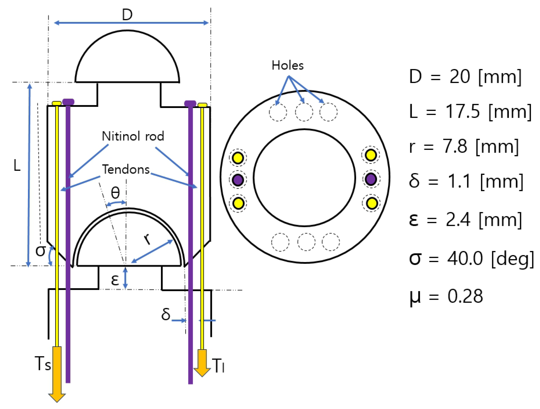
The schematics of the developed unit are presented in Figure 1. The left and right pictures in Figure 1 present side and top views of the unit, respectively. In the left picture in Figure 1, two units are connected through a ball–socket joint, with two tendons and two Nitinol rods passing through the two units.

Figure 1.
The schematics and main design parameters of the developed unit.
The major design parameters are also shown in Figure 1. Excluding the joint head, the unit has a diameter (D) of 20 mm, height (L) of 17.5 mm, and neck length () of 2.4 mm, with a maximum bending angle of 19.10 degrees. The ball and socket joint of the unit has a radius (r) of 7.8 mm. These dimensions were determined by clinical phantom dimension analysis. The static friction coefficient of the unit is 0.28, which is the same as an anodized aluminium surface. As can be seen in the top view picture in Figure 1, it has twelve holes of diameter 1.2 mm, which are located at 0°, 90°, 180°, and 270° angular positions, with three holes in each orientation. The yellow lines in Figure 1 represent tendons, which are fixed at the upper body of the unit, while the two purple lines represent Nitinol rods with diameter 0.89 mm. Each tendon passes through two passages; at the other sides of the tendon, the two tendon tensions and can be applied. The clearance between the Nitinol rod and the hole is 0.31 mm, which is an important design parameter for the bending stiffness and control of the unit.
2.2. Unit Bending Procedure Under and
In the initial setup of the two units in Figure 1, if equals , then the upper unit in Figure 1 is in a static equilibrium without bending. If is gradually increases, then the static equilibrium breaks at some value and the upper unit starts bending, which can be explained by Equation (1) below.
In Equation (1), and are respectively the maximum static frictional moment and static frictional moment between the ball and socket joint under and force application. Per Coulumb’s friction law, if < , then the upper unit is in static equilibrium status. If is gradually increased, then is increased accordingly; eventually, equals , which is in quasi-static status. If > by additional increase of , then the upper unit starts to rotate with dynamic frictional moment between the ball and socket interface. The exact calculation of and requires geometrical analysis and integration, which are currently in progress by the authors.
If the third condition in Equation (1) is satisfied, then the upper unit rotates. After rotation, the upper unit rotates without bending the Nitinol rod because of the 0.31 mm clearance between the Nitinol rod and the hole. If the movement amount of the upper unit exceeds the clearance, then the Nitinol rod starts to be deflected. The Nitinol rod continues to be deflected until static equilibrium is reached in the Nitinol rod and the upper unit. In the static equilibrium of the upper unit after rotation, the bending moment of the Nitinol rod exerted on the upper unit plus the static frictional moment equal the external moment exerted by and , which is presented in Equation (2).
In Equation (2), is the momentum resulting from and , while and are the moment resulting from deflection of the Nitinol rod and the static frictional moment between the ball and socket joint under and force application and the applied force from deflection of the Nitinol rod.
2.3. Experimentally Constructed Inverse Statics of One, Two, and Three Serially Connected Units
2.3.1. Inverse Statics of One, Two, and Three Serially Connected Units in the Bending Direction
The experimental setup is illustrated in Figure 2. The units are made of anodized aluminium with the physical dimensions and properties in Figure 1, as presented in the lower right side small picture in Figure 2. The lower unit is embedded in a 3D-printed black test apparatus and fixed with a bolt, as depicted in Figure 2. The upper units are placed on the lower unit with two Nitinol rods passing through the units, as described in Figure 1. As presented in Figure 2, the left-side tendon is connected to the weights and the right-side tendon is connected to the F/T sensor, which is mounted on the linear guide. The weights are placed at the end of the left-side tendon to apply tensions () to the tendon, as depicted in Figure 2. Here, is set to 100, 200, 300, 500, 700, 900, and 1000 g, while is slowly increased from the value by adjusting the linear guide position until the maximum bending angle is reached at all upper units. The maximum value of 1000 g was selected because this amount of tension force is considered sufficient to sustain clinical tools in real clinical situations while maintaining light weight and high manipulability. Measurement of is carried out using the F/T sensor shown in Figure 2.
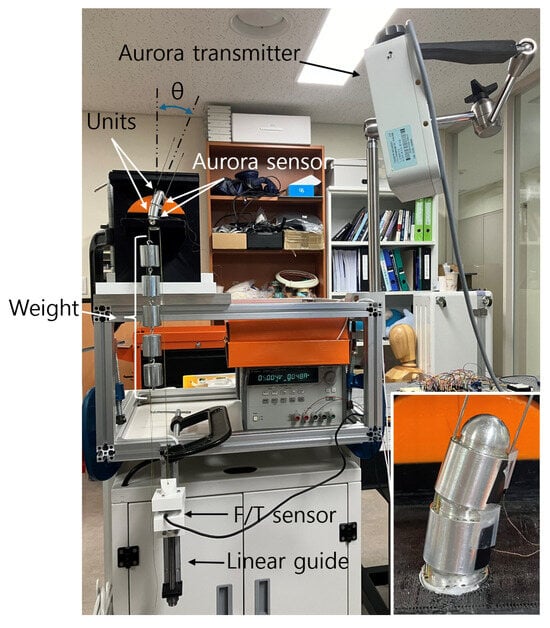
Figure 2.
Experimental setup.
The sensors of the electromagnetic tracking system (Aurora v2, NDI) are attached to the body of the upper units to measure the bending angle with the Aurora transmitter placed in front of the sensors, as presented in Figure 2. Data acquisition is performed by establishing serial communication between the Aurora sensor and a desktop PC. The data acquisition programming was carried out with QT Creator 4.2, MinGW-w64 setting in a Windows environment. To minimize the measurement error, the quaternion angle in the principal plane was calculated and calibrated at 0–19.0° before starting the experiment.
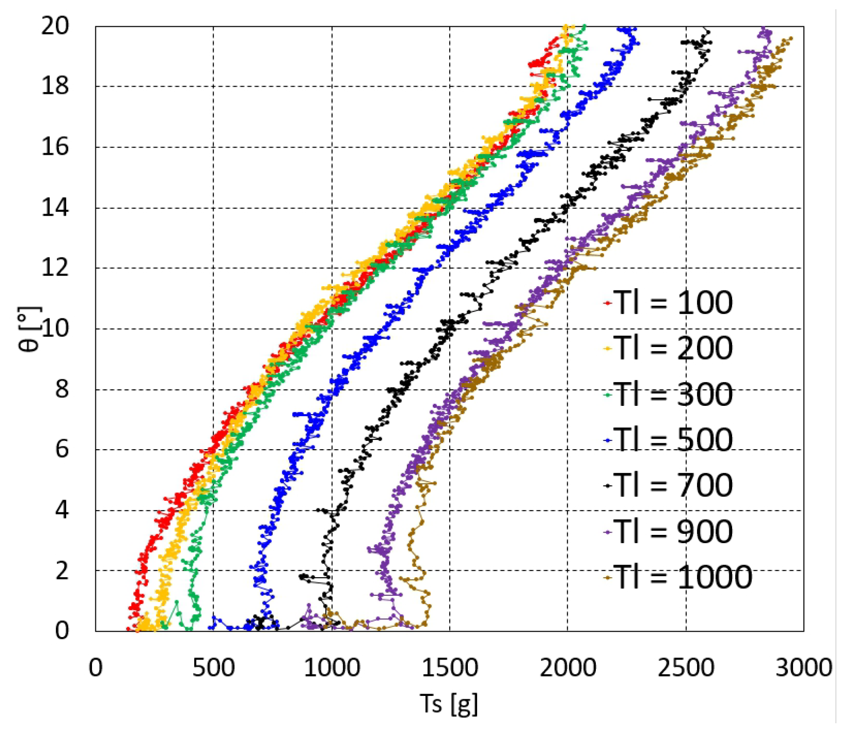
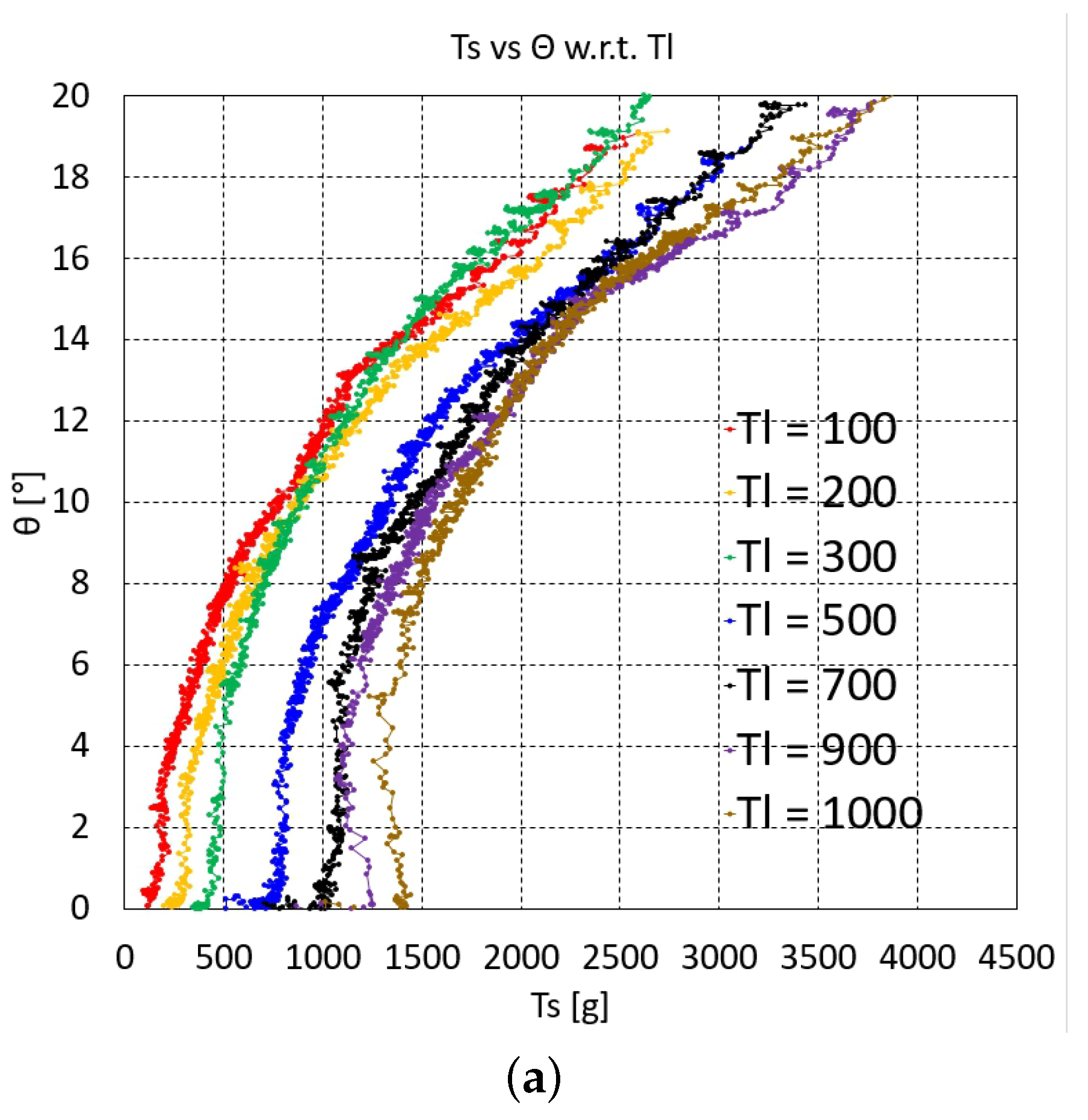
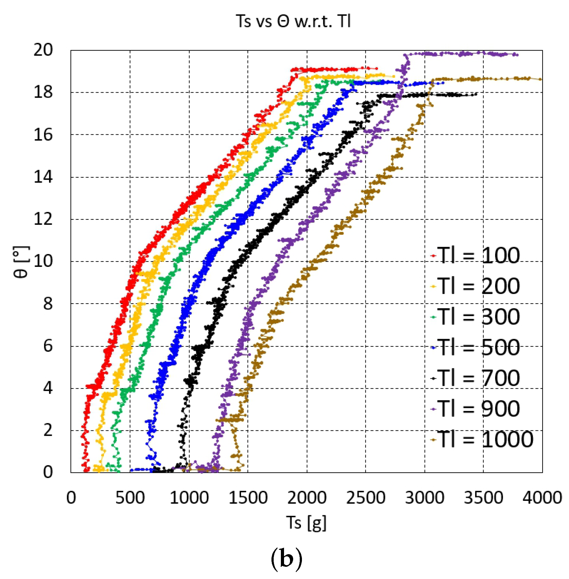
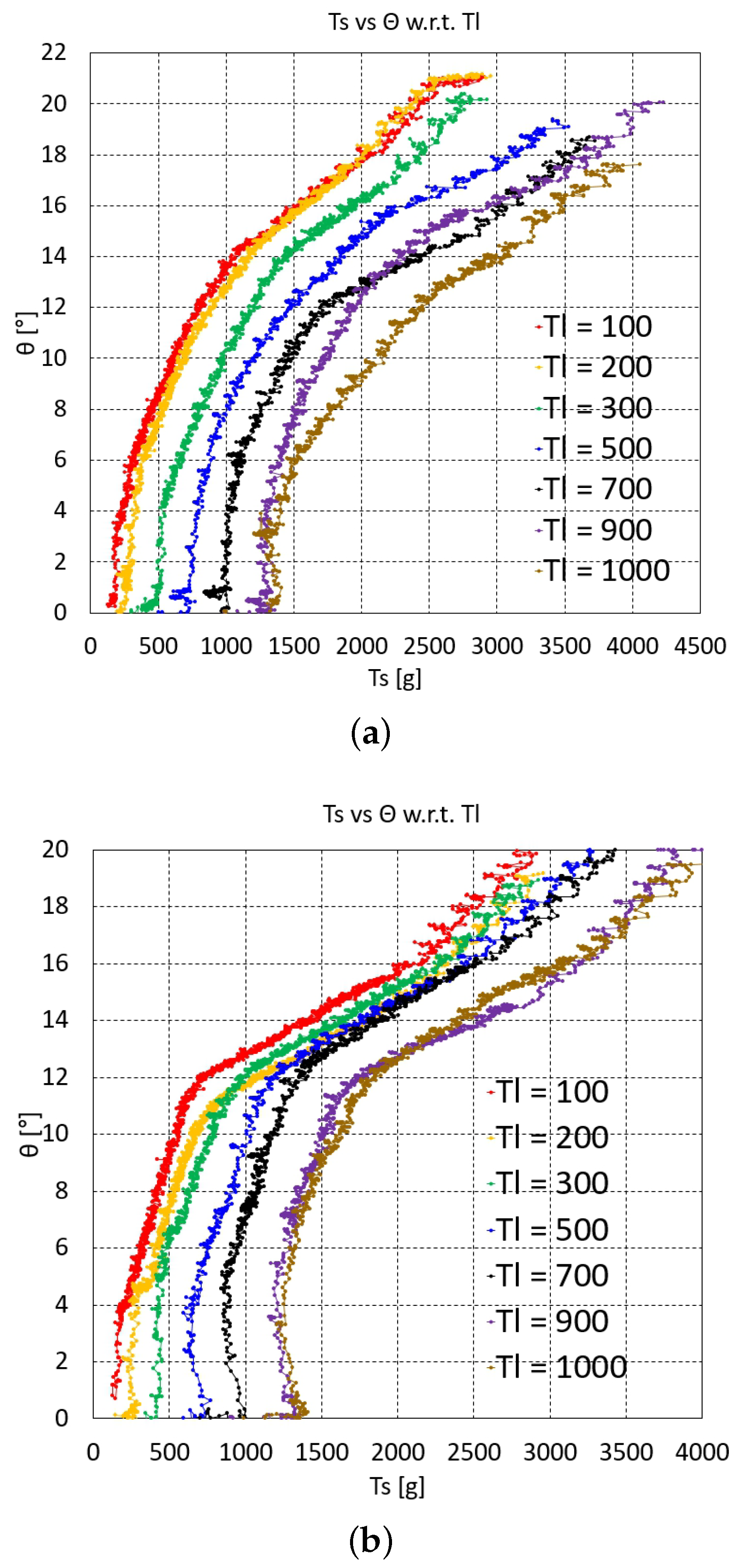
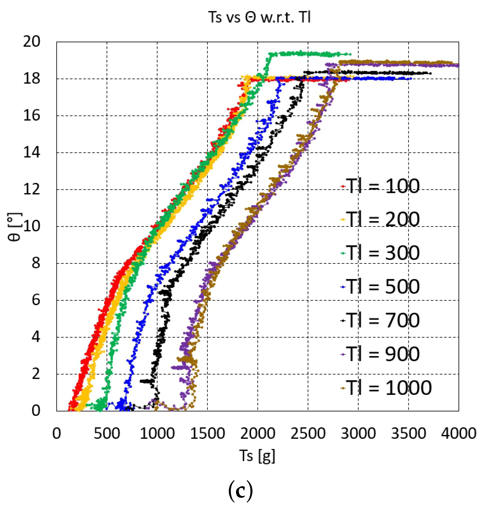
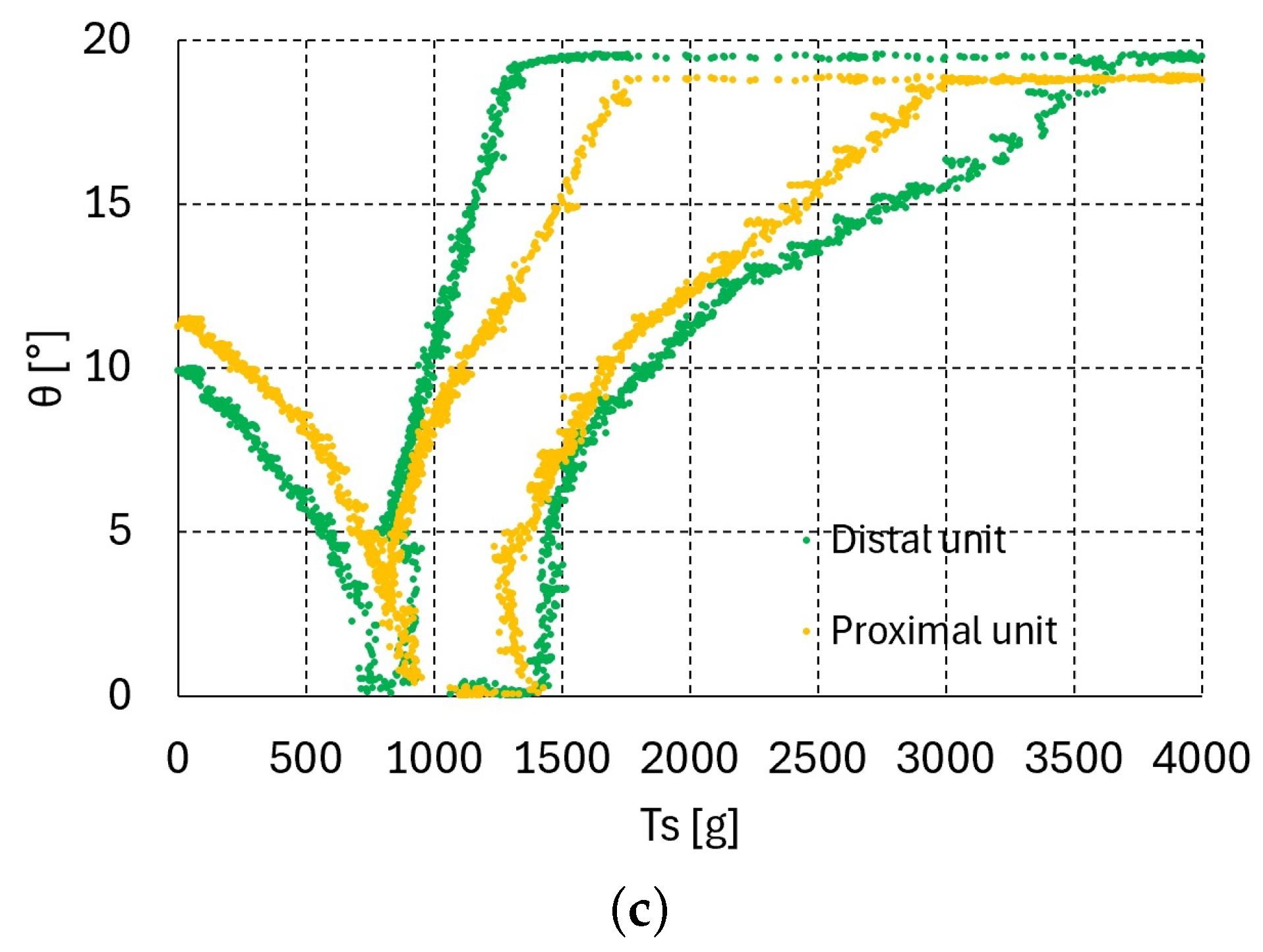
The graphs of vs. at each value of one, two, and three serially connected upper units are depicted in Figure 3, Figure 4a,b and Figure 5a–c, respectively. For two serially connected units, the graphs of the distal and proximal units are depicted in Figure 4a,b. For three serially connected units, the graphs of the distal, middle, and proximal units are shown in Figure 5a–c. In each of these vs. graphs, = 100, 200, 300, 500, 700, 900, and 1000 g plots are colored as red, orange, green, blue, black, purple, and brown, respectively.
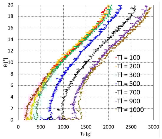
Figure 3.
vs. graphs of one upper unit.
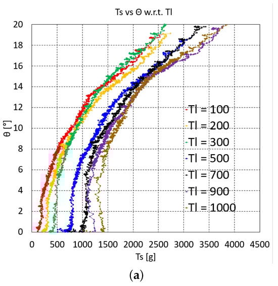
Figure 4.
vs. graphs of two serially connected upper units: (a) distal unit and (b) proximal unit.
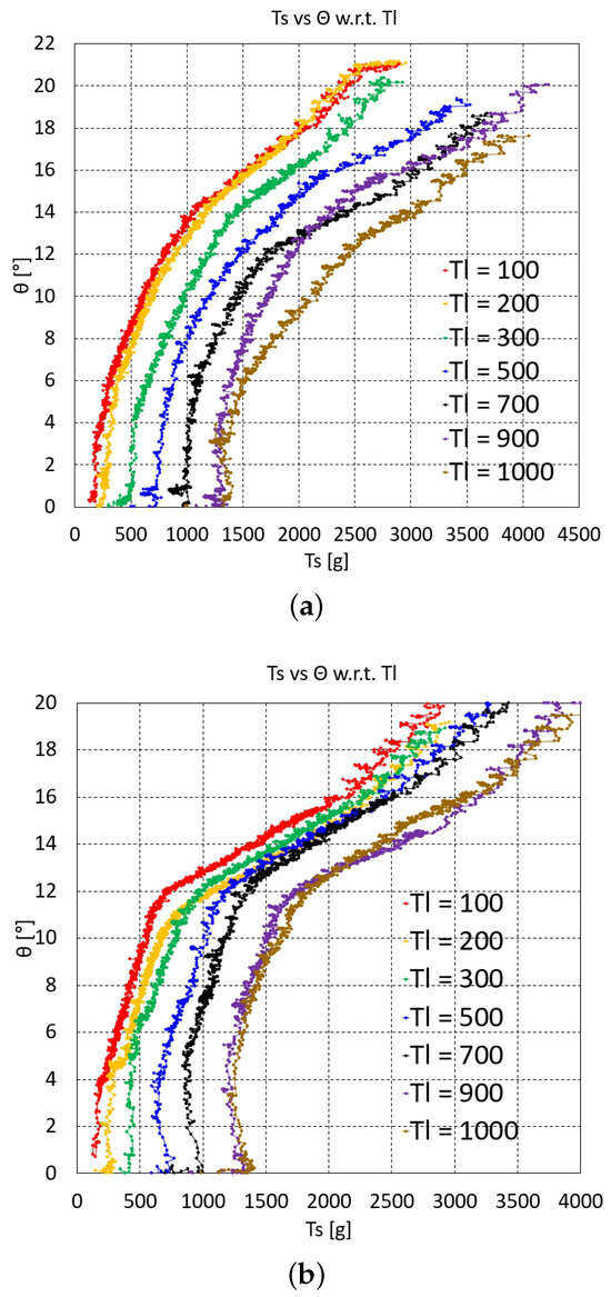
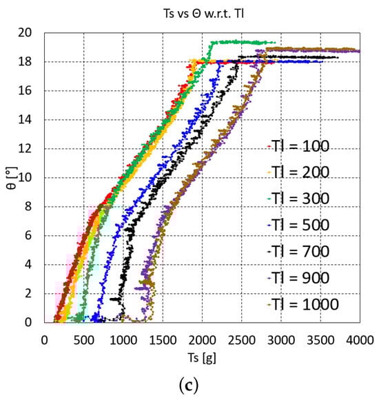
Figure 5.
vs. graphs of three serially connected upper units: (a) distal unit, (b) middle unit, and (c) proximal unit.
The overall characteristics of the graphs in Figure 3, Figure 4 and Figure 5c initially indicate that the graph gradient is rather large, gradually decreasing as increases and then increasing again. The initial steep gradient region in each graph is the initial Nitinol rod region prior to bending, where the value is almost zero and then suddenly increases at a specific value after bending occurs. This pre-bending region increases as increases. The pre-bending region is hard to control using the inverse statics. The actual bending occurring with and after bending of one, two, and three upper units are extracted from the graphs in Figure 3, Figure 4 and Figure 5c by graphical analysis and summarized in Table 1, Table 2 and Table 3, respectively. In Table 1, because – is linearly dependent on + , as described in Equation (2), if increases at the same bending angle, then the friction moment increases due to the increase in the normal force between the joint’s ball and socket.

Table 1.
Bending occurring and after bending in the graph of a single upper unit.
Table 2.
Bending occurring and after bending in the graph of two upper units.
Table 3.
Bending occurring and after bending in the graph of three upper units.
The graphs in Figure 3, Figure 4 and Figure 5c shift upward as the value decreases, which is natural consequence of force balance between with the same value. However, based on the experimental uncertainty, there are overlying graph regions in Figure 3, Figure 4a and Figure 5a–c, especially in the lower value graphs, which must be accounted for when performing the experiments. Figure 4b and Figure 5c contain flat graph region in the proximal unit graphs, which means that the proximal unit reaches the maximum bending angle before the distal and middle units reach their maximum bending.
For the interpolated inverse statics, each of the graphs in Figure 3, Figure 4 and Figure 5c must be curve-fitted with appropriate basis functions in a feasible bending angle range. In this study, third-order to fifth-order polynomials were selected for the curve fitting because they can fit all of the graphs in Figure 3, Figure 4 and Figure 5c with reasonable accuracy. However, because the middle unit graphs for three serially connected units (Figure 5b) have bilinear characteristics, they are fitted with two third-order to fifth-order polynomials. The average value of the polynomial fits for one, two, and three units are 0.9961, 0.9939, and 0.9914, respectively. With the polynomials at each value, the value can be determined at a specific value using linear interpolation. First, the (, ) pair can be used to determine whether or not the value is lower than the value after bending in Table 1, Table 2 and Table 3, which is done by linearly interpolating the value after bending in Table 1, Table 2 and Table 3. If the value is lower, then is not feasible. If it is higher, can be calculated by linearly interpolating the value using the fitting polynomials at = 100, 200, 300, 500, 700, 900, and 1000 g.
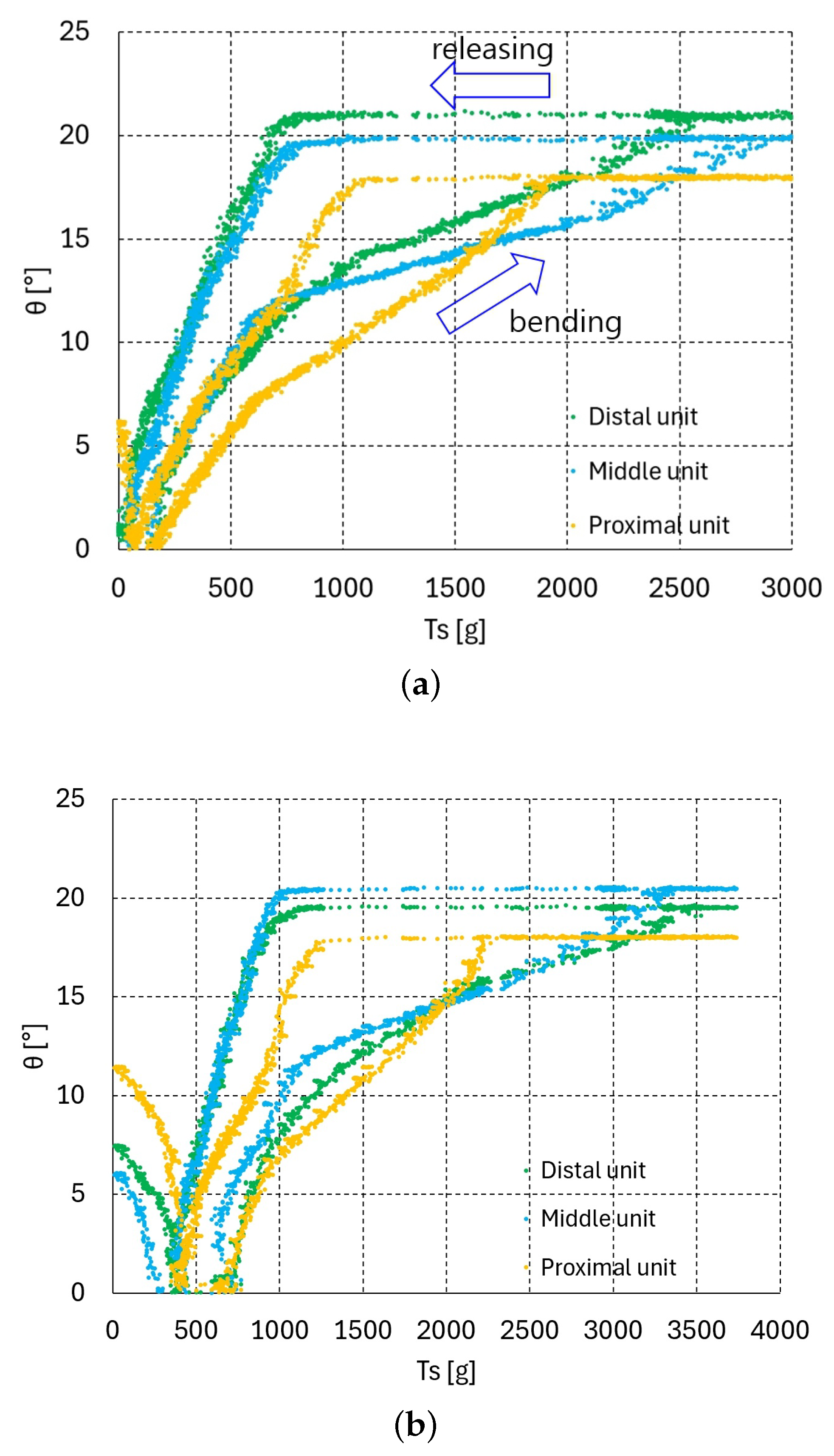
2.3.2. vs. Characteristics of One, Two, and Three Serially Connected Units in the Releasing Direction
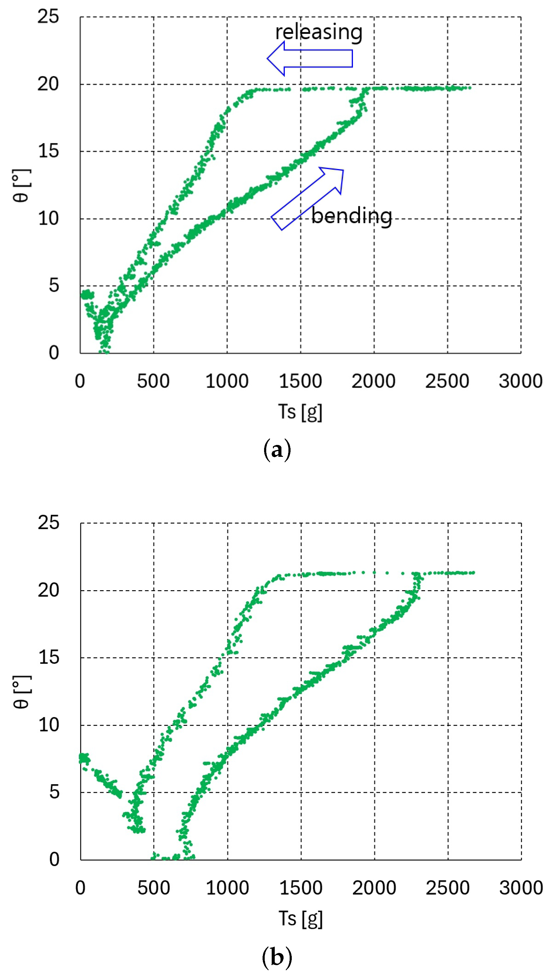
The graphs in Figure 3, Figure 4 and Figure 5c present the relationship between the bending angle and tendon tensions and for one, two, and three serially connected units. In the experiment for these graphs, the tension was increased until the maximum bending angle of 19.1° was reached at all of the upper units. If the tendon tension is released at the maximum bending angle = 19.1°, then the releasing vs. graphs differ from those in the bending direction graphs shown in Figure 3, Figure 4 and Figure 5c. Figure 6a–c, Figure 7a–c and Figure 8a–c present the bending–releasing vs. graphs at = 100, 500, 1000 g with one, two, and three serially connected upper units, respectively. The green, yellow, and sky-blue dots in Figure 6a, Figure 7 and Figure 8c present the graphs of the distal, proximal, and middle units, respectively. As can be seen in the graphs in Figure 6a, Figure 7 and Figure 8c, the bending and releasing graphs contain hysteresis. After the hysteresis, the releasing region presents almost linear characteristics regardless of whether or not the bending region has nonlinear characteristics. In addition, the slopes of the releasing regions in the distal and middle unit graphs in Figure 8a–c are almost identical. Note that the bending region in the bending and releasing graphs in Figure 6a, Figure 7 and Figure 8c is the same as in the graphs in Figure 3, Figure 4 and Figure 5c. The hysteresis in the bending–releasing graphs in Figure 6a, Figure 7 and Figure 8c is due to the initial releasing of and the static frictional moment between the ball–socket joint. Here, in Equation (2) is eliminated without changing bending angle, which is the inverse consequence of the bending procedure in Section 3. After hysteresis, and have a linear relationship in Equation (2) with ≈ 0, as presented in Figure 6a, Figure 7 and Figure 8c. However, the relationship between in Equation (2) and must be clarified to ensure its linearity, which is currently in progress by the authors.
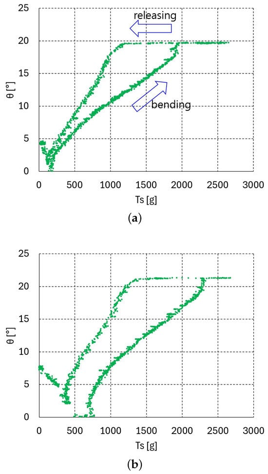

Figure 6.
vs. graphs of a single upper unit (bending–releasing) with = 100, 500, 1000 g: (a) = 100 g, (b) = 500 g, (c) = 1000 g.
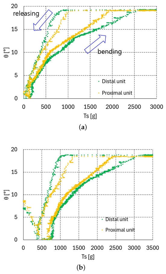
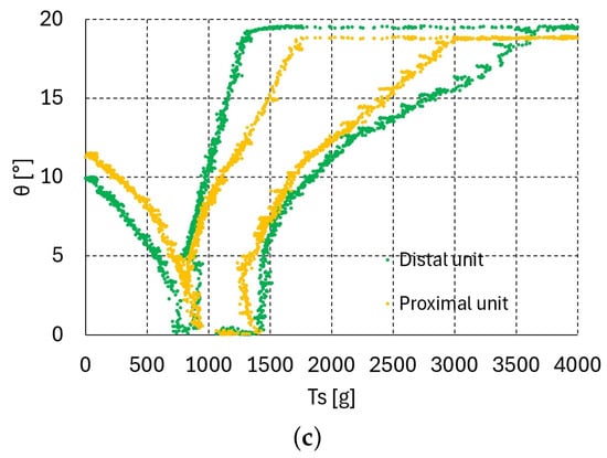
Figure 7.
vs. graphs of two upper units (bending–releasing) with = 100, 500, 1000 g: (a) = 100 g, (b) = 500 g, (c) = 1000 g.

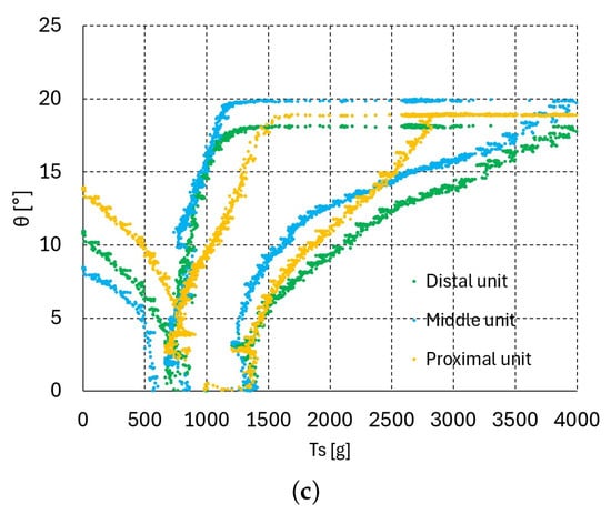
Figure 8.
vs. graphs of three upper units (bending–releasing) with = 100, 500, 1000 g: (a) = 100 g, (b) = 500 g, (c) = 1000 g.
3. Results and Discussions
3.1. Inverse Statics Validation Test Results
Inverse statics validation tests were performed to quantify the accuracy of the proposed interpolated inverse statics method. The value was set to 8, 12, and 16 degrees, while the value was set to 150, 400, and 800 g, representing intermediate values between the graphs in Figure 3, Figure 4 and Figure 5c. The value for each combination of and was calculated using the proposed interpolated inverse statics method. With the experimental setup shown in Figure 2, the and calculated values were applied and the resulting value was measured and recorded, with the results summarized in Table 4, Table 5, Table 6.
Table 4.
Inverse statics validation test results for a single upper unit (units: degrees, grams).
Table 5.
Inverse statics validation test results for two upper units (units: degrees, grams).
Table 6.
Inverse statics validation test results for three upper units (units: degrees, grams).
In Table 4, Table 5, Table 6, the column presents the value calculated using the proposed interpolated inverse statics, while the column presents the measured value when the calculated is applied to right-side tendon in Figure 2. The absolute error and % error columns in Table 4, Table 5, Table 6, present the value of (absolute measured ) and (absolute error/ × 100), respectively. The final rows in Table 3, Table 4 and Table 5 present the average absolute error and percentage error, with results of 0.3°, 2.7% with one upper unit, 0.7°, 6.6% with two upper units, and 0.6°, 5.3% with three upper units, respectively. These average percentage errors seem promising, even though relatively large errors are observed in Table 5 ( = 400 g condition) and Table 6 ((, ) = (8, 150) and (8, 800), respectively). There are also relatively large % errors in Table 5, such as 17% at = 8 degrees, Tl = 400 g, and = 886 g, which is thought to be a measurement error.
3.2. Ansys Dynamic Analysis Results for Unit Bending
To validate the experimental results, numerical simulations were conducted using Ansys version 2024 R1. The primary purpose of these simulations was not to guide the initial design process but rather to provide an independent numerical validation of the experimentally observed bending behavior. All simulation models were designed based on the actual diameters of the developed unit as depicted in Figure 1. Initially, we attempted to perform the simulations using the static structure module of Ansys; however, the results were not feasible because of the change in the unit’s status caused by the difference between the maximum static frictional moment and the static frictional moment. Because the static structure module does not support the input of the dynamic friction coefficient, we selected the Ansys motion module for dynamic simulation in subsequent analysis.
A tendon is structured as a yarn consisting of a continuous length of interlocking and twisted (spun) staple fibers. Consequently, the cross-sectional area of the tendon is challenging to measure accurately due to its irregular shape and imprecisely known packing density. For this reason, conventional definitions of density, stress, and tensile strength are not directly applicable. Instead, alternative metrics such as linear density and tenacity have been developed to characterize these properties. However, these material properties are seldom disclosed by tendon manufacturers, making it difficult to precisely determine the mechanical characteristics of the yarn. As a result, modeling tendons and incorporating their mechanical properties into finite element analysis (FEA) using Ansys remains a significant challenge.
To solve this and model the tendons in Ansys, the two tendon tension forces and were applied at the points in the upper unit where the tendons are connected. In this approach, a joint is created at the location where the tendon force is applied, with the joint’s coordinates positioned at the hole location of the lower unit. The tendon forces applied to the upper unit are configured to pass through the hole of the lower unit, simulating the actual pulling action of the tendons, as illustrated in Figure 9. To ensure that no deformation occurs in either unit and to allow for more efficient analysis, the stiffness characteristics of both units are modeled as rigid bodies. Standard Earth gravity is applied to all models in order to account for the effects of gravity.
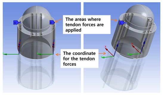
Figure 9.
The boundary conditions relating to force applied to the model (left: front view; right: isometric view).
Dynamic analyses were conducted for two cases, as described in Table 1: first with = 200 g and = 273 g, and second with = 300 g and = 405 g. The marker function within the Ansys motion module is used to track both the upper and lower units, and the resulting angle for each case is obtained as a simulation result. Initially, the tendon force is applied as the value to both tendons using a function expression and the joint vector load feature. After 1 s, an additional force corresponding to the difference between and is applied to the tendon with the value. A frictionless condition is applied to the contact area between the two units and the Nitinol wires. To replicate real experimental conditions, a fixed support condition is applied to the end surface of the lower unit.
The dynamic analysis results show that the angle after bending was 3.49° when = 200 g and = 273 g, while it was 3.93° when = 300 g and = 405 g. The angle for the case with = 200 g is depicted in Figure 10. A notable difference is observed between the experimental bending angle (2.5°) and the FEM result (3.49°) for the = 200 g case. While the friction at the ball–socket joint was modeled using the experimental friction coefficient, this discrepancy is primarily attributed to a necessary simplification in the model, namely, the application of a frictionless condition to the contact between the Nitinol wires and the unit holes. Unmodeled resistive forces from this wire–hole friction which are present in the physical setup likely account for the majority of the observed difference. This suggests that while the wire friction is difficult to measure, it is a non-negligible factor in the robot’s overall statics. Additionally, the stiffness of the wire may provide minor resistance as the upper unit tilts. Considering these factors, the simulation results align closely with the experimental findings summarized in Table 1, validating the accuracy of the experimental approach.
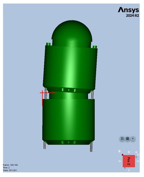
Figure 10.
Degree of tilting for two units in the FEM simulation results using Ansys.
3.3. Inverse Statics-Based Planar Path Planning for Three Serially Connected Units
With the developed interpolated inverse statics, a planar path planning method is proposed for three serially connected units. For the three serially connected units, , , , , and can be the dependent/independent variables. By the inverse statics, if two of these variables are selected as independent variables, then the other three variables can be calculated using the independent variables. Therefore, the control method for three serially connected units can be divided by which variables are the two independent variables, as described below.
- , →, ,
- , () →() →,
- , () →() →,
- , () →() →,
- , →, →
- , →, →
- , →, →
The two variables to the left-hand side of the arrow indicate the two independent variables, while the right-hand side variables are the dependent variables to be calculated based on the independent variables. In the proposed planar path planning method, and are selected as the two independent variables, as can be easily conjectured by the geometric configuration of the reference path and can be a tension representative variable, which together constitute the angle and tension variables in the search space. With these independent variables, the planar path planning method for three serially connected units is presented in Algorithm 1 below.
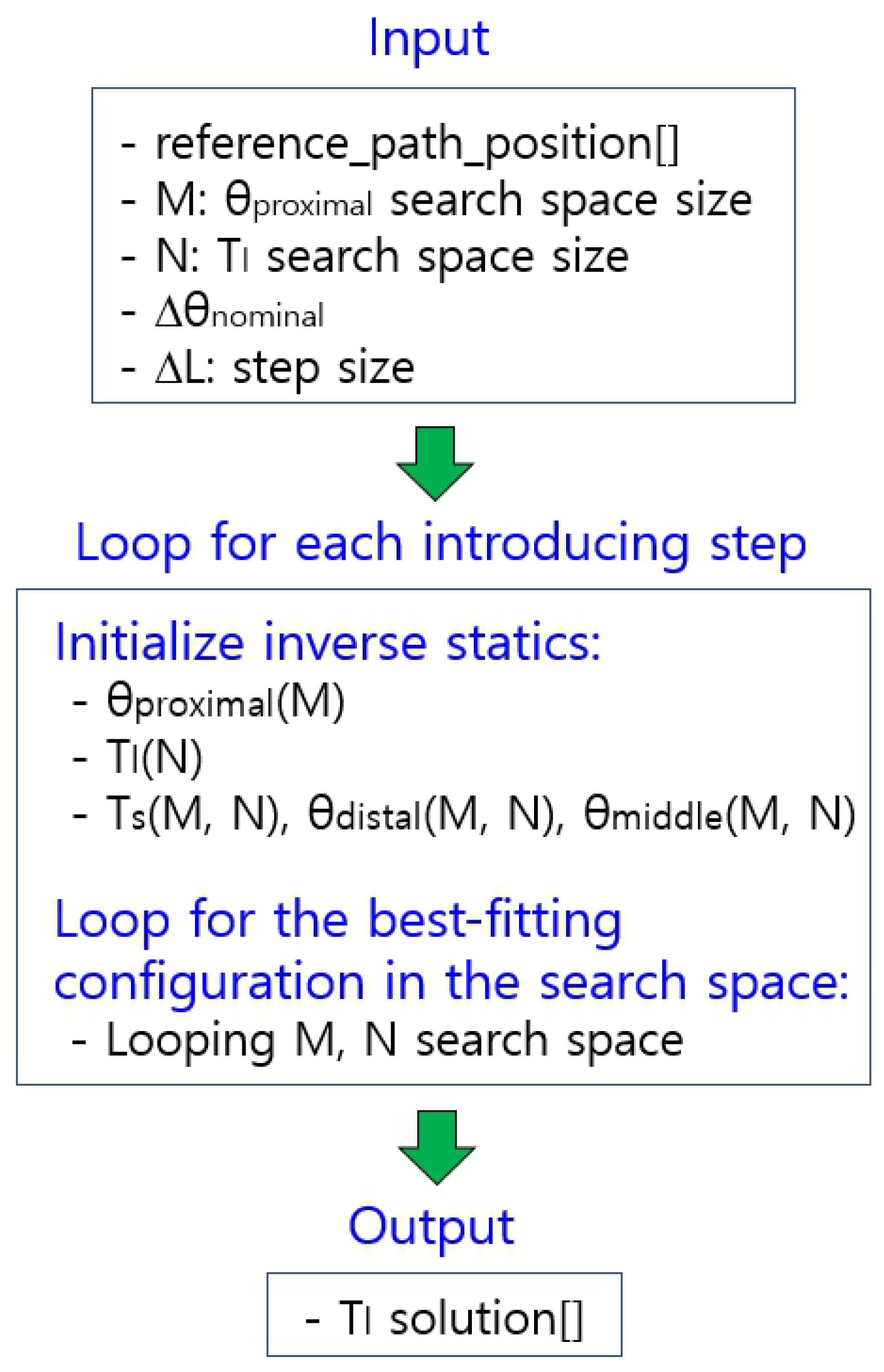
| Algorithm 1: Planar path planning for three serially connected units |
 |
In Algorithm 1, the input data consist of the reference path position, M, N, , and , while the output data consist of _solution and _solution at each introducing step. Here, M and N are the search space sizes of and , respectively. In line 1 of Algorithm 1, is calculated with Calculate_nominal_() by dividing the reference path into three equally-distanced linear segments and calculating the angle of the first linear segment with respect to the x axis. Then, and are calculated. The total number of introducing steps for the serially connected units is calculated in line 2.
Next, for each introducing step of the serially connected units, we first initialize all of the needed columns and the matrix with the interpolated inverse statics in line 4. Here, is the column of size M calculated by and , with ascending order as the index of column increases; is calculated similarly. The matrix has size , in which can be calculated with and using the interpolated inverse statics. Finally, and can be calculated using the interpolated inverse statics with and the matrix .
When initialization of the columns and matrix is complete, the minimum_position _difference is set to 1000. Then, we loop through M and N to find the best-fitting configuration in lines 5–10. In the “for” loop, the robot_configuration_position[] with , , and is calculated at each i and j index, and the corresponding reference path configuration is also calculated. With these two positions, the position_difference can be calculated. If the position_difference is smaller than the mininim_position_difference, we set the mininim_position_difference to position_difference and set _solution(step) and _solution(step) values to and , respectively. When all the inner and outer loops finish, _solution(total_introducing_steps) and _solution (total_introducing_steps) are returned in line 12.
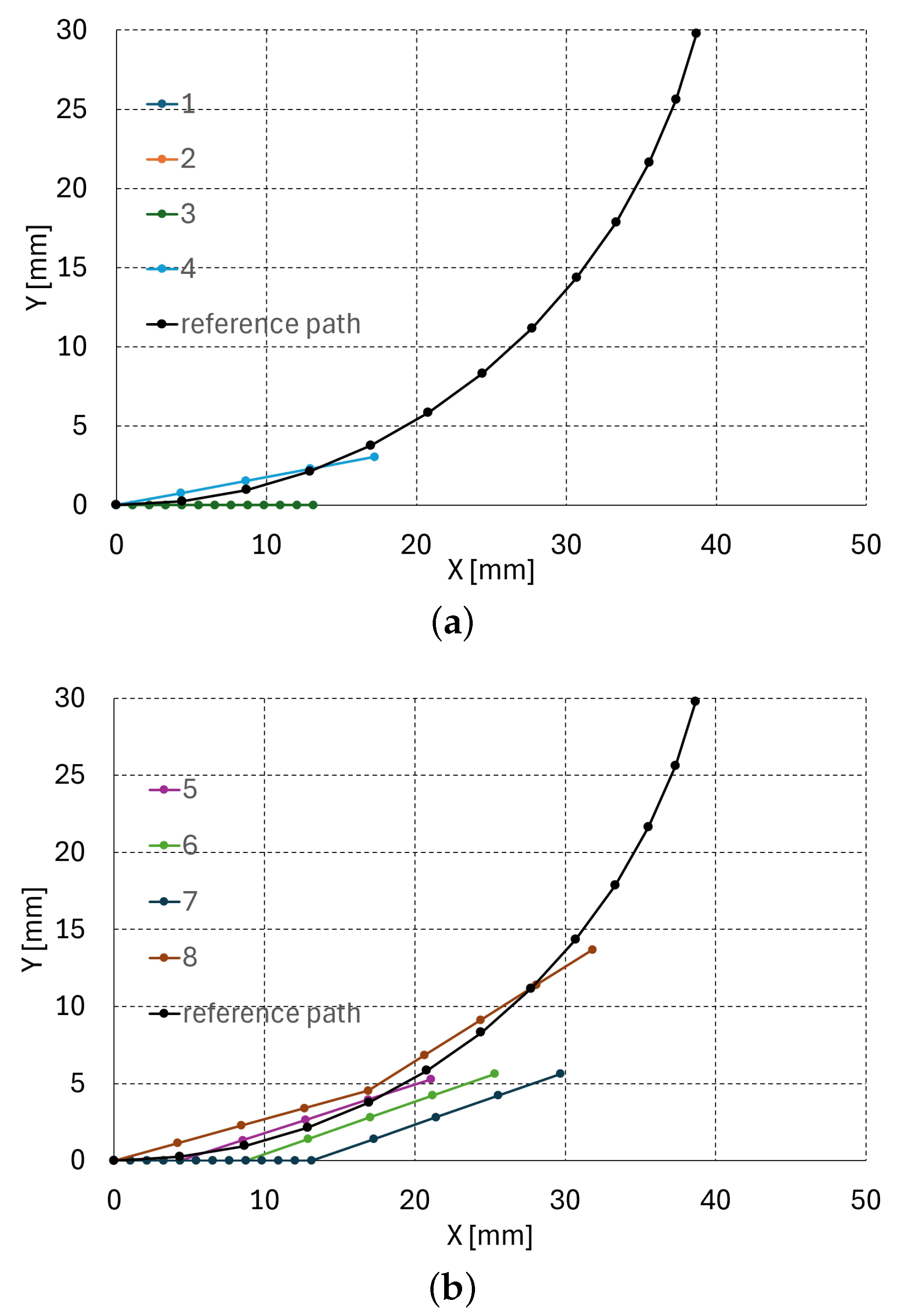
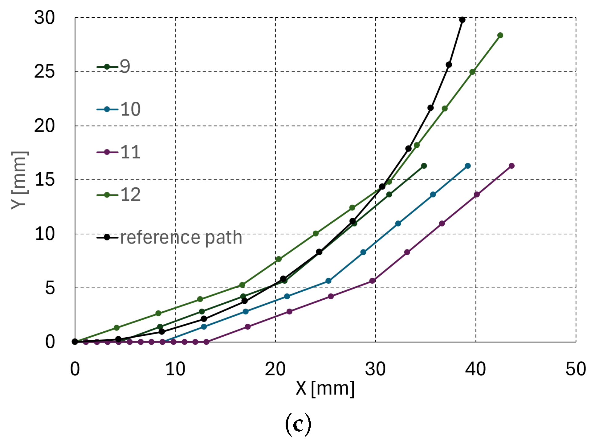
Using Algorithm 1, a planar path planning simulation was performed using the arc reference path, as depicted in Figure 11a–c. The overall flowchart of Algorithm 1 is depicted in Figure 12.
Figure 11.
Planar path planning simulation result with an arc reference path (R = 40 mm, = 82.3°): (a) steps 1–4, (b) steps 5–8, (c) steps 9–12.
Figure 12.
Overall flowchart of Algorithm 1.
In Figure 11a–c, the radius and angle of the reference arc are 40 mm and 82.3°, respectively. The three serially connected units are introduced at a quarter of the unit’s length (17.5/4 = 4.375 mm) increment, which constitutes twelve total steps for full introduction. Figure 11a–c presents the planar path planning result of steps 1–4, 5–8, and 9–12, respectively.
In the simulation, M, N, and were set to 16, 16, and 10°, respectively. Note that the line segment between the dots in Figure 11a–c is 4.375 mm in length. The robot configuration seems to have the best fit to the reference path at steps 4, 8, and 12, since at these steps the joint is at the origin to be deflected. At the other steps, the body of the unit is at the origin, meaning that the path planner just pushes the robot, as presented at steps 1–3, 5–7, and 9–11 in Figure 11a–c, respectively. Table 7 summarizes the planar path planning results. In Table 7, the first column presents the step number, the upper three columns are the distal, middle, and proximal angle, and the lower three columns are , , and the average position difference between the reference path and the configuration of the three units, respectively. The position difference is the largest at steps 10 and 11, which is evident in Figure 11c. Here, (, ) at each step in Table 7 is rather diverse depending on the best fitting configuration of the serially connected units. The large tracking error of 19.77 mm at step 11 in Table 7 is because there are four points in a unit in Figure 11, and the continuum robot can only be controlled at the joint in every four points (in Figure 11c, there is only translational movement at step 9–11; at step 12, the robot can be controlled because the joint coincides with the origin and the robot can be controlled at the joint.
Table 7.
Planar path planning simulation result with an arc reference path (R = 40 mm, = 82.3°).
4. Conclusions
In this work, we have demonstrated a practical data-driven inverse statics-based framework. Planar inverse statics for a tendon-driven discrete continuum robot unit with a ball–socket joint and superelastic Nitinol rods is proposed for one, two, and three serially connected units using an experiment-based interpolation method. The 2D bending procedure of the unit using two superelastic Nitinol rods under tendon tensions and is described. These operational conditions are categorized into static, quasi-static, and dynamic states, excluding the phase when the Nitinol rods begin to bend. After dynamic status is attained, when bending of the Nitinol rod begins, the static equilibrium status is again reached by the deflected Nitinol rod, as described by Equation (2). Accordingly, the inverse statics of the tendon-driven discrete continuum robot unit exhibits nonlinear characteristics.
The inverse statics results for one, two, and three serially connected units are provided in Table 1, Table 2, Table 3, Table 4, Table 5 and Table 6, and Figure 3, Figure 4 and Figure 5c. The results indicate the existence of nonlinear characteristics; specifically, the stepwise bending angle increases in the lower value region. This region corresponds to the region in which Equation (1) can be applied. A hysteresis effect is also observed during tendon pulling and releasing, as described in Figure 6a, Figure 7 and Figure 8c. This hysteresis is thought to stem from the changes between the bending and unfolding directions during interactive moment (i.e., the contact frictional moment and deflectional moment).
The validity of the proposed interpolated inverse statics method was confirmed through experiments, wherein eighteen (, ) pairs were selected and values calculated for each pair using the proposed method. The and calculated values were applied to the unit’s tendons, then the resulting bending angles were measured. The average percentage error between the reference and measured for one, two, and three serially connected units were found to be 2.7, 6.6, and 5.3%, respectively. This error comprises both experiment-based errors (measurement uncertainty, ball–socket joint contact condition uncertainty) and modeling errors (polynomial fitting error, interpolation error). These errors should be considered as the uncertainty in statics-based unit control.
In addition, the results of our FEM simulations in Ansys (Figure 10) are consistent with the results in Table 1, with a bending angle of approximately 3.49 degrees under the 200 g and 270 g condition in Table 1. The discrepancy between the simulation and experimental results under these conditions is 0.99 degrees.
Based on the proposed interpolated inverse statics, a planar path planning method is proposed for three serially connected units, with and selected as the independent search space parameters. With these parameters, the dependent parameters , , and can be calculated. The (, ) pair shows the best fit to the reference path, and as such was selected as the path planning solution. The proposed planar path planning method was verified through simulations using the arc reference path, with average position differences of 6.29 mm of in Table 7.
The proposed planar inverse statics approach was constructed with only one, two, and three serially connected units. However, real clinical situations require more than three units. For trans-oral surgery assisted by a continuum robot with the designed unit, more than ten units would be needed. Therefore, multi-section inverse statics must be devised with the tendon tension propagation model along the sections, with three serially connected units comprising a section. In addition, the developed unit in Figure 1 is initially designed for 3D bending capability; however, in this study the developed inverse statics are planar in nature. If the driver of the trans-oral assisting continuum robot can axially rotate the continuum robot, then the missing degrees of freedom can be supplemented. To accommodate various driver mechanisms, 3D inverse statics must be developed based on the foundation of the developed planar inverse statics. The proposed path planning algorithm with three serially connected units has only been verified by simulation; thus, further experiments must be carried out in order to verify the simulation results, which is a focus of our future work. Moreover, although the proposed method has been experimentally validated, clinical translation requires further testing in realistic surgical environments, including robustness under tissue interaction and dynamic force compensation. Future work will involve developing a high-fidelity FEA model early in the design process in order to guide the optimization of key design parameters such as joint geometry and material properties prior to fabrication. These aspects will also be addressed in future work.
Author Contributions
Conceptualization and design, Y.-J.K. and D.W.; methodology, Y.-J.K. and D.W.; data collection, Y.-J.K. and D.W.; analysis and interpretation, Y.-J.K. and D.W.; writing the article, Y.-J.K. and D.W.; critical revision, Y.-J.K. and D.W.; final approval of the article, Y.-J.K. and D.W. All authors have read and agreed to the published version of the manuscript.
Funding
This research was supported by a grant (RS-2021-NR061860) and (No. 2021R1C1C2006999) from the National Research Foundation of Korea (NRF), funded by the Ministry of Science and ICT (MSIT), Republic of Korea.
Data Availability Statement
The data that support the findings of this study are available from the corresponding author upon reasonable request. The data are not publicly available due to their volume and the absence of a public repository submission.
Conflicts of Interest
The authors declare no conflicts of interest.
References
- Burgner-Kahrs, J.; Rucker, D.C.; Choset, H. Continuum Robots for Medical Applications: A Survey. IEEE Trans. Robot. 2015, 31, 1261–1280. [Google Scholar] [CrossRef]
- Wang, M.; Dong, X.; Ba, W.; Mohammad, A.; Axinte, D.; Norton, A. Design, modelling and validation of a novel extra slender continuum robot for in-situ inspection and repair in aeroengine. Robot. -Comput. -Integr. Manuf. 2021, 67, 102054. [Google Scholar] [CrossRef]
- Yang, Z.; Yang, L.; Sun, Y.; Chen, X. Comprehensive kinetostatic modeling and morphology characterization of cable-driven continuum robots for in-situ aero-engine maintenance. Front. Mech. Eng. 2023, 18, 40. [Google Scholar] [CrossRef]
- Li, G.; Yu, J.; Dong, D.; Pan, J.; Wu, H.; Cao, S.; Pei, X.; Huang, X.; Yi, J. Systematic Design of a 3-DOF Dual-Segment Continuum Robot for In Situ Maintenance in Nuclear Power Plants. Machines 2022, 10, 596. [Google Scholar] [CrossRef]
- Hussain, T.; Lang, S.; Haßkamp, P.; Holtmann, L.; Höing, B.; Mattheis, S. The Flex robotic system compared to transoral laser microsurgery for the resection of supraglottic carcinomas: First results and preliminary oncologic outcomes. Eur. Arch. Otorhinolaryngol. 2020, 277, 917–924. [Google Scholar] [CrossRef] [PubMed]
- Yang, W.; Cao, Y.; Wang, S.; Liu, Z.; Cheng, H.; Xie, L. Development of a continuum manipulator with variable bending length and piecewise stiffness for transoral laryngeal surgery. Int. J. CARS 2024, 19, 1809–1820. [Google Scholar] [CrossRef] [PubMed]
- Feng, F.; Zhou, Y.; Hong, W.; Li, K.; Xie, L. Development and experiments of a continuum robotic system for transoral laryngeal surgery. Int. J. CARS 2022, 17, 497–505. [Google Scholar] [CrossRef] [PubMed]
- Zhang, D.; Sun, Y.; Lueth, T.C. Design of a novel tendon-driven manipulator structure based on monolithic compliant rolling-contact joint for minimally invasive surgery. Int. J. CARS 2021, 16, 1615–1625. [Google Scholar] [CrossRef] [PubMed]
- Amanov, E.; Nguyen, T.-D.; Burgner-Kahrs, J. Tendon-driven continuum robots with extensible sections—A model-based evaluation of path-following motions. Int. J. Robot. Res. 2021, 40, 7–23. [Google Scholar] [CrossRef]
- Rucker, D.C.; Jones, B.A.; Webster, R.J. A Geometrically Exact Model for Externally Loaded Concentric-Tube Continuum Robot. IEEE Trans. Robot. 2010, 26, 769–780. [Google Scholar] [CrossRef] [PubMed]
- Russo, M.; Sadati, S.M.H.; Dong, X.; Mohammad, A.; Walker, I.D.; Bergeles, C.; Xu, K.; Axinte, D.A. Continuum Robots: An Overview. Adv. Intell. Syst. 2023, 5, 2200367. [Google Scholar] [CrossRef]
- Auyang, E.D.; Santos, B.F.; Enter, D.H.; Hungness, E.S.; Soper, N.J. Natural orifice translumenal endoscopic surgery (NOTES®): A technical review. Surg. Endosc. 2011, 25, 3135–3148. [Google Scholar] [CrossRef]
- Sun, Y.; Lueth, T.C. Enhancing Torsional Stiffness of Continuum Robots Using 3-D Topology Optimized Flexure Joints. IEEE/ASME Trans. Mechatronics 2023, 28, 1844–1852. [Google Scholar] [CrossRef]
- Childs, J.A.; Rucker, C. Leveraging geometry to enable high-strength continuum robots. Front. Robot. 2021, 8, 629871. [Google Scholar] [CrossRef] [PubMed]
- Kim, Y.-J.; Choi, J.; Choi, J.; Moon, Y. Genetic Algorithm-based Discrete Continuum Robot Design Methodology for Transoral Slave Robotic System. Int. J. Control Autom. Syst. 2022, 20, 3361–3371. [Google Scholar] [CrossRef]
- Jones, B.A.; Walker, I.D. Practical Kinematics for Real-Time Implementation of Continuum Robots. IEEE Trans. Robot. 2006, 22, 1087–1099. [Google Scholar] [CrossRef]
- Kim, Y.-J.; Moon, Y.; Choi, J.; Wi, D. Planar interpolated inverse statics for a tendon-driven discrete continuum robot unit with a ball socket joint and superelastic Nitinol rods. In Proceedings of the 24th International Conference on Control, Automation and Systems (ICCAS), Jeju, Republic of Korea, 29 October–1 November 2024; pp. 1311–1312. [Google Scholar]


Disclaimer/Publisher’s Note: The statements, opinions and data contained in all publications are solely those of the individual author(s) and contributor(s) and not of MDPI and/or the editor(s). MDPI and/or the editor(s) disclaim responsibility for any injury to people or property resulting from any ideas, methods, instructions or products referred to in the content. |
© 2025 by the authors. Licensee MDPI, Basel, Switzerland. This article is an open access article distributed under the terms and conditions of the Creative Commons Attribution (CC BY) license (https://creativecommons.org/licenses/by/4.0/).