A Methodology to Characterize an Optimal Robotic Manipulator Using PSO and ML Algorithms for Selective and Site-Specific Spraying Tasks in Vineyards

Abstract

This paper presents an improved methodology for characterizing task-oriented optimal manipulator configuration, tested on a case study of selective spraying in vineyards. It compares the current approach for optimizing manipulator configurations, which relies on simulation and optimization algorithms, with an improved methodology that integrates machine learning models to enhance the optimization process. The simulation tool was developed using the Gazebo simulator and ROS software to evaluate potential robotic configurations within a simulated vineyard. Particle Swarm Optimization (PSO) was employed as the optimization algorithm in a finite solution space, with the performance measure based on maximizing the Manipulability Index of manipulator configurations reaching all targets. In the proposed methodology, XGBoost models were used to replace the simulation stage in the process and predict the manipulator’s ability to reach the target positions in the spraying task. This prediction served as decision support in selecting which configurations should be tested in the simulation, thereby reducing computational time. The integration of machine learning models in the proposed methodology resulted in an average runtime reduction of 59% while maintaining an average manipulability index score in comparison to the original approach, which did not include the XGBoost model. This methodology demonstrates significant enhancements in optimizing robot configuration for a specific task and shows strong potential for broader applications across various industries.

1. Introduction

In this study, we present a novel methodology to characterize an optimal robot designed for selective spraying in table grape vineyards. The vineyard features a Y-shaped trellising system (Figure 1), which forms a Y-shaped structure to support the grapevines. The spraying targets are the fruit clusters. Gibberellin, a plant hormone commonly used in grape production, was chosen as the spraying agent. It is applied at various concentrations during fruit growth to enhance fruit size, yield, and quality [1]. Currently, this task is performed manually, either by hand spraying directly onto the fruit clusters or by dipping the clusters into a solution container. Both methods are time consuming, labor intensive, imprecise, and often lead to excessive application and material waste [2]. Employing robotic systems can facilitate faster and more accurate delivery of spraying materials. The spraying process involves applying large quantities of chemicals, which can have significant environmental impacts and potential health hazards [3]. Achieving a consistent deposition rate and applying the optimal amount of material to each target are critical goals in spraying tasks. However, plants often receive either overdoses or underdoses of chemicals [4]. Advances in computer vision and artificial intelligence integrated into robotic sprayers promise to enable precise and accurate selective spraying [5]. Utilizing robots for this task can reduce environmental harm and operational costs while ensuring materials are delivered exactly where needed.

This study proposes an improved methodology for characterizing optimal manipulator configurations for a specific task by developing a new concept and integrating machine learning algorithms into the optimization process. This new methodology can enhance performance, reduce costs, and increase accessibility and widespread use. The focus of this study is on the optimization of task-oriented manipulators.

1.1. Robot Optimization

Robots have been developed to perform tasks that are repetitive, dull, strenuous, or hazardous, offering significant advantages in efficiency and safety [6]. In agriculture, robots have the potential to greatly enhance the efficiency and precision of tasks such as weeding, harvesting, and spraying. Despite their successful implementation in industrial settings, the adoption of robots in agriculture has been limited, primarily due to the complexity and variability of agricultural environments. Industrial environments are more predictable and uniform, while agriculture faces a variety of challenges, such as weather conditions, unstructured terrain, and plants or produce that vary in color, size, and shape, all of which can be easily damaged during handling [6,7]. Despite decades of research, commercial applications of agricultural robots remain limited, mainly due to the high cost of robots, maintenance requirements, and incomplete performance [8]. Nevertheless, there is an economic incentive to use robots and automation in agriculture, particularly in countries with high labor costs and manpower shortages.

In previous years, several approaches have been proposed to optimize robot parameters based on different performance criteria. Zhou and Bai [9] presented in their study a method for optimizing a robotic arm to minimize the weight of the robot with constraints on kinematics performance, dynamic requirements, and structural strength. The kinematic performance of the robot was indexed by the global conditioning index (GCI). The optimization method was implemented by using five modules, including a computer-aided design (CAD), a kinematic and dynamic simulation, a finite element analysis system module, and a complex optimization method. Xiao et al. [10] focused on optimizing the total mass but also the manipulability of a robotic arm based on non-dominated sorting genetic algorithm II (NSGA-II) and Pareto fronts. The study engaged in optimizing the structure of the existing Universal Robot (UR) with a payload of 5 kg.

Meir et al. [11] conducted a comparative study of various optimization algorithms applied to the problem of optimal robot design, including Particle Swarm Optimization (PSO), the Artificial Bee Colony (ABC), Evolution Strategies (ES), the Whale Optimization Algorithm (WOA), the Genetic Algorithm (GA), Simulated Annealing (SA), and Sequential Least Squares Programming (SLSQP). Their findings indicated that PSO exhibited a superior convergence rate, fitness performance, and computational efficiency. Furthermore, they introduced a novel optimization framework utilizing PSO to adapt robotic arm kinematics for precise path following based on trajectories demonstrated by human experts. This optimization targeted the enhancement of robot performance for specific tasks by refining design parameters informed by human motion data. The PSO algorithm effectively managed the complex search space, achieving reduced computational overhead while preserving solution accuracy [11]. Similarly, PSO has been employed in the optimization of parallel manipulators. Shirazi et al. [12] formulated an optimization problem involving three performance metrics: a reachable workspace, condition number (serving as an indicator of error amplification in joint space), and structural stiffness, combined into a cost function. The design variables comprised five geometric parameters constrained within specified bounds. To mitigate velocity stagnation issues inherent in PSO, the authors incorporated random mutation into the algorithm. Farooq et al. [13] also utilized PSO to optimize three criteria—the conditioning index, workspace volume, and global conditioning index—by constructing a weighted multi-objective summation function.

1.2. Robotic Simulation

Robotic simulation constitutes a critical tool for the efficient development, testing, and validation of robotic designs, operational strategies, and software systems [14]. These simulation platforms are important in the design phase [15], facilitating the evaluation, debugging, and optimization of sensing mechanisms, trajectory planning, and control algorithms. Moreover, simulations enable comprehensive assessments across diverse environmental conditions, thereby supporting the identification of potential system deficiencies and informing iterative improvements [16].

Takaya et al. [17] introduced a simulated environment for mobile robots utilizing Robot Operating System (ROS) and Gazebo robotic software tools. Within this framework, the Universal Robotic Description Format (URDF), an XML file format standardized in ROS, is employed to represent the various elements of a robot model, including sensors, joints, and links of the robot. It demonstrates that once robot models are accurately created in Gazebo, the associated control code can be directly deployed to real robots. The research explored autonomous navigation tasks and 3D-mapping simulations conducted within the proposed environment, highlighting the strong alignment between simulation and experimental results. The findings underline the effectiveness of this developed simulation framework in enhancing the reliability and efficiency of robotic systems. Zhibao et al. [18] focused on developing a robotic simulation system by integrating the USARSim and RCS (Real-time Control System) software libraries. This combined system leverages USARSim’s capabilities and RCS libraries to create a realistic environment with sensors, robot configurations, and an RCS-based controller. A control system for a four-wheeled robot was tested in the simulation, validating its essential processes in perception, trajectory planning, and adapted tracking. The analysis of experimental data demonstrated optimal performance in terms of route execution, offering tracking tools and corresponding data. Huang et al. [18] conducted a study using simulation tools to analyze and compare a robotic arm’s responses under different algorithms and different target poses. The simulation model consists of three parts: (1) describing the robot’s physical characteristics and configuration in URDF and SRDT files; (2) handling the parameter input, model loading, and result retrieval; and (3) simplifying system operation with options for algorithm selection and simulation initialization. Gazebo software was selected for its physical engine and file compatibility. The study’s effectiveness led to a suggestion of future machine learning algorithm integration for accurate and faster route planning.

1.3. Machine Learning in Robotics

Machine learning (ML) and deep learning (DL) algorithms have had a significant impact on robotics, leading to advancements in various areas such as reinforcement learning for robot control, computer vision for robotic manipulation and grasping, and for mobile robot navigation. However, learning-based solutions come with the drawbacks of unpredictability and high computational complexity [19]. One of the most general-purpose applications of learning techniques in robotics is to approximate a function’s value using training samples. This approach can be used to map actions to corresponding changes in state, changes in state to actions, or forces to motions. In cases where these equations are impossible to produce acceptable accuracy due to complex environments, approximating functions from sample observations can yield significantly improved accuracy. These function-approximating models can also excel in classification tasks such as identifying objects or determining the best grasping approach or planning strategy for a given situation [20]. Yue et al. utilized predictive ML models in the realm of manipulator stability research [21]. This research addresses the limitations of traditional robot control methods in meeting the demands for flexibility and adaptability in modern applications like intelligent manufacturing. The study proposes a predictive method using Long Short-Term Memory (LSTM) and Extreme Gradient Boosting (XGBoost) to assess manipulator stability. The approach enables accurate predictions of stability levels based on command parameters, with a minimum Mean Absolute Error of 0.0024, indicating the model’s potential to enhance the precision and reliability of robotic manipulators in dynamic environments. Lin et al.’s study [22] enhances an artificial potential field (APF) method by integrating decision tree principles, which are commonly used for classification. The research proposes an improved APF model that allows for accurate, real-time behavior recognition and swift decision-making in complex indoor environments. The enhanced model results demonstrate a 50% reduction in planning time and a 43.3% improvement in path smoothness compared to the traditional APF method. Yoo et al. [23] introduced an advanced Predictive Maintenance (PdM) method aimed at forecasting failures in wafer transfer robots within semiconductor manufacturing, where minimizing downtime and maintenance costs is crucial. Features between normal and error states were used to train an artificial neural network model, which successfully predicted failures with a 97% classification accuracy.

Lenz et al. [24] utilized a deep learning algorithm to identify optimal grasps for objects using RGB images. The network assesses multiple potential grasps for an object and selects the most successful one without any prior knowledge of the object’s geometry. Testing on Baxter and Personal Robot 2 (PR2) resulted in successful grasps 84% and 89% of the time, respectively. Wu et al. [25] used a generative model to anticipate outcomes from physics simulations, while Watter et al. [26] utilized a generative model to model nonlinear dynamics in simple physical systems and control them. It is apparent that various learning model structures can be applied to a wide range of problems in the field of robotics. However, the model architecture, learning formulation, and training strategy must be tailored to suit the specific robotic problem, task, and environment being investigated.

1.4. Agricultural Robotics

Recent advances in agriculture have focused on improving spraying efficiency and reducing pesticide usage through robotics and sensor-based systems. Oberti et al. [27] conducted a study on a robot system that can perform automatic selective spraying in vineyards. The robot system used in the study was based on a designed robot for crop applications with six DOF, a syringe for precise spraying, pesticide liquids, and a disease-sensing system that conducted multi-spectral imaging, all integrated through an electronic and communication-based architecture, which was implemented by ROS and a modular user interface to communicate with the robot system. The results showed that robotic selective spraying achieved a reduction of 64% of the amount of material compared to conventional homogeneous spraying, covering 95% of the infected plant surfaces. The issue of spraying pesticides in vineyards and orchards was examined in a study by Wandkar et al. [28]. Farmers use air-blast sprayers, which can result in material loss due to drift during spraying and inefficiency. The study showed that variable-rate sprayers reduced the use of pesticides by 30–80% compared to traditional methods of spraying.

Previous research has focused on enhancing spraying efficiency through the integration of sensors and vision systems; however, these approaches typically utilize pre-existing robotic platforms without optimizing the manipulator design. Optimizing the manipulator can significantly improve precision, minimize redundant movements, and ensure effective functionality within complex agricultural environments. In the absence of such optimization, even advanced sensing and spraying techniques may be constrained by limited workspace accessibility and suboptimal kinematic performance.

2. Methods

2.1. Robot Manipulator Description

Serial manipulators were selected as the kinematic architecture for the optimal manipulator design. A serial manipulator comprises a fixed base, a sequence of links interconnected by joints, and an end-effector. All actuated joints possess a single degree of freedom (DOF). This study focuses on the kinematic analysis of the serial manipulator, examining the characteristics of its links and joints while excluding the effects of external forces, torques, and dynamic factors. The solution space (detailed in Section 2.3) encompasses manipulators with 4, 5, and 6 DOF. Due to the relatively limited solution spaces associated with 4-DOF and 5-DOF manipulators, exhaustive evaluation of all configurations within these groups was feasible without employing an optimization algorithm. Therefore, the optimization process was restricted to manipulators with 6 DOF. Hereafter, the term “configuration” denotes the kinematic design of a manipulator, with each configuration represented as an ordered sequence of elements, where each element consists of a joint, its axis, and the corresponding link. The description of each element includes information about the type of joint, the length of the link, as well as the position of the element relative to the previous element in the Z-axis.

• Joint definition: The joint type, $J_{1i}$, set the motion type available for each joint. Three types of joints are considered:
  • Roll—revolute joint about the Z-axis in the element coordinate system.
  • Pitch—revolute joint about the Y-axis in the element coordinate system.
  • Prismatic—linear sliding along the Z-axis in the element coordinate system.
• Axis definition: The axis denoted as $J_{2i}$ was used to set a connection between the current coordinate system and the coordinate of the previous element for each joint. Each axis element has an associated coordinate system that is attached to its link such that the Z-axis is along the link.
• Link length definition: Each link is shaped as a cylinder. The radiuses are from UR3 structures of 0.049 m, 0.045 m, 0.04 m, 0.035 m, 0.03 m, and 0.025 m for 1, 2, 3, 4, 5, and 6 DOF, respectively. The variable is the link length, denoted as $L_i$, for a set of options [0.1, 0.3, 0.5, 0.7 m].

Manipulator configuration is therefore represented as $x=\left[L,J_1,J_2\right],$ where L is the list of link lengths in meters, $J_1$ is the list of joint types, and $J_2$ is the list of joint axes. The configuration space can be categorized into families of links and joints. A specific link family consists of robot configurations with different joints and the same links, and a specific joint family consists of robot configurations with different link lengths and the same joint types.

The independent variables:

• Joint type: $J_1=\left(J_{1,1},\dots ,J_{1,n}\right)J_{1i}\in (\mathrm{R}\mathrm{o}\mathrm{l}\mathrm{l},\mathrm{P}\mathrm{i}\mathrm{t}\mathrm{c}\mathrm{h},\mathrm{P}\mathrm{r}\mathrm{i}\mathrm{s}\mathrm{m}\mathrm{a}\mathrm{t}\mathrm{i}\mathrm{c})\forall \mathrm{i}\in \{1,2,\dots ,6\}$
• Axis: $J_2=\left(J_{2,1},\dots ,J_{2,n}\right)J_{2i}\in \left(\mathrm{X},\mathrm{Y},\mathrm{Z}\right)\forall \mathrm{i}\in \{1,2,\dots ,6\}$
• Link length: $L=\left(L_1,\dots ,L_n\right)L_i\in \left(0.1,0.3,0.5,0.7\right)\forall \mathrm{i}\in \{1,2,\dots ,6\}$

2.2. The Optimization Problem

The Manipulability Index presented by Yoshikawa [29] created a mathematical measure for the manipulability of any serial robot. The manipulability index provides a well-established mathematical measure for assessing a robotic manipulator’s ability to position and reorient its end-effector effectively. This index is particularly valuable as it not only quantifies the dexterity of the manipulator but also serves as an indicator of proximity to singularities, where control over certain movement directions is lost. The manipulability index is based on the Jacobian matrix (J), which provides the relation between joint velocities and the end-effector velocities in a certain joint’s angles. The manipulability index for a specific position is calculated as follows:

$$\mu =\sqrt{\mathrm{d}\mathrm{e}\mathrm{t}\left(J{J}^T\right)}$$

(1)

The manipulability index is calculated across several desired end-effector positions and orientations. To ensure optimal performance, the objective is to maximize the lowest manipulability index achieved across all target positions, as this represents the most challenging case in terms of manipulability. Hence, for n desired positions, the objective function is as follows:

$$f_1\left(x\right)=\mathrm{m}\mathrm{i}\mathrm{n}\left({\mu }_1\right(x),{\mu }_2(x)\dots {\mu }_n(x\left)\right)$$

(2)

This approach guarantees that the manipulator can achieve satisfactory performance even in the least favorable position within the specified targets.

The reachability of a robotic manipulator represents its ability to adjust its joints and links within free space to position its end-effector at a desired target. In this research, reachability is treated as a key constraint in the optimization process. While the manipulability index serves as the primary objective metric due to its direct impact on dexterity and avoidance of singularities, reachability is incorporated as a constraint to ensure that all target positions can be successfully attained. However, reachability also functions as an implicit objective metric, as a configuration that maximizes manipulability while failing to reach all targets would be impractical for real-world applications. The reachability of an individual position is denoted as ${\mathit{r}}_{\mathit{i}}$, forming the following overall constraint:

$$\sum _{i=1}^n{r}_i=n$$

(3)

where n denotes the total number of specified positions. Finally, the optimization problem is defined as

$$\underset{x}{\max } f_1\left(x\right)$$

(4)

$$\mathrm{s}.\mathrm{t}\sum _{i=1}^n{r}_i=n$$

(5)

2.3. The Solution Space

For the proposed methodology, a finite solution space was defined with small increments in each of the variables. The solution space has been defined based on specific robotic conceptual constraints and structural assumptions. Five conceptual constraints for the potential manipulator configuration were defined:

• Two adjacent prismatic joints must be perpendiculars to avoid redundancy in motion and control complexity:

  $$If J_1[i-1]==Prismatic and J_1\left[i\right]==Prismatic than J_2\left[i\right] !=Z$$

  (6)
• A configuration will have no more than 3 prismatic joints. Prismatic joints provide linear motion rather than rotational, so having too many prismatic joints restricts the manipulator’s dexterity, and the workspace becomes less versatile.
• A Roll joint will not be followed by a Roll\Pitch joint in the Z-axis to avoid redundancy and the loss of manipulability:

  $$If J_1\left[i\right]==Roll and \left(J_1\right[i+1]==Roll or J_1[i+1]==Pitch) than J_2[i+1] !=Z$$

  (7)
• A Roll joint will not be followed by an element axis in the X-axis:

  $$if \left(J_1\right[i]==Roll) than J_2[i+1] !=X$$

  (8)

This configuration could restrict the manipulator’s motion range and limit its ability to approach positions from different directions.

5.

If the current joint is a prismatic Z joint and its previous joint is a Roll joint, the next joint will not be the X-axis:

$$if \left(J_1\right[i-1]==Roll and J_1[i]==Pris and J_2[i]==Z) than J_2[i+1] !=X$$

(9)

When a Roll joint is followed by a prismatic joint along the Z-axis, the manipulator gains both rotational and vertical linear movement along that axis. Adding an X-axis joint immediately afterward disrupts this alignment, limiting the effectiveness and range of the prismatic Z movement by introducing a shift to a perpendicular plane.

Five structural assumptions for the potential manipulator configuration were defined:

• The first joint is rotational along the Z-axis:

  $$J_1\left[0\right]=Roll and J_2\left[0\right]=Z$$

  (10)
• The first link length is 0.1 m.

  $$L\left[0\right]=0.1$$

  (11)
• The total length of all links is in the range of 1.4 m to 2 m:

  $$1.4\le Sum \left(L\right)\le 2$$

  (12)
• Joints limits:

  $$Roll and Pitch [0\text{–}360°] and Pris [1\text{–}2\ast link length]$$

  (13)
• Links lengths:

  $$L_i\in \left[0.1,0.3,0.5,0.7\right] , \forall \mathrm{i}\in \left\{1,2,\dots ,6\right\}$$

  (14)

In the context of the configuration families presented in Section 2.1,

Table 1. Description of the finite solution space configurations.

	Amount
Number of joint configuration families	6836
Number of link configuration families	456
Total manipulator configurations	3,117,216
Estimated run time on a standard intel i7 computer	1443.15 days

summarizes the number of solution space configurations for each family type. The simulation described in Section 2.4 takes 30 s on average for a single robotic configuration with an intel i7 CPU computer.

2.3.1. The Dataset

Based on this solution space, a dataset was created to train the ML models discussed in Section 2.6. The dataset used in this study comprises 102,540 samples of manipulator configurations. Each sample represents a unique combination of joint and link families, capturing the diverse possibilities within the solution space. To construct the dataset, the following approach was employed:

• Joint Families: The dataset consists of 6836 joint families. All joint families were selected to be sampled.
• Link Families: For each joint family, 15 link families were randomly selected from a total of 456 available options. The selection of 15 link families per joint family provides a sufficient sample size to capture diversity while maintaining manageable computational complexity.
• Configuration Generation: This random selection process generated a comprehensive set of 102,540 unique manipulator configurations.

The sampling strategy was designed to efficiently represent the vast solution space while maintaining manageable data collection and processing time. After defining the sampled manipulator configurations, each potential solution was tested in the simulation described above to obtain ground truth values.

2.4. Simulation

To evaluate the performance of each robot configuration, the Gazebo simulator was used with Robot Operating System (ROS), melodic version, and MOVEIT, a motion planning framework of ROS in a Linux environment [18]. Rapidly exploring Random Tree (RRT), a motion-planning algorithm was used. RRT does not find the optimal path, but a valid path in a relatively short time. The simulation running time is a key factor; therefore, RRT has been limited to 1.5 s to find a possible path. Those tools enable motion planning, inverse and forward kinematics, control, and visualization.

The simulation’s role is to demonstrate the execution of a site-specific spraying task and to serve as a data-acquisition tool to collect the ground truth results of the manipulator’s executions. The simulation environment for the case study was built using the structure of the robot’s workspace, which in this study, is a vineyard with “Y”-shaped trellising (Figure 1). The manipulator would be based on a platform moving orthogonally to tree rows, where a movement along the environment’s Y-axis is a linear DOF for the system.

To simulate the movement of the platform, a beam was added to the simulation with a prismatic joint connected to the base of the robot to allow this linear motion (Figure 2). The robot’s task in the simulation is to reach orthogonally to the center of each grape cluster and spray using the spraying actuator mounted on the end-effector.

The robot’s workspace is defined by a cuboidal space, constrained by the maximum and minimum heights of the grape clusters (Z-axis), the row length (Y-axis), and the distance between the robot’s base on the moving platform and the grape clusters on the trees (X-axis). The cuboidal workspace sets the operational space of the robot. The Y-shaped trellis design, with its bifurcating main cordons, creates a more complex spatial arrangement compared to a simple row structure. This means the robot is required to reach and access grape clusters in a split canopy layout. As indicated in Figure 3, the grape clusters may not be distributed uniformly within the cuboid workspace. Rather, they are likely to be positioned along the trellis, requiring the robot to adapt its motion to effectively access varying cluster locations. Furthermore, the bifurcating trellis structure can potentially create occlusion, where parts of the canopy and grape clusters are obstructed from the robot’s line of sight or reach. Given that simulation runtime is a major factor in the optimization process, ten cluster positions within the described space were selected to represent locations of grape clusters. The four corners of the rectangular plane were selected as extreme positions for the manipulator to reach, and six additional positions were chosen randomly within the boundaries of the cluster window (Figure 4).

URDF Generator

Simulating a manipulator configuration using the tools mentioned above requires creating a URDF (Unified Robot Description Format), an XML-based specification that describes the robot’s kinematics [30]. In a URDF file, the entire set of elements composing the robotic configuration is described, including the joints and links elements, and consists of all geometric and inertia parameters of the robot.

To determine the mass of each link, data from four commercial manipulators were analyzed: UR5, UR3e, AUBOi5, and AUBO i3. A linear regression equation was derived to represent the relationship between cumulative weight and link length. A notable similarity was observed between the AUBO i3 and UR3 manipulators. Since the expected payload of the manipulator is less than 3 kg, a generalized equation was constructed based on the equations of these two manipulators.

$$Link Mass\left[i\right]=cumlative lenght\left[i\right]\ast 7.315+1.176-cumulative weight[i-1]$$

(15)

where $i$ is the link number, $i=\left[2,3,4,5,6\right]$. The input to the generator includes the independent parameters of the optimization problem: joint types, joint axes, and link lengths. The output is a URDF file that defines the unique configuration of the manipulator.

2.5. Optimization Algorithm

The optimization goal of this research, as outlined in Section 2.2, is to characterize the optimal robotic manipulator configuration that maximizes the manipulability index score while successfully reaching all required positions in the simulated task. Particle Swarm Optimization (PSO), proposed by Kennedy and Eberhart [31], was selected for this study due to its proven effectiveness in navigating non-convex and multi-modal search spaces, making it particularly well-suited for robotic manipulator optimization problems. Each individual in the swarm is represented by a point in a dimensional search space, randomly assigned with initial velocity and position. It can memorize the best position it has ever reached, denoted as pbest. The way the swarm communicates is by recording the best location ever seen by all particles, denoted as gbest [32]. The swarm size is N, the particle i position is D-dimensional vector ${\mathit{X}}_{\mathit{i}}=\left({\mathit{x}}_{\mathit{i}1},{\mathit{x}}_{\mathit{i}2},\dots ,{\mathit{x}}_{\mathit{i}\mathit{D}}\right),$ and its velocity is ${\mathit{V}}_{\mathit{i}}=\left({\mathit{v}}_{\mathit{i}1},{\mathit{v}}_{\mathit{i}2},\dots ,{\mathit{v}}_{\mathit{i}\mathit{D}}\right),$ respectively. Its optimal position is $\mathit{p}\mathit{B}\mathit{e}\mathit{s}{\mathit{t}}_{\mathit{i}}=({\mathit{p}}_{\mathit{i}1},{\mathit{p}}_{\mathit{i}2},\dots ,{\mathit{p}}_{\mathit{i}\mathit{D}})$ and the swarm optimal position is represented by $\mathit{g}\mathit{B}\mathit{e}\mathit{s}\mathit{t}=\left({\mathit{p}}_{\mathit{g}1},{\mathit{p}}_{\mathit{g}2},\dots ,{\mathit{p}}_{\mathit{g}\mathit{D}}\right)$. Particle movement is carried out according to the current position and speed. In time t, the particle is in position ${\mathit{X}}_{\mathit{i}}^{\mathit{t}}$ and velocity ${\mathit{V}}_{\mathit{i}}^{\mathit{t}}$, and in the next iteration, ${\mathit{X}}_{\mathit{i}}^{\mathit{t}+1}={\mathit{X}}_{\mathit{i}}^{\mathit{t}}+{\mathit{V}}_{\mathit{i}}^{\mathit{t}}$. In every iteration, the velocity updates according to the equation below:

$${\mathit{v}}_{\mathit{i}\mathit{d}}^{\mathit{t}+1}=\mathit{\omega }{\mathit{v}}_{\mathit{i}\mathit{d}}^{\mathit{t}}+{\mathit{c}}_1{\mathit{r}}_1\left({\mathit{p}\mathit{B}\mathit{e}\mathit{s}\mathit{t}}_{\mathit{i}\mathit{d}}-{\mathit{x}}_{\mathit{i}\mathit{d}}^{\mathit{t}}\right)+{\mathit{c}}_2{\mathit{r}}_2\left({\mathit{g}\mathit{B}\mathit{e}\mathit{s}\mathit{t}}_{\mathit{d}}-{\mathit{x}}_{\mathit{i}\mathit{d}}^{\mathit{t}}\right).$$

(16)

${\mathit{r}}_1, \mathrm{a}\mathrm{n}\mathrm{d} {\mathit{r}}_2$ are random numbers in the range of [0, 1]. ω is the inertia weight parameter, which was introduced by Shi and Eberhart, 1998 [33], and showed an improvement in the algorithm’s performance. The learning factors c1 and c2, called the cognitive coefficient and the social coefficient, represent the weights of the stochastic acceleration terms that pull each particle toward pbest and gbest.

PSO was chosen for this study owing to its demonstrated efficacy in exploring non-convex and multi-modal search spaces, especially those suitable for optimization of robotic manipulators. Unlike gradient-based methods, PSO does not require derivative information of the objective function, allowing it to perform effectively in the complex, discontinuous environments typical of manipulator design. The algorithm’s population-based approach enables simultaneous exploration of multiple solution candidates, efficiently identifying optimal or near-optimal configurations while avoiding local optima that often trap traditional optimization methods.

The optimization problem discussed has been formulated in terms of the PSO variables and the problem description:

$$X_i=[Joints family index,Links family index]$$

(17)

$$X_i=[Joints family index,Links family index]$$

(18)

$$Links family index\in (1,m)$$

(19)

As driven from the position, the velocity is also two-dimensional:

$$V_i=[Joints family velocity,Links family index velocity]$$

(20)

2.6. Machine Learning Models

Since the solution space consists of above 3.1 million configurations, and the simulation of one configuration takes 30 s on average, evaluating the entire solution space within a reasonable timeframe is unrealistic. Despite the advantages of PSO, the optimization process is still challenged by the potential excessive use of computational resources on configurations not meeting the reachability constraint. The reachability constraint requires the simulated manipulator to reach all specified target positions. Configurations failing to meet this requirement are considered suboptimal and are excluded from further consideration. Since most of the solution space configurations do not comply with the reachability constraint, by filtering out those configurations before simulation, the computational runtime can be significantly reduced.

To that end, ML models were employed. eXtreme Gradient Boosting (XGBoost) architecture was selected to predict the ability of the tested manipulator configurations to reach the desired positions and comply with the reachability constraint. XGBoost is a powerful machine learning algorithm known for its success in numerous Kaggle competitions and widespread use in advanced industrial applications [33].

The classification problem is structured by defining each desired position that is defined in the simulation as a distinct class. The goal is to predict whether a manipulator configuration can reach each specified position, treating this as a binary classification task for each position. Successful reachability of a position is labeled as the positive class (1), while failure to reach the position is labeled as the negative class (0). The sum of the predictions served as the threshold mechanism for sending a potential solution to be tested in the simulation.

Attempts to train a single multi-class model to predict reachability to all ten positions failed to achieve sufficient accuracy. Therefore, an independent binary classification approach was examined for each position, resulting in more accurate predictions. Given that the simulation involves ten distinct positions (representing the grape clusters), ten models were trained independently, and each model was developed to predict if the simulated manipulator configurations could reach a specific grape cluster position. The training dataset was split into 80% for training and 20% for validation, ensuring a robust evaluation of model performance. The test dataset was then used to evaluate the model’s performance.

Misclassification of valid manipulators that meet reachability constraint as invalid (false negatives) can lead to the omission of optimal solutions. Conversely, misclassification of inadequate manipulators as valid (false positives) can result in unnecessary runtime costs. Therefore, the most appropriate metrics for evaluating the performance of the suggested ML models were the Precision or Positive Predictive Value (PPV) and the Negative Predictive Value (NPV). The PPV measures the proportion of true positive predictions among all positive predictions, while the NPV measures the proportion of true negative predictions among all negative predictions. Maximizing both of these metrics helps ensure that we minimize the chances of missing the optimal solution while also achieving significant reductions in runtime. The PPV and NPV were used as an evaluation measure of the individual performance of each ML model. Let TP denote the number of true positives, FP the number of false positives, TN the number of true negatives, and FN the number of false negatives. The metrics are defined as follows:

$$PPV={\displaystyle \frac{TP}{\mathrm{T}\mathrm{P}+\mathrm{F}\mathrm{P}}}$$

(21)

$$NPV={\displaystyle \frac{TN}{TN+FN}}$$

(22)

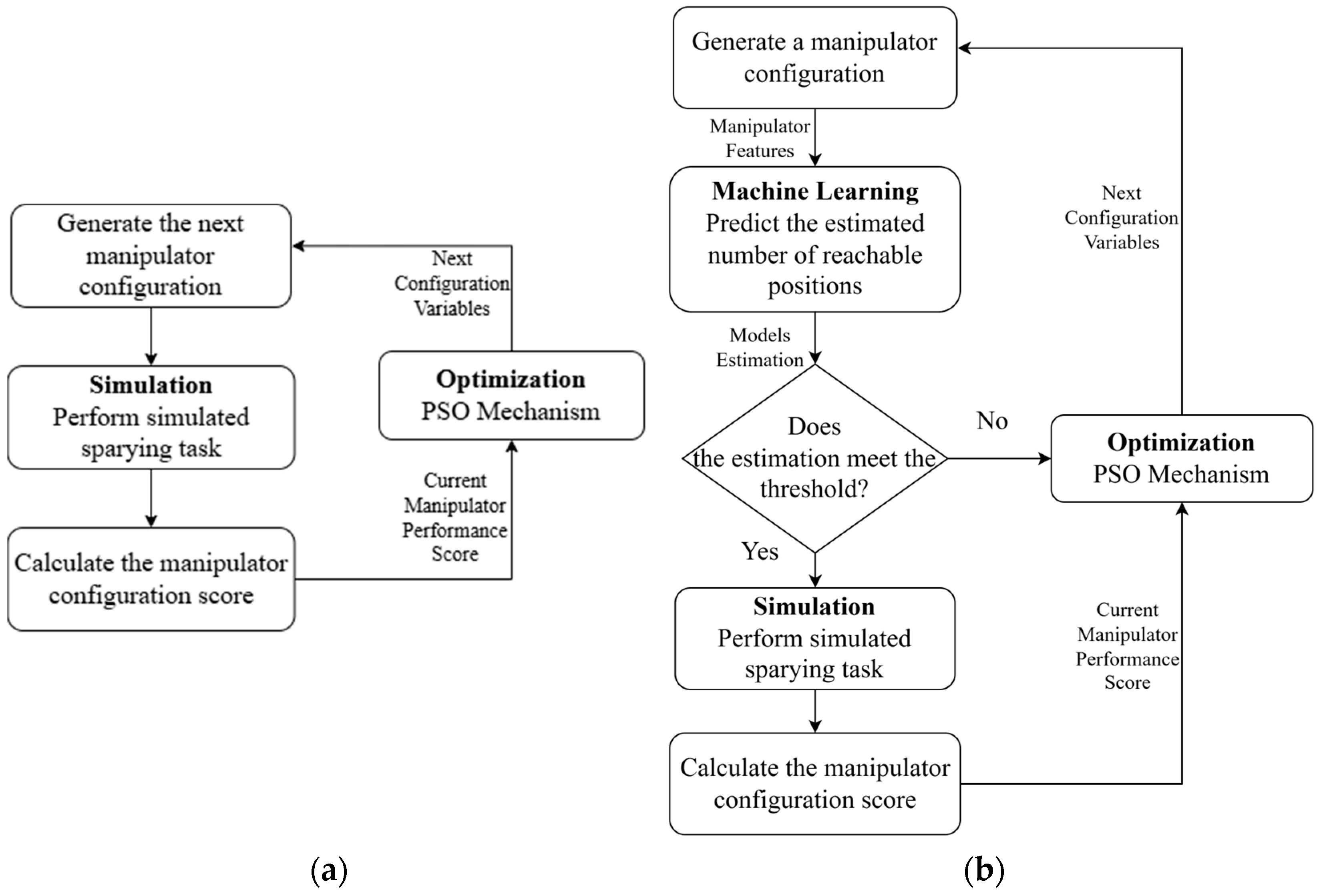
3. Improved Methodology Development

The current methodology to characterize an optimal robot design (Figure 5a) for a specific task involves the use of simulations and optimization algorithms. Simulation serves as a testing tool for evaluating proposed configurations, examining the robot in the task environment by providing the performance scores. In most cases, the solution space is vast, and it is impractical to test every possible solution. Therefore, an optimization algorithm is a tool to strategically select subsequent solutions for examination. This approach enables a search within the solution space, and identifies potential directions for progress, ultimately leading toward an optimal solution, or if applicable, a satisfying solution. The improved methodology (Figure 5b) proposed in this research integrates a ML model to reduce the optimization runtime. The ML model predicts, in turn, the selected manipulator’s ability to comply with the reachability constraint in the simulated environment and task. Configurations that do not comply with the reachability constraint are systematically excluded from the optimization process. This reduces the computational load and runtime, streamlining the optimization workflow and enhancing its overall efficiency.

Flow of the methodologies:

Current methodology:

• A robotic manipulator configuration is generated.
• The manipulator directly performs a simulated task.
• Performance indicators are calculated from the simulation.
• These results feed into a PSO mechanism.
• The PSO mechanism then influences the next generation of manipulator configuration.

The key characteristic of this approach is its direct execution without validation checks, making it simpler but less efficient.

Improved methodology:

The improved methodology introduces a validation layer using XGBoost models before task execution:

• A robotic manipulator configuration is generated.
• Trained XGBoost models are loaded to validate the configuration.
• A decision point checks if the manipulator is expected to reach the threshold.
• Only configurations passing this validation proceed to the simulation.
• Performance indicators are calculated only for valid configurations.
• The PSO mechanism optimizes based on these results.

The two options of the methodology presented were compared and discussed in Section 4.3.

4. Results and Discussions

4.1. PSO Hyperparameter Tuning

The hyperparameters of the PSO algorithm were systematically tuned to optimize performance. The tuning process employed a comprehensive grid search methodology using the dataset collected as described in Section 2.3.1. Each hyperparameter combination was evaluated through 30 independent PSO runs. Performance was assessed using the average reachability score across all runs, with the optimal hyperparameter set determined by identifying the configuration that consistently achieved the highest mean performance. The hyperparameters tuned in this study included the following:

1.

Inertia Weight (ω): The inertia weight is a critical parameter influencing the performance of the PSO algorithm. It determines how much of a particle’s previous velocity is retained in its current iteration, effectively controlling the momentum of particles. A higher inertia weight promotes global exploration by encouraging particles to move into new regions of the search space, while a lower value facilitates local exploitation by focusing on refining existing solutions. It was adjusted by using three different strategies: (i) a constant parameter value of 0.795, (ii) a linear function decreasing in time with the set $\left\{{\omega }_{max}=0.9,{\omega }_{min}=0.4\right\},$ and (iii) a chaotic linear decreasing with the set $\left\{{\omega }_{max}=0.9,{\omega }_{min}=0.4\right\}$.

2.

Population Size: The population size represents the number of individual particles or potential solutions maintained simultaneously in the swarm during the PSO algorithm’s execution. Each particle represents a candidate solution to the optimization problem and moves through the search space based on its own experience and the collective knowledge of the swarm. The population size is determined by the specific problem being addressed; however, it is generally not highly sensitive to variations in problem characteristics [31]. The options considered were population sizes of 20 or 50 particles.

The selected hyperparameters:

• Inertia Weight (ω): Chaotic inertia weight. The fundamental concept of the chaotic inertia weight method involves using a chaotic map to set the inertia weight coefficient. In this method, the Logistic mapping is used to achieve this. The formula for Logistic mapping is as follows:

  $$z=\mu z(1-z)$$

  (23)

  where $3.57\le \mu \le 4$ Logistic mapping occurs as chaotic phenomena.

Therefore, by this method, in each algorithm’s iteration, first a Logistic mapping is performed:

$$z_{k+1}=4z_k\left(1-z_k\right)$$

(24)

Then, the coefficient is calculated as follows:

$${\omega }_{iter}=\left({\omega }_{initial}-{\omega }_{final} \right)\left[{\displaystyle \frac{Ite{r}_{max} -Iter}{Ite{r}_{max}}}\right]+{\omega }_{final}\ast z_{k+1}$$

(25)

2.

Population Size: set to 50.

3.

Cognitive Coefficient (c1) and Social Coefficient (c2): Both coefficients were set to 1.49, reflecting a balanced influence between a particle’s personal best position and the swarm’s best-known position.

4.

Generation Number (Iterations): The number of generations was set to 200 due to computational considerations.

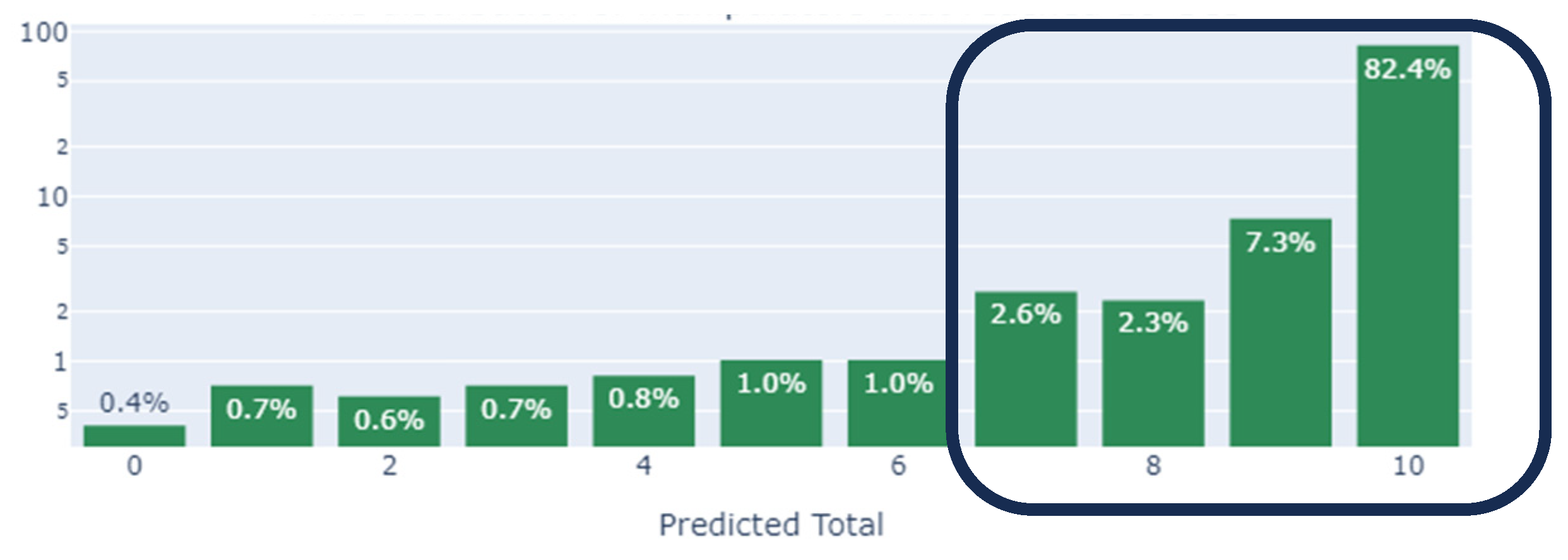
4.2. ML Training Results

In early stages of this study, several ML models, including Random Forest and SVM, were tested for the discussed classification task but demonstrated inferior performance compared to XGBoost in terms of accuracy. Therefore, this study focused on evaluating the effectiveness of the improved methodology consisting of PSO and XGBoost in comparison to the current methodology, rather than benchmarking it against other machine learning approaches. However, future work could explore comparisons with neural networks or other ensemble methods to further assess performance differences.

To address the issue of imbalanced binary classification, the models were adjusted by scaling the gradient specifically for the positive class of each target. Ten individual XGBoost models were trained, each aimed at predicting reachability to a specific position within the simulated vineyard environment. Each of the ten target positions in the simulation represent a grape cluster (GC). These models were evaluated as binary classifiers. The performance of these models was appraised by calculating the PPV and NPV. Misclassifications, including false positives and false negatives, can occur due to the model’s sensitivity to specific patterns or noise in the data. False positives may arise when the model overestimates the relevance of certain features, while false negatives can occur when the model fails to recognize positive instances due to insufficiently distinctive features. The average scores achieved were 0.824 for the PPV and 0.831 for the NPV, as shown in

Table 2. NPV and PPV results.

Position Predicted	NPV	PPV
GC1	0.884	0.862
GC2	0.865	0.856
GC3	0.843	0.82
GC4	0.835	0.827
GC5	0.85	0.833
GC6	0.835	0.822
GC7	0.815	0.804
GC8	0.819	0.803
GC9	0.825	0.815
GC10	0.794	0.795
Average	0.831	0.824

, indicating a high level of accuracy in predicting the correct classification for each position. To account for prediction errors and misclassifications, a threshold value was established to manage the balance between model accuracy and potential runtime reduction.

Figure 6 represents the distributions of the sum of the predictions made by the ten ML models, only for the manipulators with full reachability that successfully reached all ten desired positions in the simulation. The distribution of predictions for these manipulators is analyzed to determine the threshold value. By analyzing the results in Figure 6, a threshold value of seven positions was identified as effective in capturing 94.6% of configurations. This threshold encompasses the main clusters of accurate predictions and reduces the risk of overlooking true optimal configurations. Setting the threshold to seven indicates that, during the optimization process, only manipulators predicted to be capable of reaching at least seven of the required positions are selected for simulation. Manipulators predicted to achieve fewer positions are assigned a score of 0, excluding them from consideration as optimal configurations. This approach substantially enhances the efficiency of the testing process by concentrating on the most promising configurations, thus reducing runtime and increasing the likelihood of identifying optimal solutions.

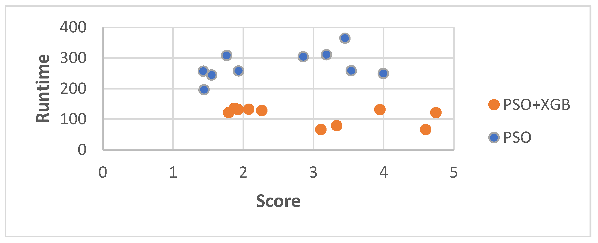
4.3. Methodologies Comparison

The ML models in the improved methodology serve as a decision-making mechanism to put forward a potential configuration for testing in the simulation, thereby reducing the simulation runtime of configurations that were disqualified for simulation. The comparison between the current and improved methodologies was conducted using ten repetitions across ten distinct condition combinations. For each condition combination of seed and initial solution, both the current and improved methodologies were applied, maintaining identical initial conditions. This design ensured that each run (e.g., run number 1, 2, 3…10) shared the same initial state for the PSO algorithm. The experimental results are detailed in

Table 3. Current and improved methodologies comparison results. The red color represents negative values (i.e., the PSO+XGB values are lower than the PSO values) and the blue color represents positive values.

Rep.	Performance Score		Optimal Manipulator [Link Family No., Joint Family No.]		Runtime [Mins]		Runtime Difference (%)	Score Difference (%)
	PSO	PSO + XGB	PSO	PSO + XGB	PSO	PSO + XGB
1	1.43	1.926	[334, 3616]	[328, 3854]	256.98	131.37	−48.88%	34.69%
2	1.763	2.078	[152, 1958]	[118, 1856]	308.18	132.23	−57.09%	17.87%
3	3.449	2.264	[270, 6787]	[280, 2896]	364.67	127.87	−64.94%	−34.36%
4	2.855	4.745	[268, 6794]	[268, 6787]	303.85	121.02	−60.17%	66.20%
5	1.4409	1.791	[435, 2794]	[454, 6087]	196.32	121.10	−38.31%	24.3%
6	3.538	3.106	[270, 289]	[287, 295]	258.37	65.88	−74.50%	−12.21%
7	3.185	3.947	[381, 3152]	[420, 6078]	310.68	131.03	−57.82%	23.92%
8	1.55	4.599	[199, 4461]	[119, 2691]	244.05	65.97	−72.97%	196.71%
9	3.996	3.33	[119, 2383]	[119, 1575]	249.25	78.53	−68.49%	−16.66%
10	1.933	1.876	[281, 289]	[251, 3117]	257.52	135.52	−47.37%	−2.95%
Avarage	2.514	2.97			275.99	111.95	−59.06%	29.75%

. The superiority of the improved methodology is expressed in the following two main performances:

• Runtime: As illustrated in Figure 7, the improved methodology significantly reduced runtime compared to the current methodology. The use of XGBoost reduced the average runtime by 59.06%, demonstrating a substantial increase in computational efficiency. Both methodologies used PSO with 200 iterations.
• Optimization objective score: In the improved methodology, the manipulability index, in six out of the ten runs, achieved higher optimization objective scores, with an average increase of 29.75% in comparison to the current methodology. This indicates that the improved methodology can also potentially achieve higher-quality solutions.

In Table 3, decreases in the performance differences between PSO + XGB (improved methodology) and PSO (current methodology) are denoted in red, while increases are shown in blue.

The results obtained are specific to the experimental setup and conditions under which the comparison was conducted. The 59.06% runtime reduction and the observed improvements in the objective scores were achieved through the use of XGBoost as a part of the optimization process. The comparison was conducted to evaluate the contribution of the XGBoost model rather than to benchmark different optimization techniques. Therefore, while the improvements demonstrated in this study are significant for the given problem, further research comparing the proposed methodology with other optimization methods could provide a more comprehensive understanding of the performance in broader contexts.

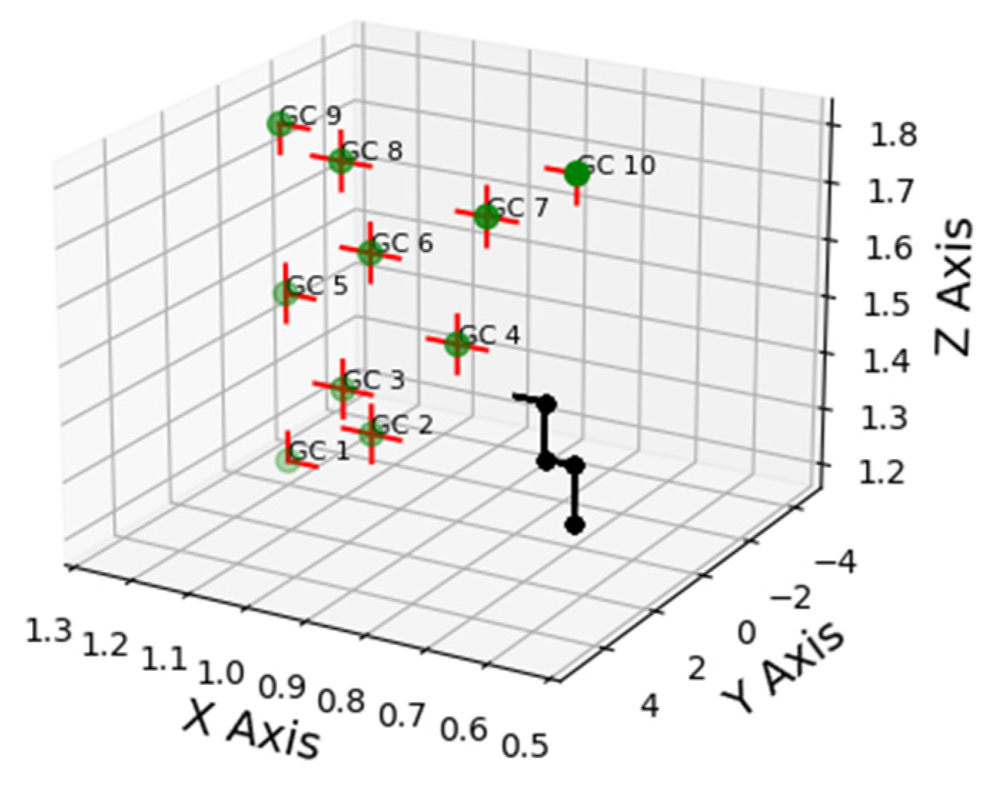
4.4. Optimal Manipulator

To determine the optimal manipulator configuration for the case study presented in this research, a comprehensive analysis was conducted to evaluate the best manipulators determined in the improved methodology. Ten optimal solutions defined in the ten repetitions for each methodology concept were selected, resulting in a total of 20 candidate configurations. The evaluation included reaching 43 positions in total (Figure 8), consisting of the 10 original target positions and an additional 4 offset positions, 5 cm on each side of the original target positions on the X and Z axes. Seven new positions exceeded the workspace boundaries, as illustrated in Figure 8, and were not regarded. Increasing the number of positions ensures a thorough assessment of the manipulators’ effectiveness and robustness, providing a comprehensive view of their performance across a broader range of operational scenarios.

Table 4. Performance of the top manipulators in the extended experiment, filtered first by reachability and then by manipulability score.

	Manipulator Configuration [Link Family No., Joint Family No.]	Reachability	Performance Score	Methodology
1	[420, 6078]	43	3.702	PSO + XGB
2	[381, 3152]	43	3.105	PSO
3	[270, 289]	43	2.691	PSO
4	[268, 6787]	43	2.301	PSO + XGB
5	[287, 295]	43	2.091	PSO + XGB
6	[454, 6087]	43	1.697	PSO + XGB
7	[435, 2794]	43	1.407	PSO
8	[199, 4461]	43	1.403	PSO
9	[281, 289]	43	1.36	PSO
10	[268, 6794]	43	1.3	PSO
11	[251, 3117]	43	1.066	PSO + XGB
12	[328, 3854]	43	0.991	PSO + XGB
13	[280, 2896]	43	0.513	PSO + XGB
14	[334, 3616]	43	0.34	PSO
15	[270, 6787]	9	5.098	PSO
16	[152, 1958]	27	1.765	PSO
17	[118, 1856]	37	1.657	PSO + XGB
18	[119, 1575]	10	1.439	PSO + XGB
19	[119, 2691]	39	0.826	PSO + XGB
20	[119, 2383]	42	0.589	PSO

presents information on the best 20 manipulators. The results are organized by reachability and then by manipulability score for the 43 positions. A total of 70% of the manipulators managed to meet the extended task requirements and reached all positions. The best manipulator achieved a manipulability index score of 3.702 (Figure 9).

The results in Table 4 and Figure 8 also allow us to compare the two methodologies examined. Both methodologies demonstrate good reachability scores, with maximum reachability in 7 out of 10 configurations for each methodology. These results suggest that both algorithms can identify manipulator configurations capable of reaching all target positions.

In terms of the performance index and manipulability score, the current methodology (PSO) achieved an average score of 1.658 across configurations that met all 43 target positions, with a highest score of 3.105. The improved methodology achieved the highest individual score of 3.702 and an average score of 1.765.

5. Conclusions

In this study, an improved methodology to characterize the optimal robot manipulator for a specific task was developed. The methodology involves formulating the selection of manipulator configuration parameters as a discrete optimization problem, employing the PSO algorithm, and using ML models as predictors for excluding suboptimal solutions in the optimization process. The results indicate that the proposed methodologies can yield an optimal manipulator design capable of satisfying operational constraints within agricultural workspaces.

The integration of ML, particularly the incorporation of the XGBoost models into the optimization process, has proven highly advantageous and significantly accelerated the convergence of the optimization algorithm. Moreover, by reducing the computational time, this approach allows the exploration of a broader solution space, ultimately leading to the discovery of improved solutions. The findings of this research underscore the significant benefits of utilizing ML models in manipulator design.

In conclusion, both methodologies successfully identify feasible manipulator configurations achieving the reachability with a high performance index score. The improved methodology significantly reduces runtime, allowing the optimization process to run multiple runs in a shorter timeframe, which can potentially offer greater manipulability score results. This efficiency allows for more iterations, potentially resulting in improved manipulator configurations and validation of results.

While this study is based on simulations, real-world validation is essential to confirm the practical applicability of the proposed methodology. Future research could explore implementing optimized manipulator configurations in a physical robotic system and conducting experimental trials in a vineyard environment. These experiments could assess factors such as motion accuracy, mechanical feasibility, and adaptability to real-world complexities, including uneven terrain and dynamic obstacles, such as moving branches. Additionally, integrating real sensor data into the optimization process could further refine the model’s predictive accuracy and bridge the gap between simulation and practical deployment.

References

1. Alrashdi, A.M.A.; Al-Qurashi, A.D.; Awad, M.A.; Mohamed, S.A.; Al-rashdi, A.A. Quality, antioxidant compounds, antioxidant capacity and enzymes activity of ‘El-Bayadi’ table grapes at harvest as affected by preharvest salicylic acid and gibberellic acid spray. Sci. Hortic. 2017, 220, 243–249. [Google Scholar] [CrossRef]
2. Berenstein, R.; Shahar, O.B.; Shapiro, A.; Edan, Y. Grape clusters and foliage detection algorithms for autonomous selective vineyard sprayer. Intell. Serv. Robot. 2010, 3, 233–243. [Google Scholar] [CrossRef]
3. Danton, A.; Roux, J.C.; Dance, B.; Cariou, C.; Lenain, R. Development of a spraying robot for precision agriculture: An edge following approach. In Proceedings of the CCTA 2020-4th IEEE Conference on Control Technology and Applications, Montreal, QC, Canada, 24–26 August 2020; pp. 267–272. [Google Scholar] [CrossRef]
4. Fountas, S.; Mylonas, N.; Malounas, I.; Rodias, E.; Santos, C.H.; Pekkeriet, E. Agricultural robotics for field operations. Sensors 2020, 20, 2672. [Google Scholar] [CrossRef] [PubMed]
5. García-Vanegas, A.; García-Bonilla, M.J.; Forero, M.G.; Castillo-García, F.J.; Gonzalez-Rodriguez, A. AgroCableBot: Reconfigurable Cable-Driven Parallel Robot for Greenhouse or Urban Farming Automation. Robotics 2023, 12, 165. [Google Scholar] [CrossRef]
6. Wang, D.; Tan, D.; Liu, L. Particle swarm optimization algorithm: An overview. Soft Comput. 2018, 22, 387–408. [Google Scholar] [CrossRef]
7. Bechar, A.; Vigneault, C. Agricultural robots for field operations. Part 2: Operations and systems. Biosyst. Eng. 2017, 153, 110–128. [Google Scholar] [CrossRef]
8. Zhou, L.; Bai, S. A new approach to design of a lightweight anthropomorphic arm for service applications. J. Mech. Robot. 2015, 7, 031001. [Google Scholar] [CrossRef]
9. Xiao, Y.; Fan, Z.; Li, W.; Chen, S.; Zhao, L.; Xie, H. A Manipulator Design Optimization Based on Constrained Multi-objective Evolutionary Algorithms. In Proceedings of the 2016 International Conference on Industrial Informatics-Computing Technology, Intelligent Technology, Industrial Information Integration (ICIICII), Wuhan, China, 3–4 December 2016; pp. 199–205. [Google Scholar] [CrossRef]
10. Meir, I.; Bechar, A.; Sintov, A. Kinematic Optimization of a Robotic Arm for Automation Tasks with Human Demonstration. In Proceedings of the 2024 IEEE International Conference on Robotics and Automation (ICRA), Yokohama, Japan, 13–17 May 2024; pp. 7172–7178. [Google Scholar] [CrossRef]
11. Shirazi, A.R.; Fakhrabadi, M.M.S.; Ghanbari, A. Optimal design of a 6-DOF parallel manipulator using particle swarm optimization. Adv. Robot. 2012, 26, 1419–1441. [Google Scholar] [CrossRef]
12. Farooq, S.S.; Baqai, A.A.; Shah, M.F. Optimal design of tricept parallel manipulator with particle swarm optimization using performance parameters. J. Eng. Res. 2021, 9, 378–395. [Google Scholar] [CrossRef]
13. Ore, J.; Detweiler, C.; Elbaum, S. Towards Code-Aware Robotic Simulation Vision Paper. In Proceedings of the 1st International Workshop on Robotics Software Engineering, Gothenburg, Sweden, 28 May 2018; pp. 40–43. [Google Scholar]
14. Zhibao, S.; Haojie, Z.; Sen, Z. A robotic simulation system combined USARSim and RCS library. In Proceedings of the 2017 2nd Asia-Pacific Conference on Intelligent Robot Systems (ACIRS), Wuhan, China, 16–19 June 2017; pp. 240–243. [Google Scholar] [CrossRef]
15. Wang, H.; Hohimer, C.J.; Bhusal, S.; Karkee, M.; Mo, C.; Miller, J.H. Simulation as A Tool In Designing and Evaluating A Robotic Apple Harvesting System. IFAC-PapersOnLine 2018, 51, 135–140. [Google Scholar] [CrossRef]
16. Takaya, K.; Asai, T.; Kroumov, V.; Smarandache, F. Simulation environment for mobile robots testing using ROS and Gazebo. In Proceedings of the 2016 20th International Conference on System Theory, Control and Computing (ICSTCC), Sinaia, Romania, 13–15 October 2016; pp. 96–101. [Google Scholar] [CrossRef]
17. Huang, Z.; Li, F.; Xu, L. Modeling and simulation of 6 DOF robotic arm based on gazebo. In Proceedings of the 2020 6th International Conference on Control, Automation and Robotics (ICCAR), Singapore, 20–23 April 2020; pp. 319–323. [Google Scholar] [CrossRef]
18. Karoly, A.I.; Galambos, P.; Kuti, J.; Rudas, I.J. Deep Learning in Robotics: Survey on Model Structures and Training Strategies. IEEE Trans. Syst. Man Cybern. Syst. 2021, 51, 266–279. [Google Scholar] [CrossRef]
19. Pierson, H.A.; Gashler, M.S. Deep learning in robotics: A review of recent research. Adv. Robot. 2017, 31, 821–835. [Google Scholar] [CrossRef]
20. Yue, S.; Shi, Y. Manipulator Smooth Control Method Based on LSTM-XGboost and Its Optimization Model Construction. Appl. Sci. 2023, 13, 8994. [Google Scholar] [CrossRef]
21. Lin, X.; Wang, Z.-Q.; Chen, X.-Y. Path Planning with Improved Artificial Potential Field Method Based on Decision Tree. In Proceedings of the 2020 27th Saint Petersburg International Conference on Integrated Navigation Systems (ICINS), Saint Petersburg, Russia, 25–27 May 2020. [Google Scholar] [CrossRef]
22. Yoo, J.-H.; Park, Y.-K.; Han, S.-S. Predictive Maintenance System for Wafer Transport Robot Using K-Means Algorithm and Neural Network Model. Electronics 2022, 11, 1324. [Google Scholar] [CrossRef]
23. Lenz, I.; Lee, H.; Saxena, A. Deep learning for detecting robotic grasps. Int. J. Robot. Res. 2015, 34, 705–724. [Google Scholar] [CrossRef]
24. Wu, J.; Yildirim, I.; Lim, J.J.; Freeman, W.T.; Tenenbaum, J.B. Galileo: Perceiving physical object properties by integrating a physics engine with deep learning. Adv. Neural Inf. Process. Syst. 2015, 28, 127–135. [Google Scholar]
25. McArthur, C. Embed to Control: A Locally Linear Latent Dynamics Model for Control from Raw Images. Cine. J. 2008, 47, 147–152. [Google Scholar] [CrossRef]
26. Oberti, R.; Marchi, M.; Tirelli, P.; Calcante, A.; Iriti, M.; Tona, E.; Hočevar, M.; Baur, J.; Pfaff, J.; Schütz, C.; et al. Selective spraying of grapevines for disease control using a modular agricultural robot. Biosyst. Eng. 2016, 146, 203–215. [Google Scholar] [CrossRef]
27. Wandkar, S.V.; Bhatt, Y.C.; Jain, H.K.; Nalawade, S.M.; Pawar, S.G. Real-Time Variable Rate Spraying in Orchards and Vineyards: A Review. J. Inst. Eng. (India) Ser. A 2018, 99, 385–390. [Google Scholar] [CrossRef]
28. Yoshikawa, T. Manipulability of Robotic Mechanisms. Int. J. Robot. Res. 1985, 4, 439–446. [Google Scholar] [CrossRef]
29. Qian, W.; Xia, Z.; Xiong, J.; Gan, Y.; Guo, Y.; Weng, S.; Deng, H.; Hu, Y.; Zhang, J. Manipulation task simulation using ROS and Gazebo. In Proceedings of the 2014 IEEE International Conference on Robotics and Biomimetics (ROBIO 2014), Bali, Indonesia, 5–10 December 2014; pp. 2594–2598. [Google Scholar] [CrossRef]
30. Eberhart, R.; Kennedy, J. A new optimizer using particle swarm theory. In MHS ’95: Proceedings of the Sixth International Symposium on Micro Machine and Human Science; Nagoya Municipal Industrial Research Institute: Nagoya, Japan, 1995; pp. 39–43. [Google Scholar]
31. Ahmed, A.A.W.; Markendahl, J.; Ghanbari, A. Development of An Autonomous Kiwifruit Picking Robot. In Proceedings of the 2009 4th International Conference on Autonomous Robots and Agents, Wellington, New Zealand, 10–12 February 2009; pp. 1–5. Available online: https://ieeexplore.ieee.org/document/4804023/authors#authors (accessed on 18 April 2025).
32. Shi, Y.H.; Eberhart, R. Modified particle swarm optimizer. In Proceedings of the 1998 IEEE International Conference on Evolutionary Computation Proceedings (ICEC), Anchorage, AK, USA, 4–9 May 1998; pp. 69–73. [Google Scholar] [CrossRef]
33. Yan, K. Student performance prediction using XGBoost method from a macro perspective. In Proceedings of the 2021 2nd International Conference on Computing and Data Science (CDS), Stanford, CA, USA, 28–29 January 2021; pp. 453–459. [Google Scholar] [CrossRef]
Figure 1. The Y-shaped experiment’s vineyard.
Robotics 14 00058 g001
Figure 2. Illustration of a potential manipulator configuration performing the simulated spraying task. (a) Demonstration in the Rviz simulator; (b) demonstration in Gazebo.
Robotics 14 00058 g002
Figure 3. Description of robot’s workspace.
Robotics 14 00058 g003
Figure 4. The grape cluster (the targets) positions in the simulation illustrated in 3D. The green circles represents the cluster’s position; the black line represents the robotic manipulator.
Robotics 14 00058 g004
Figure 5. The framework of the two compared methodologies: (a) current optimization methodology; (b) improved optimization methodology.
Robotics 14 00058 g005
Figure 6. Distributions of cumulative predictions by ML models for manipulators that meet full reachability.
Robotics 14 00058 g006
Figure 7. Comparison of Runtime vs. Score for current methodology (PSO) and the improved methodology (PSO + XGB).
Robotics 14 00058 g007
Figure 8. Final experiment target positions. The green circles represents the cluster’s position; the black line represents the robotic manipulator. The red cross represents the additional positions.
Robotics 14 00058 g008
Figure 9. Illustration of the optimal manipulator selected. (a) The configuration is demonstrated in the Rviz simulator; (b) demonstrated in Gazebo.
Robotics 14 00058 g009