A New Proposal for Intelligent Continuous Controller of Robotic Finger Prostheses Using Deep Deterministic Policy Gradient Algorithm Through Simulated Assessments

Abstract

To improve the adaptability of the hand prosthesis, we propose a new smart control for a physiological finger prosthesis using the advantages of the deep deterministic policy gradient (DDPG) algorithm. A rigid body model was developed to represent the finger as a training environment. The geometric characteristics and physiological physical properties of the finger available in the literature were assumed, but the joint’s stiffness and damping were neglected. The standard DDPG algorithm was modified to train an artificial neural network (ANN) to perform two predetermined trajectories: linear and sinusoidal. The ANN was evaluated through the use of a computational model that simulated the functionality of the finger prosthesis. The model demonstrated the capacity to successfully execute both sinusoidal and linear trajectories, exhibiting a mean error of $3.984\pm 2.899$ mm for the sinusoidal trajectory and $3.220\pm 1.419$ mm for the linear trajectory. Observing the torques, it was found that the ANN used different strategies to control the movement in order to adapt to the different trajectories. Allowing the ANN to use a combination of both trajectories, our model was able to perform trajectories that differed from purely linear and sinusoidal, showing its ability to adapt to the movement of the physiological finger. The results showed that it was possible to develop a controller for multiple trajectories, which is essential to provide more integrated and personalized prostheses.

1. Introduction

Transradial robotic prostheses are essential devices to improve amputees’ activities of daily living (ADL). Despite current advances in the actuators and control systems, these devices lack the ability to adapt movements during the ADL [1]. Myoelectric prostheses are the state of art in upper limb prostheses and aim to translate superficial electromyography (sEMG) signals into the desired user’s movement using artificial intelligence algorithms [1,2,3]. The sEMG measures the electric potentials generated by the muscular motor units, i.e., it is a non-invasive technique to read neuronal commands, which is crucial for an ideal prosthesis control system [2,4,5]. For example, Liao et al. [6] propose a neural network-based recognition algorithm for sEMG signal envelopes in order to develop a low-cost interface for collaborative wearable robots.

The prediction of the desired movement through sEMG occurs using pattern recognition (PR) algorithms, where the sEMG is correlated with a grasp motion, and the movement that is closest to the natural movement is selected [7,8]. This correlation could be structured using classic techniques, e.g., artificial neural networks (ANNs), linear discriminant analysis (LDA) and support vector machines (SVMs) [9,10]. Although the accuracy, which is superior to 90%, as shown in Guo et al. [11] and Vásconez et al. [8], demonstrates their effectiveness, the insufficiency of these strategies lies in the adjustability of the movements, because after selection, the grasp is perform by the device using a state machine, i.e., the motion is always the same and does not adapt to environmental conditions [9]. This inability to adapt limits the user’s capabilities with the devices during their ADL, since the motions are non-patterned and require complex combinations of the joints’ movements [9,12].

In order to adapt to the environment, some authors have studied and investigated new ways of controlling the devices. The high-density sEMG sensors can be used to determine the desired movement by indicating which fingers should be flexed or extended instead of associating them with only a grasping movement [13]. Another way of achieving better integration of the device with the environment is through exclusive control of the contact force on the fingers, thus ensuring that once objects are grasped by the prosthesis, they do not slip. To do this, there are studies in the literature that demonstrate the great effectiveness of these systems using proportional derivative controllers (PIDs) and Fuzzy and predictive modeling with Kalman filters [14,15]. Although they manage to improve the way the device manipulates the objects, these controllers still do not control the movement of the fingers, but rather ensure that the objects are firmly grasped by the prosthesis.

To improve the integration of the user with the prosthesis during the ADL, a new controller system is needed, using the sEMG signal to determine the kinematic state of each joint, to induce the device to perform non-patterned movements [1,9]. Some authors tried to use regression algorithms to discretize the joints’ positions; however, these models depend on several parameters (e.g., joint stiffness, mass, center of mass), which change for each user [16,17]. In order to make the prosthesis more adaptive to the environment and to users, it is essential to develop systems capable of implementing control strategies that are adaptive to both the environment and the user. In the literature, some authors have shown that in the iterations of robots with humans it is necessary to introduce adaptive controls such as torque and impedance [18,19]. In addition, the use of deep reinforcement learning (DRL) techniques has shown great ability to create adaptive robots, such as a robotic eel, that are able to extract optimal movement strategies from the environment in which they are inserted [20]. Thus, DRL techniques have enabled the creation of intelligent controllers that can control complex mechanical systems with a degree of disturbance, a scenario observed in upper limb prostheses during ADLs [20,21].

One of the most used DRL techniques is the deep deterministic policy gradient (DDPG), which has been used to perform the motion planning of multi degree of freedom (DOF) robots [22]. The DDPG method, proposed by Lillicrap [23], is being used to solve diverse challenging tasks in different fields, and is gaining popularity in the scientific literature [24,25,26]. The DDPG is a model-free and off-policy algorithm based on a combination of the actor–critic approach and the Deep Q Network (DQN) method [27], which allows the use of a neural network as an approximator function, the implementation of a replay buffer and the use of a separate target network [28]. This RL technique is designed to learn policies in a continuous action space, in a high-dimensional state and with complex non-linear dynamics, making it a competitive solution compared to planning algorithms with full access to the dynamics and derivatives of the domain [29]. Given these properties, the DDPG is widely used in the robotics field because it has demonstrated its efficiency in learning optimal policies for locomotion tasks and complex motor skills by controlling joint angles and speeds [30]. Other RL algorithms can also be used to control robotic devices, such as Proximal Policy Optimization (PPO) and the Soft Actor–Critic (SAC). PPO is a variant of the traditional gradient methods, so it optimizes the policy functions directly without learning the value function, reducing the variance of the gradients and improving convergence as the number of samples increases. Despite this improvement, it has been shown in the literature that for complex tasks, PPO does not present a significant improvement when compared to the DDPG [31]. The SAC algorithm is stochastic and based on the maximum entropy framework, which tends to improve the stability and exploration of the model [20,32]. Although, in theory, the SAC has better efficiency than the DDPG, it has been shown in the literature that as the complexity of the reward function is increased, the performance of the SAC is surpassed by the DDPG [33]. Thus, among the algorithms observed, the DDPG tends to performs successfully when the problem to be solved is complex and when the reward function is complex, which is observed in the problem of controlling robotic prostheses.

Some studies are being conducted to test and evaluate the viability of the DDPG in different controlling systems. Sun et al. [34] designed a traditional Adaptive Cruise Control algorithm, based on the DDPG, covering driving assistance technology, to improve the safety and traffic efficiency performance of three-axle heavy vehicles. Chen and Han [35] proposed an improvement in power extraction efficiency, stabilization of power generation and load decrease in wind turbines, using the DDPG-based adaptive reward technique in wind farms. Chen et al. [36] used the DDPG algorithm to improve the motion performance of hydraulic robotic arms. Despite the extensive use of the DDPG technique in the literature for solutions in different fields of knowledge, the authors did not find any studies using the DDPG for the adaptive control of upper limb prostheses, since the primary focus in the literature was on developing systems to discretize the desired movements or to control grasping, and not to adapt the prosthetic trajectories.

In this context, the aim of this study is to explore the versatility of the DDPG method to train a controller capable of moving a finger of an upper limb prosthesis in multiple adaptive trajectories proportional to the desired trajectory selection. For this purpose, a learning environment was developed, assuming a finger prosthesis with physiological characteristics, using different trajectories for the relative rotation of the phalanges’ joints: a linear trajectory, a sinusoidal trajectory and a combination of linear and sinusoidal trajectories. To investigate the ANN’s performance, the computational model developed as a training environment was used, evaluating the control capabilities in performing the trajectories with different inputs and finger sizes. Therefore, this study proposes a new method for controlling the motion of upper limb prostheses, seeking the evolution of this device.

2. Materials and Methods

In order to better understand the development of this work, the methodological description will be divided as follows: first, we will present the learning environment, defining the dynamic model of the finger and the reward function; and finally, we will present the algorithm used in the learning phase and the ANN model, showing how the trajectories were inserted into the model.

2.1. Learning Environment

The learning environment consisted of a simplified index finger model, where the objective of the ANN model was to find the ideal continuous torque for each finger joint, in such a way that the fingertip followed a predetermined trajectory. To determine the joint states, a rigid body mechanical model was elaborated, which gave, for each torque defined by the ANN, the states desired. The reward function was developed to compare the fingertip spatial position desired with the position calculated using the applied torque. In this section, we present the mathematical model of the index finger, the physical and geometric parameters of the finger, the desired fingertip trajectories and the reward function applied in the learning environment algorithm.

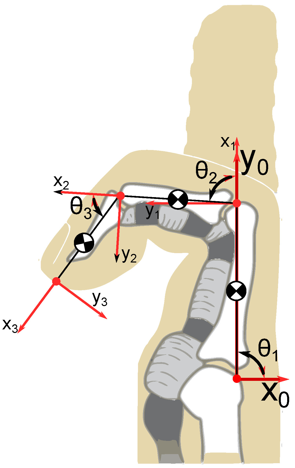
2.1.1. Mathematical Model

For the development of the mathematical description of the model, the method proposed by Spong et al. [37] was used. The index finger was considered to consist of three rigid links (phalanges) connected by three revolutional joints. The joint axes $z_0$, $z_1$, $z_2$ and $z_3$ were normal to the page. The base frame o₀x₀y₀z₀ was defined with the origin at the intersection of the z₀ axis and the page, and the x₀ axis was chosen in the horizontal direction. Once the base frame was established, the o₁x₁y₁z₁, o₂x₂y₂z₂ and o₃x₃y₃z₃ frames were defined, considering the Denavit–Hartenberg convention (Figure 1).

The Euler–Lagrange method was adopted for the development of the motion equations for the three phalanges. Assuming ${\theta }_i$ to be the phalanges’ angles with respect to the $x_{i-1}$-axis, $m_i$ to be the mass of link i, $l_i$ to be the length of link i, $l_{ci}$ to be the distance from the previous joint to the center of mass of link i and $I_i$ to be the moment of inertia of link i about an axis coming out of the page, passing through the center of mass of link i, we have the following equation:

$$\sum _{j=1}^n{d}_{kj}\left(\theta \right)\ddot{{\theta }_j}+\sum _{i=1}^n\sum _{j=1}^n{c}_{ijk}\left(\theta \right)\dot{{\theta }_i}\dot{{\theta }_j}+g_k\left(\theta \right)={\tau }_k,k=1,2,3$$

(1)

where $d_{kj}$ represents the inertia matrix (D($\theta$)) elements, $c_{ijk}$ the Christoffel symbols, $g_k$ the term associated with total gravitational potential energy (P($\theta$)) and ${\tau }_k$ the external torques applied to the joints. The terms, $d_{kj}$, $c_{ijk}$ and $g_k$, of Equation (1), were obtained as follows:

$$D\left(\theta \right)=\sum _{i=1}^n{m}_i{J}_{v_i}{\left(\theta \right)}^T{J}_{v_i}\left(\theta \right)+\left[\begin{array}{ccc}{I}_1+I_2+I_3& I_2+I_3& I_3\\ I_2+I_3& I_2+I_3& I_3\\ I_3& I_3& I_3\end{array}\right]$$

(2)

$$c_{ijk}={\displaystyle \frac{1}{2}}\left({\displaystyle \frac{\partial d_{kj}}{\partial {\theta }_i}}+{\displaystyle \frac{\partial d_{ki}}{\partial {\theta }_j}}-{\displaystyle \frac{\partial d_{ij}}{\partial {\theta }_k}}\right)$$

(3)

$$g_k={\displaystyle \frac{\partial P}{\partial {\theta }_k}}$$

(4)

where $J_{v_i}$ is the linear velocity geometric Jacobian with respect to the center of mass of each link. The explicit Runge–Kutta method of order 5(4) was used to solve the mathematical model, using a time step of 10⁻⁵ s. The angles ${\theta }_1={\displaystyle \frac{\pi }{2}}$ rad, ${\theta }_2=0$ rad and ${\theta }_3=0$ rad were considered for the resting position of the finger (fully extended). The motion range of each joint was $\pi /2$ rad from the resting position, and the ANN model was constrained to be unable to lead any joints to positions beyond this defined range.

2.1.2. Index Finger Parameters

The index finger phalanges were approximated by rigid links with a constant and uniform density equal to 1160 kg·m⁻³ [38], and with geometric characteristics represented by the mean anthropometric measurements of the adult male Spanish population reported in the paper by Vergara et al. [39].

Table 1. Properties of index finger phalanges.

Properties	Proximal Phalanx (i = 1)	Medial Phalanx (i = 2)	Distal Phalanx (i = 3)
$l_i$ (m)	45.30 × 10−3	25.60 × 10−3	24.50 × 10−3
$l_{ci}$ (m)	28.70 × 10−3	17.80 × 10−3	13.40 × 10−3
$m_i$ (kg)	17.10 × 10−3	6.40 × 10−3	3.60 × 10−3
$I_i$ (kg·m2)	3.33 × 10−6	4.36 × 10−7	1.44 × 10−7

indicates the values for the properties used.

2.1.3. Trajectory Equations

Two different expected trajectories were considered for the finger of the upper limb prosthesis to follow during the motion: the linear trajectory and the sinusoidal trajectory. The equations for the two trajectories were developed considering a total range of motion of $\pi /2$ rad in a total time of 1 s for each of the three phalanges. To simulate an sEMG time interaction with the model, the joint states were calculated in a time range of 40 ms [40].

For the linear trajectory, the relative angular rotation equations are shown in Equations (5) and (6), and the relative angular velocities equation is shown in Equation (7).

$${\theta }_1={\displaystyle \frac{\pi }{2}}(t+1)$$

(5)

$${\theta }_2={\theta }_3={\displaystyle \frac{\pi }{2}}t$$

(6)

$${\dot{\theta }}_1={\dot{\theta }}_2={\dot{\theta }}_3={\displaystyle \frac{\pi }{2}}$$

(7)

where t is time. In another way, for the sinusoidal trajectory, the relative angular rotation equations are shown in Equations (8) and (9), and the relative angular velocities equation is shown in Equation (10).

$${\theta }_1={\displaystyle \frac{\pi }{2sin\left({\displaystyle \frac{5\pi }{2}}\right)}}sin\left({\displaystyle \frac{\pi }{2}}t\right)+{\displaystyle \frac{\pi }{2}}$$

(8)

$${\theta }_2={\theta }_3={\displaystyle \frac{\pi }{2sin\left({\displaystyle \frac{5\pi }{2}}\right)}}sin\left({\displaystyle \frac{\pi }{2}}t\right)$$

(9)

$${\dot{\theta }}_1={\dot{\theta }}_2={\dot{\theta }}_3={\displaystyle \frac{{\pi }^2}{4sin\left({\displaystyle \frac{5\pi }{2}}\right)}}cos\left({\displaystyle \frac{\pi }{2}}t\right)$$

(10)

At the end of the learning procedure, the responses obtained by the neural network and the expected responses, given by the previous equations, were compared, as well as the strategies adopted by the ANN to perform the control.

2.1.4. Reward Function and Learning Environment Algorithm

The learning environment has two reward functions: one for situations where the torque determined by the ANN causes a joint angle beyond the allowed range (penalty function), and another reward function that encompasses all the positions allowed for performing the finger motion (reward function). In order to capture the error, an exponential function was used as the basis for both reward functions. The penalty funtion was used when the angle of joint 1 was smaller than $\pi /2$ rad or greater than $\pi$ rad, or if joint 2 or 3 was smaller than 0 rad or greater than $\pi /2$ rad, as shown by Equation (11):

$$R=10exp\left[\left({\displaystyle \frac{ln0.001}{0.5}}\right)\sqrt{{E_1}^2+{E_2}^2+{E_3}^2}\right]-20$$

(11)

where $E_i$ is the amount by which the angle has exceeded the maximum or minimum joint position defined by Equations (12) and (13):

$$E_1=\left\{\begin{array}{cc}{\displaystyle \frac{\pi }{2}}-{\theta }_1,\hfill & {\theta }_1<{\displaystyle \frac{\pi }{2}}\hfill \\ {\theta }_1-\pi ,\hfill & {\theta }_1>\pi \hfill \end{array}\right.$$

(12)

$$E_2=E_3=\left\{\begin{array}{cc}-{\theta }_i,\hfill & {\theta }_i<0\hfill \\ {\theta }_i-{\displaystyle \frac{\pi }{2}},\hfill & {\theta }_i>{\displaystyle \frac{\pi }{2}}\hfill \end{array}\right.i=2,3$$

(13)

The penalty reward function gives penalties between −10 and −20, and was capable of determining better differences between errors in the range between 0 and 0.5 rad. For errors greater than 0.5 rad, the penalty given for the model was approximately the same. In addition, when the angle of any joint was out of the range, the training episode was interrupted.

When the angle of the joints was in the range, the reward function was defined by Equation (14).

$$R=5exp\left[\left({\displaystyle \frac{ln0.001}{0.2}}\right)\sqrt{{E_x}^2+{E_y}^2}\right]-5$$

(14)

where $E_x$ and $E_y$ were the errors between the desired fingertip position and the results obtained by the ANN action, on the x and y coordinates, respectively. The reward function must always give rewards greater than the penalty function, to ensure that the model distinguishes the out-of-range positions in the joints and the allowable positions. In that way, the range of the reward function varied between 0 and −5, and the map absolute errors varied between 0 and 0.2 m, resulting in approximately the same reward for an error greater than 0.2 m. The learning environment and the reward function were implemented with a Gym library, developed for Python programming language [41].

2.2. ANN Model and Learning Algorithm

The ANN model proposed in this work has two distinct inputs. The first consists of two input neurons, where one of the neurons is activated when the finger needs to make a sinusoidal trajectory (input ${\left(1,0\right)}^{⊺}$), while the other is activated to perform the linear trajectory (input ${\left(0,1\right)}^{⊺}$). Following the first input, 3 hidden layers were defined with 8, 4 and 4 neurons, respectively, and the last hidden layer of the first input was concatenated with the neurons of the second input. The second input referred to the current states of the finger, i.e., it had six input neurons. Following the neurons of the second input that were concatenated with the last layer of hidden neurons of the first input, 4 hidden layers were used, with 256, 256, 128 and 32 neurons, respectively. The leaky RELU activation function was used for all the neurons in the hidden layer, with a coefficient of 0.3 for the negative slope. The output layer had three neurons with the hyperbolic tangent activation function and represented the torque commands for the joints. The initialization parameters were randomly set between −0.05 and 0.05 to start the training. The output neurons were scaled by a factor of 0.1 to limit the range of torque applied to the joints.

We used the DDPG training algorithm to determinate the ANN parameter sets. To do this, it was necessary to develop a critic model, represented by another ANN. Three inputs were defined for the critic model: the first input was used for trajectory selection; the second input for the current kinematic states; and the third input for the actions of the ANN actor. The first input was connected to 3 hidden layers with 8, 4 and 4 neurons, respectively, with the last hidden layer concatenated to the second input. Futhermore, the second input was connected to two hidden layers with 64 neurons. The third input was also connected to two hidden layers with 64 neurons; however, it was also concatenated with the last hidden layer of the combination of the first and second inputs. Finally, the combination of all the inputs was connected to three hidden layers with 256 neurons that were connected to a linear output neuron. As in the actor model, all the hidden neurons used the leaky RELU activation function, with a coefficient of 0.3 for the negative slope.

For each training interaction, the ANN tried to perform the sinusoidal trajectory, followed by the linear trajectory. The ANN time step was 1 ms, i.e., the actor had a thousand steps to complete the task and 40 attempts to lead the finger to the next desired position, as previously described. This was determined to emulate an sEMG classifier that determines the desired motion every 40 ms. To ensure the exploration, the Ornstein–Uhlenbeck process was used to generate the noise on the actions, as indicated by the TensorFlow [42] and Keras [43] libraries manual for Python. To periodically check the real performance of the actor ANN every fifty epochs, or if the reward threshold was outperformed, the actor tried to perform the task without the noise, and the training stopped when the reward threshold was overcome. The learning algorithm is presented in Algorithm 1.

All of the training process was performed using the TensorFlow library for Python, and the following parameters were used: an actor learning rate of ${10}^{-4}$; a critic learning rate of ${10}^{-3}$; a buffer size of ${10}^5$; a batch size of 32; the update of the targets networks using a factor $\left(\tau \right)$ of ${10}^{-5}$; a discount factor $\left(\gamma \right)$ of 0.99; and a reward threshold of −650. As shown by Li et al. [22], the efficiency of the training was reduced when only the task failure data were used in training. To maintain the efficiency of the training, we limited the failure samples on buffer and batch to 20% of the total size, i.e., $2\times {10}^4$ and 6, respectively.

Algorithm 1 Modified DDPG Learning Algorithm

Randomly initialize the actor network $\mu \left(i,s|{\theta }^{\mu }\right)$ with the weights ${\theta }^{\mu }$ varying between −0.05 and 0.05 Randomly initialize the critic network $Q\left(i,s,a|{\theta }^Q\right)$ with the weights ${\theta }^Q$ Initialize the target networks ${\mu }^{\prime }\left(i,s|{\theta }^{{\mu }^{\prime }}\right)$ and $Q^{\prime }\left(i,s,a|{\theta }^{Q^{\prime }}\right)$ Initialize the replay buffer Initialize episodes counter $\left(E\leftarrow 0\right)$ while (sinusoidal $\left(R_s\right)$ and linear $\left(R_l\right)$ trajectory reward ≤ −650) and (sinusoidal $S_s$ and linear $S_l$ < 1000) do    Initialize the environment, the agent sinusoidal reward $\left(r_s\leftarrow 0\right)$ and sinusoidal train steps $\left(s_s\leftarrow 0\right)$    Determine the trajectory input $i\leftarrow {\left(1,0\right)}^{⊺}$    for t = 0, 1000 do      Select an action with a noise based on the actual polices $\left(a_t\leftarrow \mu \left(i,s_t|{\theta }^{\mu }\right)+\mathcal{N}\right)$      Execute the action $\left(a_t\right)$ and receive the next states $\left(s_{t+1}\right)$, the step reward $\left(r_t\right)$ and fail or not fail state $\left({\mathcal{F}}_t\right)$      Store the data on buffer $\left(i,s_t,a_t,r_t,s_{t+1},{\mathcal{F}}_t\right)$      Randomly sample a minibatch with 6 fail samples and 26 not fail samples      Get $y_i\leftarrow r_i+\gamma Q^{\prime }\left(i_i,s_{i+1},{\mu }^{\prime }\left(i_i,s_{i+1}|{\theta }^{{\mu }^{\prime }}\right)|{\theta }^{Q^{\prime }}\right)$      Update the critic minimizing the loss: $L_c={\displaystyle \frac{1}{32}}{\sum }_i{\left(y_i-Q\left(i_i,s_i,a_i\right)\right)}^2$      Update the actor minimizing the loss: $L_a=-{\displaystyle \frac{1}{32}}{\sum }_i\left(Q\left(i_i,s_i,\mu \left(i_i,s_i|{\theta }^{\mu }\right)|{\theta }^Q\right)\right)$      Update the targets network: ${\theta }^{Q^{\prime }}\leftarrow \tau {\theta }^Q+(1-\tau ){\theta }^{Q^{\prime }}$ and ${\theta }^{{\mu }^{\prime }}\leftarrow \tau {\theta }^{\mu }+(1-\tau ){\theta }^{{\mu }^{\prime }}$      if any joint is out of range then         break      end if      Set: $r_s\leftarrow r_s+r_t$ and $s_s\leftarrow t$    end for    Initialize the environment, the agent linear reward $\left(r_l\leftarrow 0\right)$ and linear train steps $\left(s_t\leftarrow 0\right)$    Determine the trajectory input $i\leftarrow {\left(0,1\right)}^{⊺}$    for t = 0, 1000 do      Select a action with a noise based on the actual polices $\left(a_t\leftarrow \mu \left(i,s_t|{\theta }^{\mu }\right)+\mathcal{N}\right)$      Execute the action $\left(a_t\right)$ and receive the next states $\left(s_{t+1}\right)$, the step reward $\left(r_t\right)$ and fail not fail state $\left({\mathcal{F}}_t\right)$      Store the data on buffer $\left(i,s_t,a_t,r_t,s_{t+1},{\mathcal{F}}_t\right)$      Randomly sample a minibatch whith 6 fail samples and 26 not fail samples      Get $y_i\leftarrow r_i+\gamma Q^{\prime }\left(i_i,s_{i+1},{\mu }^{\prime }\left(i_i,s_{i+1}|{\theta }^{{\mu }^{\prime }}\right)|{\theta }^{Q^{\prime }}\right)$      Update the critic minimizing the loss: $L_c={\displaystyle \frac{1}{32}}{\sum }_i{\left(y_i-Q\left(i_i,s_i,a_i\right)\right)}^2$      Update the actor minimizing the loss: $L_a=-{\displaystyle \frac{1}{32}}{\sum }_i\left(Q\left(i_i,s_i,\mu \left(i_i,s_i|{\theta }^{\mu }\right)|{\theta }^Q\right)\right)$      Update the target network: ${\theta }^{Q^{\prime }}\leftarrow \tau {\theta }^Q+(1-\tau ){\theta }^{Q^{\prime }}$ and ${\theta }^{{\mu }^{\prime }}\leftarrow \tau {\theta }^{\mu }+(1-\tau ){\theta }^{{\mu }^{\prime }}$      if any joint is out of range then         break      end if      Set: $r_l\leftarrow r_l+r_t$ and $s_t\leftarrow t$    end for    Set $E\leftarrow E+1$    if E is multiple of 50 or ($r_s>-650$ and $s_s$ = 1000) or ($r_l>-650$ and $s_l$ = 1000) then      Get the agent reward for sinusoidal input without noise: $R_s\leftarrow {\sum }_i{r}_i\left(\mu \left({\left(1,0\right)}^{⊺},s_i|{\theta }^{\mu }\right)\right)$      Compute the complete steps with sinusoidal input $\left(S_s\leftarrow {\sum }_i{s}_{s_i}\right)$      Get the agent reward for linear input without noise: $R_l\leftarrow {\sum }_i{r}_i\left(\mu \left({\left(0,1\right)}^{⊺},s_i|{\theta }^{\mu }\right)\right)$      Compute the complete steps with linear input $\left(S_l\leftarrow {\sum }_i{s}_{l_i}\right)$    end if end while

3. Results

3.1. Model Responses for Sinusoidal and Linear Trajectory Inputs

By changing the expected trajectories, it was possible to notice the ANN model’s ability to approximate these two trajectories, as shown in Figure 2. For the sinusoidal trajectory (Figure 2a), the accuracy was worse than that observed on the linear trajectory (Figure 2b); a mean error magnitude of $3.984\pm 2.899$ mm was presented for the sinusoidal compared to $3.220\pm 1.419$ mm for the linear trajectory. In addition, the model was able to smooth the trajectory of the fingertip.

As shown in Figure 2, a similar behavior occurred in both situations: the model trajectory diverged from the expected trajectories according to the increases in the X axis distance, with maximum differences occurring at the point x = −80.25 mm for the sinusoidal trajectory (Figure 2a) and the point x = −78.24 mm for the linear trajectory (Figure 2b). In the sinusoidal condition, a larger discrepancy was observed when it was compared to the linear trajectory at these points; a mean error magnitude of $5.956\pm 3.012$ mm was presented before the trajectory correction and $3.140\pm 2.396$ mm after the correction. For the linear trajectory, the mean error magnitude was $3.396\pm 1.659$ mm before the correction and $3.090\pm 1.195$ mm after the correction.

When analyzing the final stages of the fingertip motion, the ANN model stopped before the desired point (−20.8 mm, −25.6 mm). The ANN model stopped at the point (−25.249 mm, −27.611 mm) for the sinusoidal trajectory, which represents an error magnitude of $4.883$ mm, and it stopped at the point (−25.503 mm, −26.405 mm) for the linear trajectory, representing an error magnitude of $4.772$ mm. Finally, analyzing the error, we observed that for the sinusoidal trajectory, the maximum error magnitude was $16.241$ mm and the minimum was $0.081$ mm, while in the linear trajectory, the maximum error magnitude was $10.563$ mm and the minimum was 0.225 mm.

To better understand the difference observed in Figure 2, Figure 3 shows the torque determined by the ANN model in each joint for both trajectories. It can be seen that the larger torque occurred on joint 1 for the two situations in the first step (Figure 3a,b), with 97.512 N.mm for sinusoidal trajectory and 80.898 N.mm for linear trajectory. Throughout the trajectory, only the low values of torques were applied in order to stabilize the motion. The higher difference occurred when the fingertip reached the maximum distance on the X axis, which was 250 ms for the sinusoidal trajectory and 425 ms for the linear trajectory. At these time points, the control strategy changed drastically. While in the sinusoidal case, a small oscillation on the torque (Figure 3a,c,e) was observed, followed by a zero torque, in the linear situation, more evident oscillations in the torques were observed (Figure 3b,d,f), until the completion of the motion.

Figure 4 shows the state variables of sinusoidal trajectory, relative rotation and relative angular velocity, for all joints. It is possible to see that the shape of the the relative rotation with respect to time was close to the expected curve. Figure 4a,e show that the rotation of joints 1 and 3 ceased before the desired position and became constant after 800 ms. On the other hand, it was observed that the relative rotation of joint 2 nearly achieved the final position (Figure 4c); however, it was achieved prematurely (also at 800 ms). This demonstrates why the fingertip position did not reach the final position of the trajectory, mainly due to the inability of joints 1 and 3 in to achieve the expected position.

The relative angular velocity of joint 1 (Figure 4b), during the sinusoidal trajectory, increased abruptly in the first step, reaching a peak of 7.659 rad/s. This occurred because, in the first step, the finger needed to overcome the inertial forces, and joint 1 was at the greatest distance from the fingertip. After the peak, the velocity reduced and followed the expected curve until it ceased at time 850 ms. Considering joints 2 and 3 (Figure 4d and Figure 4f, respectively), the peak of velocity occurred around 275 ms, i.e., before the correction in the trajectory presented in Figure 2a. This indicates that joints 2 and 3, in the sinusoidal case, were responsible for making the correction. The pattern was close to the expected curve, and the velocity reached zero at around 850 ms, as in joint 1.

The state quantities during the linear trajectory can be observed in Figure 5. The relative rotation closest to the expected linear curve was obtained by joint 1 (Figure 5a), since the final position was lower than expected. The relative rotation of joint 2 (Figure 5c) was also close to linear at the beginning of the motion, and the final position was closer to the desired position than that observed for joint 1. In the relative rotation of joint 3 (Figure 5e), the linearity was impacted by the drastic change observed at 425 ms, which coincides with the point of trajectory correction illustrated in Figure 2b. This behavior could indicate that the correction occurred due to the change in rotation in joint 3.

Regarding the relative angular velocities for the linear trajectory (Figure 5b,d,f), the initial behavior in joint 1 was similar to that observed for the sinusoidal trajectory, with a peak in the first step. However, this was with a smaller magnitude, with a value of 5.069 rad/s. Unlike in the sinusoidal situation, in the linear case, the major relative angular velocity occurred in joint 3, with 8.939 rad/s. The difference in the torque behavior of the joints (Figure 3) was also obtained in the joint velocities, where the linear trajectory also showed an oscillatory behavior around the expected constant velocity. It should be noted that the oscillations occurred when the correction of the trajectory was performed (Figure 2b).

3.2. Model Adaptability Assessment

To evaluate the response of our ANN model acting with a combination of trajectories, we tested mixtures of linear and sinusoidal inputs proportionally to the input neurons. Three proportions were considered for the sinusoidal and linear input neurons, respectively: 0.25 and 0.75 (M2575), 0.5 and 0.5 (M5050) and 0.75 and 0.25 (M7525). The trajectories obtained for each mixture are shown in Figure 6. As expected, the trajectory obtained by the M2575 combination (Figure 6a) was closer to the trajectory observed in the exclusively linear situation (Figure 2b), except for the smoother correction. For the M5050 and M7525 combinations (Figure 6b and Figure 6c, respectively), it can be seen that the trajectories obtained are close to the purely sinusoidal case (Figure 2a). This tendency was expected for the M7525 trajectory, since this combination has a higher proportion of sinusoidal input neurons. For the M5050 combination, we expected that the trajectory was completely different from the linear and sinusoidal situations. All the mixtures showed trajectory correction at the maximum distance from the X axis to the inertial frame, as observed in the purely linear and sinusoidal trajectories.

Table 2. Mean magnitude error in millimeters between mixed trajectories and linear or sinusoidal trajectory.

Model	Trajectories
	M2575	M5050	M7525	Linear	Sinusoidal
M2575	$4.952\pm 2.467$	—	—	$4.428\pm 2.146$	$22.53\pm 10.91$
M5050	—	$5.976\pm 2.973$	—	$17.92\pm 9.607$	$8.178\pm 4.096$
M7525	—	—	$5.001\pm 3.100$	$22.40\pm 12.43$	$4.330\pm 2.429$

shows the mean magnitude errors of the mixture trajectories obtained by the ANN model in relation to the expected trajectories, as well as in relation to the exclusively linear and sinusoidal expected trajectories. The mean magnitude error for M2575 was larger for the sinusoidal case, corroborating the remarks in Figure 6a. In addition, the smaller error was obtained when it was compared to the linear expected trajectory; however, the error was greater than that observed for the purely linear input ($3.220\pm 1.419$ mm). For the M5050 combination, while the smallest error observed was in relation to the desired mixed trajectory, the largest error was obtained in comparison with the purely linear situation. This tendency was observed because this combination was closer to the purely sinusoidal trajectory (Figure 6b). Finally, the M7525 combination showed the lowest error when compared to the exclusively sinusoidal trajectory. Comparing the trajectories of the mixtures obtained by the ANN model and the expected trajectories, an increase in the error was observed when the proportion of the sinusoidal contribution was increased.

Analyzing the torque over time for each joint (Figure 7), the proximity of the torque curves of the combination M5050 and M7525 can be observed, with the torque determined by the model for the sinusoidal input (Figure 3a,c,e). The correction was noticed in the peak between 250 and 350 ms, as observed for the sinusoidal trajectory, with a smaller magnitude for the M5050 trajectory. These observations may demonstrate a reason for the proximity of the trajectory behavior of both inputs to the sinusoidal input. For the M2575 case, it was possible to observe that the oscillation on torque occurred at 400 ms, as was also observed in the torque behavior of the linear input (Figure 3b,d,f). These results may explain the similarity of the M2575 combination to the linear trajectory.

Regarding the state over time, we could observe in the relative angular velocity (Figure 8b,d,f) the same pattern observed in the states for the linear and sinusoidal inputs. For the M2575 input, the velocity after 400 ms oscillated, which enforced the proximity of this input to the linear input (Figure 5). In another way, the M5050 and M7525 inputs presented behavior close to that of the sinusoidal input (Figure 4). As observed in the relative angular position (Figure 8a,c,e), the curves represent, as expected, the behavior closest to the linear input for the M2575 input, and close to the sinusoidal input for the M5050 and M7525 inputs. Moreover, the final position was always the same for all the combinations, with approximately 3.000 rad for joint 1, 1.540 rad for joint 2 and 1.380 rad for joint 3.

Finally, we evaluated the X and Y fingertip positions over time (Figure 9) to better see the proximity of the inputs to the desired output. In both positions, the model’s capability to differentiate the trajectories was clear. For the linear and the M2575 inputs, a proximity to the linear expected positions was observed. In another way, the sinusoidal, M5050 and M7525 inputs were close to the sinusoidal expected positions. When analyzing the component X of the position (Figure 9a), we observed the correction trajectories that occurred in the maximum absolute X position, approximately 250 ms for the sinusoidal and 425 ms for the linear trajectory. Additionally, the final position was observed to be quite similar for all inputs, between 32.5 mm and 35 mm, indicating that the ANN’s strategy after 800 ms was to suspend the stimulation and maintain the position, as illustrated by the torques (Figure 3 and Figure 7). For the Y component of the position (Figure 9b), the values acquired by the ANN were close to those desired, and the correction was less noticeable.

3.3. Model Generality Assessment

In order to assess the generality of the ANN model proposed in this work, three different finger geometric configurations were tested. To modify the geometric configurations, volumetric scales of 90%, 110% and 125% were applied to the original geometry indicated in the Materials and Methods Section (Section 2.1.2). The values of 90% and 110% were selected to capture the observed variability in physiological dimensions, as reported in Vergara et al. [39]. The value of 125% was chosen to extrapolate the physiological variation, thereby simulating a scenario where the finger is heavier and has greater inertia. Figure 10a and Figure 10b show the torque applied to joint 1, i.e., the model’s control strategy, for the 90% scaled geometry during the sinusoidal and linear trajectories, respectively. The mean absolute error observed in that scale was 3.495 ± 2.612 mm on the sinusoidal trajectory and 2.760 ± 1.208 mm on the linear trajectory. Figure 10c and Figure 10d show the control response for finger joint 1 with the volumetric scale of 110% of the original finger size during the sinusoidal and linear trajectories, respectively. The mean absolute error observed in that scale was 4.069 ± 2.963 mm on the sinusoidal trajectory and 3.417 ± 1.752 mm on the linear trajectory. Figure 10e and Figure 10f show the control response for joint 1 in the finger scaled by 125% of the original size during the sinusoidal and linear trajectories, respectively. The mean absolute error observed in that scale was 4.635 ± 3.401 mm on the sinusoidal trajectory and 3.915 ± 2.028 mm on the linear trajectory. The responses of other joints, their states and the responses for the mixed inputs are presented on the Supplementary Materials. Furthermore, it can be noticed that for the smallest scale, 90%, the torque applied to the joints showed a more oscillatory behavior compared to the original geometry, developing oscillation even for the sinusoidal trajectory. For higher scale values, 110% and 125%, the oscillations in the temporal distribution of the torque showed a more damped nature, acquiring a smoother configuration for the 125% scale.

The ANN model, when controlling fingers with different sizes, showed that it was able to identify the modification performed and adapt the control strategy for each environment, altering the torque distribution at the joints throughout the finger’s movement. Moreover, the model maintained different control strategies for each trajectory considered, as observed for the original geometry (Figure 3 and Figure 7). Figure 10 shows that a lighter finger, in the case of 90% scale, resulted in a more oscillatory feature in the torques obtained by the ANN model, i.e., a lower system inertia caused a greater difficulty for the ANN model to control the finger’s motion. This happens because, for a finger with lower inertia, the application of a low torque value could be enough to affect the state of movement of the finger. Consequently, it was necessary for the ANN to apply torques in different directions to ensure that the finger performed the movement in a stable way and without abrupt movements. This demonstrates the model’s ability to detect changes in the geometry and inertial components of each phalanx, indicating the generality of the model developed.

4. Discussion

Observing our results, we could see that the ANN model developed was capable of differentiating the trajectories and creating distinct control strategies according to the trajectory selection inputs, which was the main objective of this study. However, the most promising results were found for the mixed inputs situation. Examining the perspective of controlling upper limb prostheses using sEMG, the pattern recognition technique, which is currently employed, also presents the capacity to select different trajectories inserted into the model. However, the prosthesis tasks are limited by the patterned grips, as presented in work by on Sadikoglu et al. [7] and Vásconez et al. [8]. As demonstrated by the results of the combination of trajectories, we trained the ANN model with only two trajectories and used combinations of different proportions (linear and sinusoidal) to control the motion of the finger. Evaluating the possibility of using sEMG data in conjunction with the ANN model, it would be possible to use kinematic quantities to associate the finger motion with the sEMG features, establishing an indirect relationship between the acquired signal and the prosthesis dynamics. In this way, the ANN model would be capable of providing the user with the possibility of using a different input signal to perform new movements with the prosthesis, as observed with the combination of trajectories. These characteristics demonstrate that the controller developed in this study exhibited a distinct control strategy depending on the previously desired trajectory, suggesting its potential for widespread use in controlling the movement of prostheses. Contrary to existing studies, which have focused on standardized movement control and execution without considering user-specific or activity-specific needs, this controller was designed to adapt to non-standardized movement and activity types [7,8,13]. This adjustment of the control strategy performed by the ANN also reflects a new way of adapting the movement of the prosthesis in various trajectories, focusing more on the execution of the movement by the finger and not just on controlling the contact force acting on the finger, as is usually found in the literature referring to adaptive controllers [14,15]. This indicates that it would be possible to develop a non-standardized sEMG-based controller, using our DDPG learning algorithm, with the potential to adapt the device to different ADLs and in a customized way for each user, adapting to situations and the current environment.

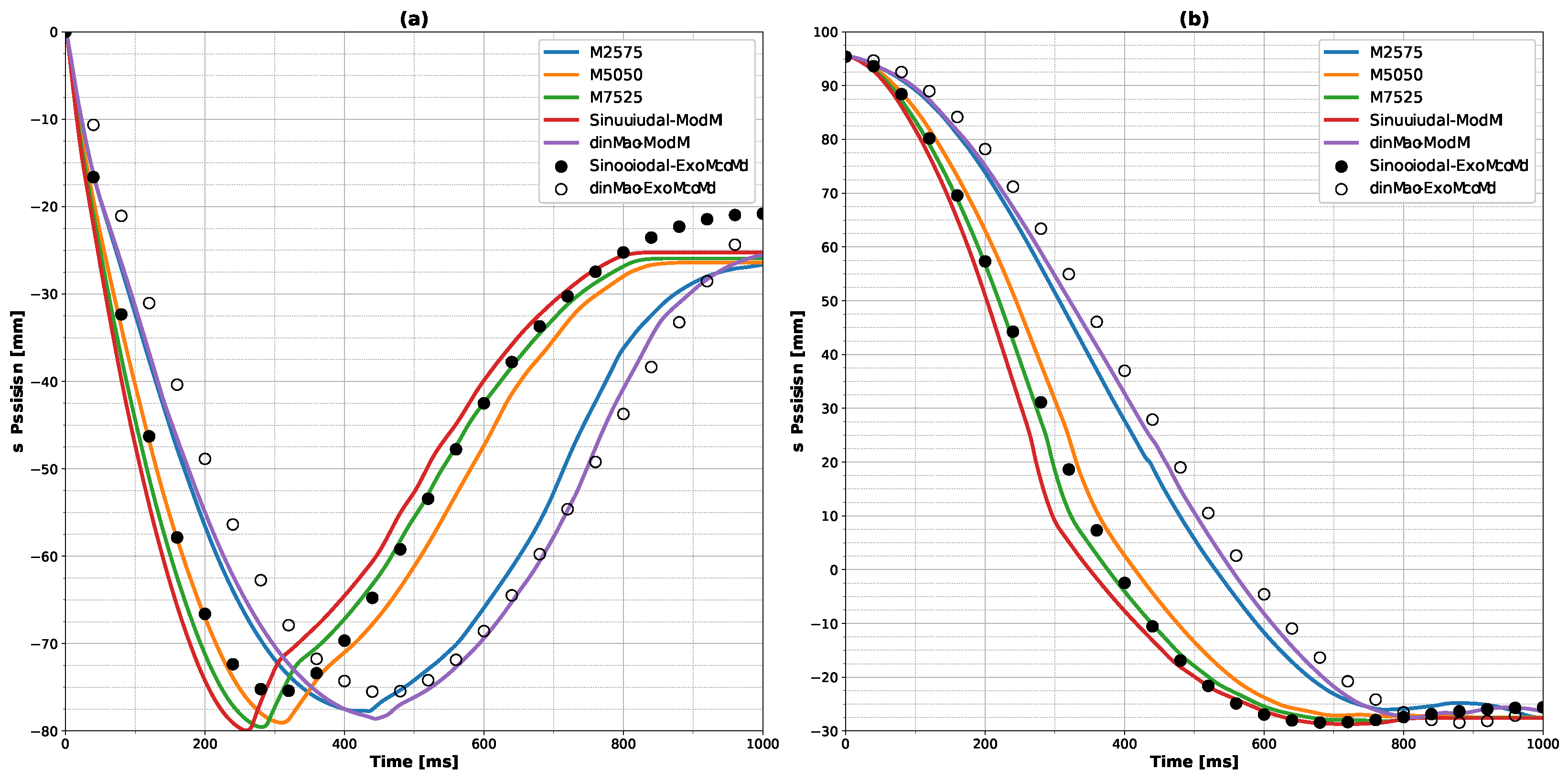
Although this work used a limited amount of data in an attempt to develop a generalized controller for upper limb prostheses, our ANN model was able to make adjustments during the execution of a simple finger movement, and could be extrapolated to more complex movements performed by prostheses. Furthermore, regarding the use of our strategy to develop a controller for upper limb prostheses, it can be seen that there is the possibility for the user to change the inputs, and, consequently, adapt the trajectory, without the need for retraining or online training, as illustrated by changing the linear input for the M2575 combination (Figure 6 and Figure 9). This emphasizes a greater adaptability to and unique control regarding the user’s needs. The main challenge of using an sEMG-based controller can be overcome, that is, the user training process, which is difficult and not very encouraging for amputees. It requires several training sessions, even though pattern classifiers provide high accuracy and virtual training can be used, as shown by Leccia et al. [44]. Using our premises to train a prosthesis controller, we were able to show the possibility of the user changing the inputs, and consequently, the trajectory could be adjusted; for example, the input trajectory could be changed from purely linear to M2575 (Figure 9), providing more adaptability and a unique potential for control, which the user needs. This possibility could facilitate the training process, since the user has the ability to generate their own individual strategies for combining trajectories.

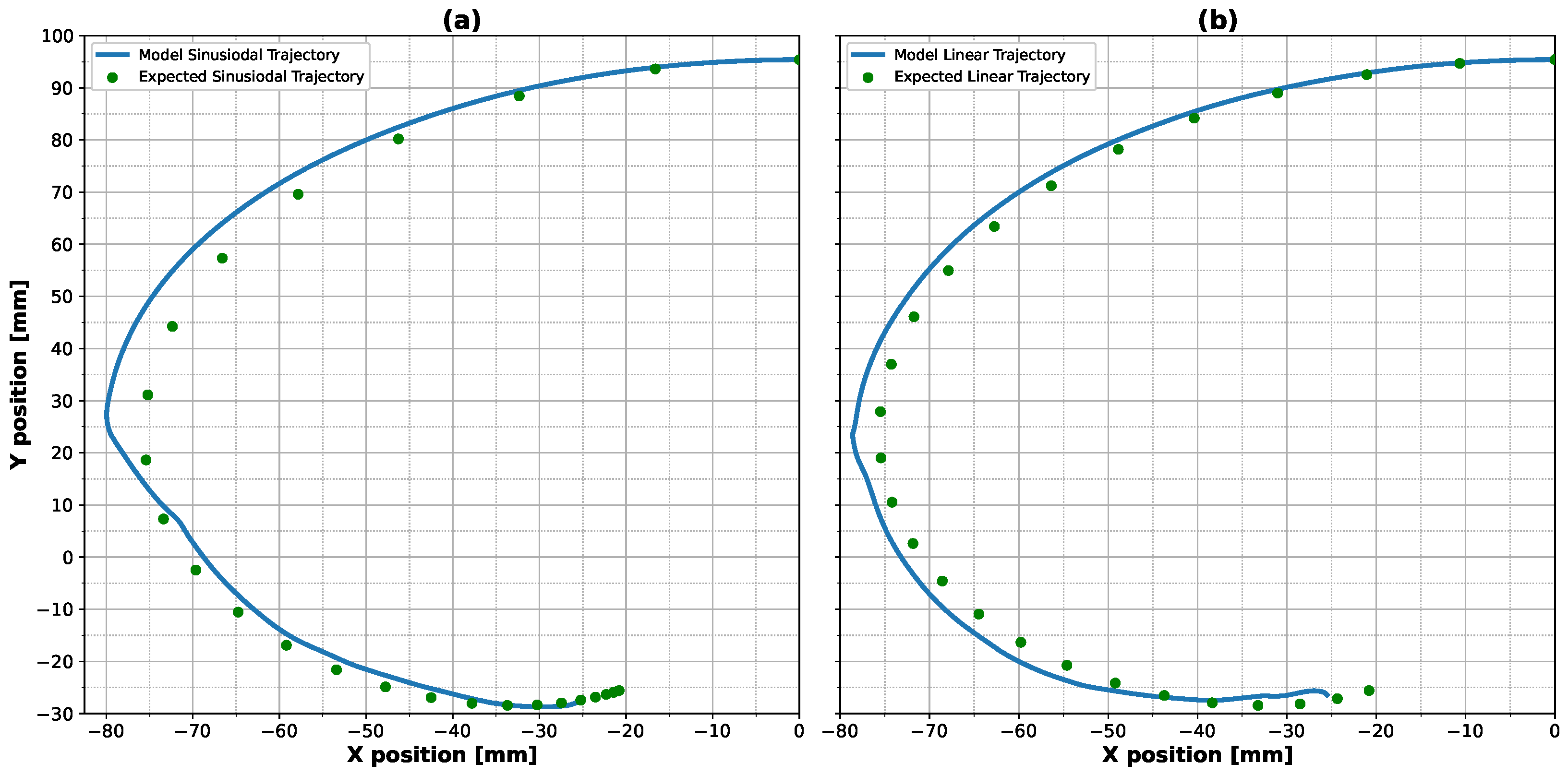
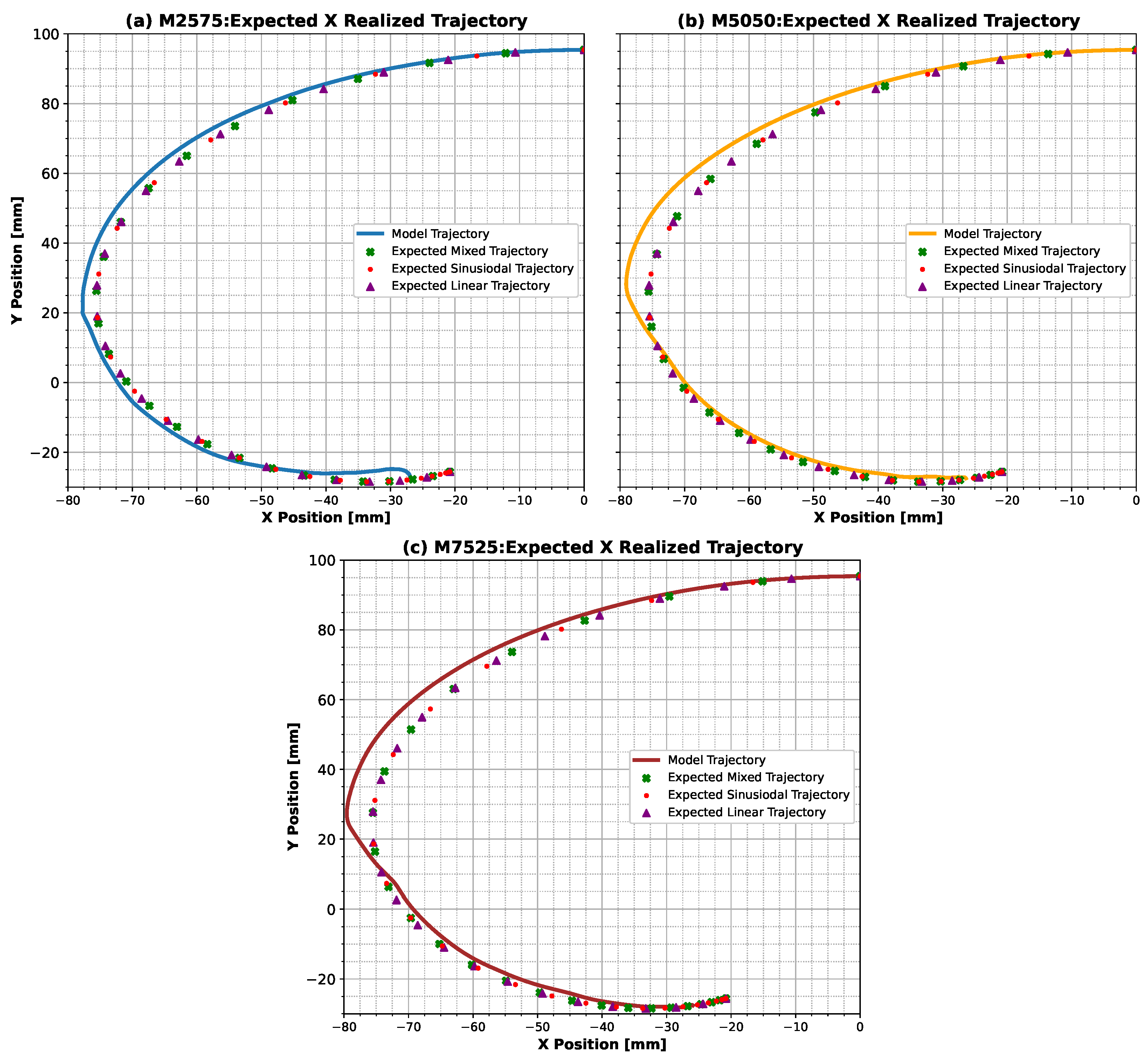
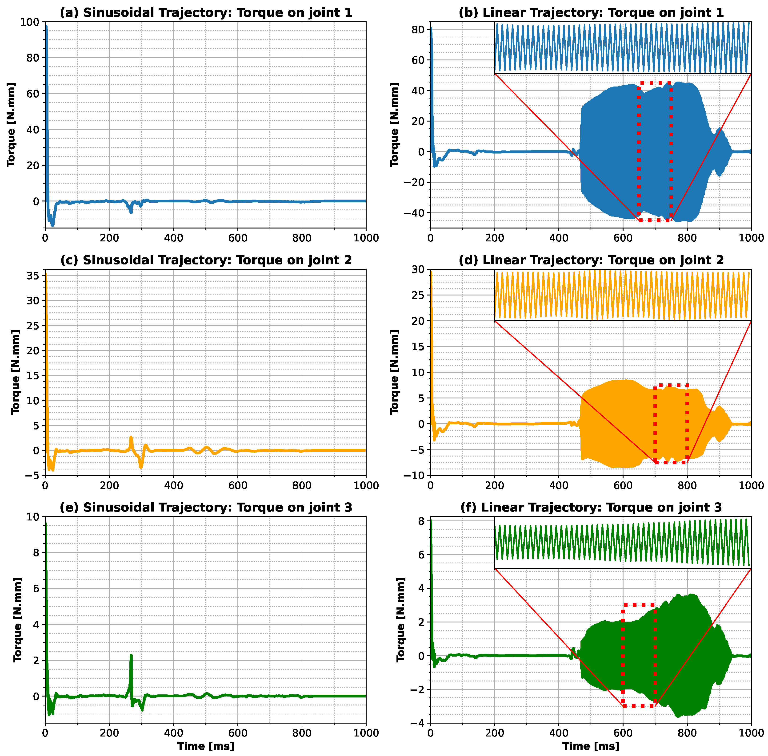
Analyzing the results of the ANN model, it was observed that the different strategies adopted for each case evaluated occurred after the point of maximum distance on the X axis (Figure 2). The main noticeable difference was the oscillatory behavior for the linear case and for the M2575 combination (higher proportion of linear input). In addition, comparing the torque (Figure 3 and Figure 7) with the position with time (Figure 9), we noticed that the points coincided with the abrupt change in the slope of the X component of the trajectory (X component of velocity). This may indicate that the ANN model developed is sensitive to these sudden changes in the kinematic quantities of the finger’s motion. 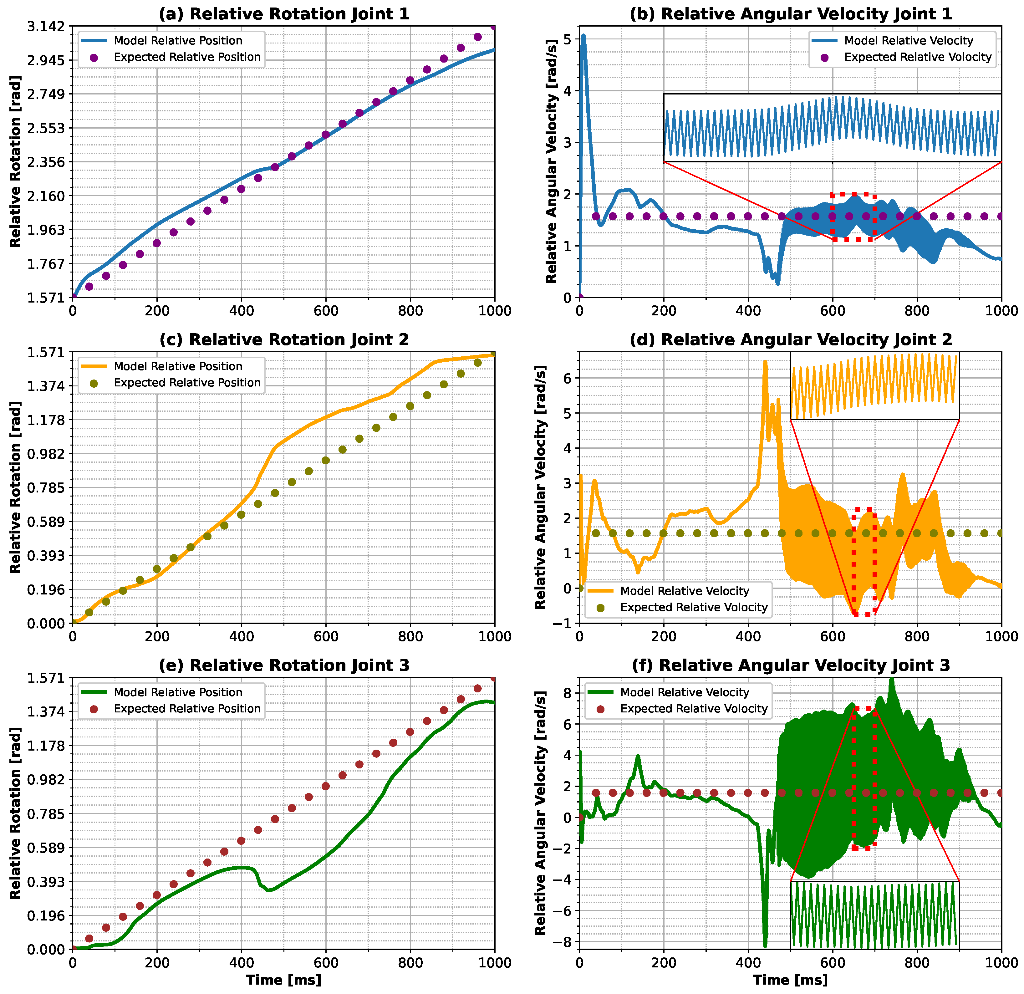Another observation that can be noticed in Figure 2a is the distribution of trajectory points over time. For the sinusoidal trajectory, the density of points changes over time, with more points in the final stages of the motion (showing less error at this stage). The linear trajectory, on the other hand, has a more uniform density of points (showing less error when X is maximum). This difference in the distribution of the points is due to the velocity expected for each trajectory, which explains why the control strategy for the sinusoidal trajectory is more stable. As the finger approaches the end of the movement, the velocity tends toward zero, resulting in a decreasing torque. On the other hand, in the linear trajectory, the velocity is constant throughout the movement, so, to maintain this velocity, it is necessary to constantly stimulate the movement, which causes instability in the control signal. In this case, the proposed controller is more capable of capturing abrupt changes in the position slope and the density of points along the trajectory, demonstrating the ability to differentiate between the features of different trajectories.

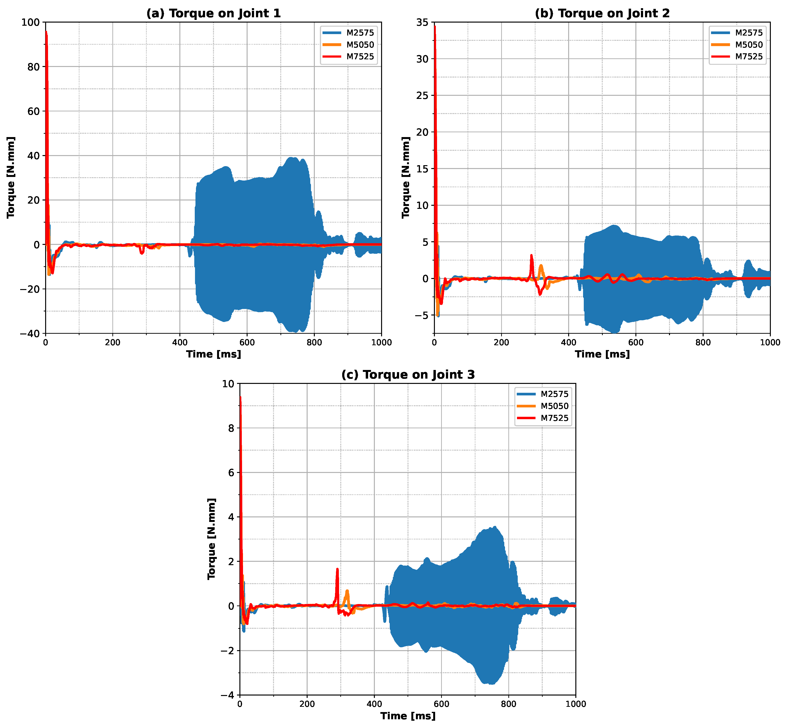
Examining the physics of the problem, it can be observed that the ANN model was able to correctly capture the behavior of the system studied. In the first step, it can be noticed that the peak of the velocity and torque distribution (Figure 3, Figure 4, Figure 5, Figure 7 and Figure 8) was produced to move the finger from the stationary position to the first desired position. After this state, the torque was inverted, however with a less expressive value, since the finger had already started to move. Figure 3 and Figure 7 show that the torque was almost zero during all times until the maximum absolute X distance, at which moment the control strategies were changed. 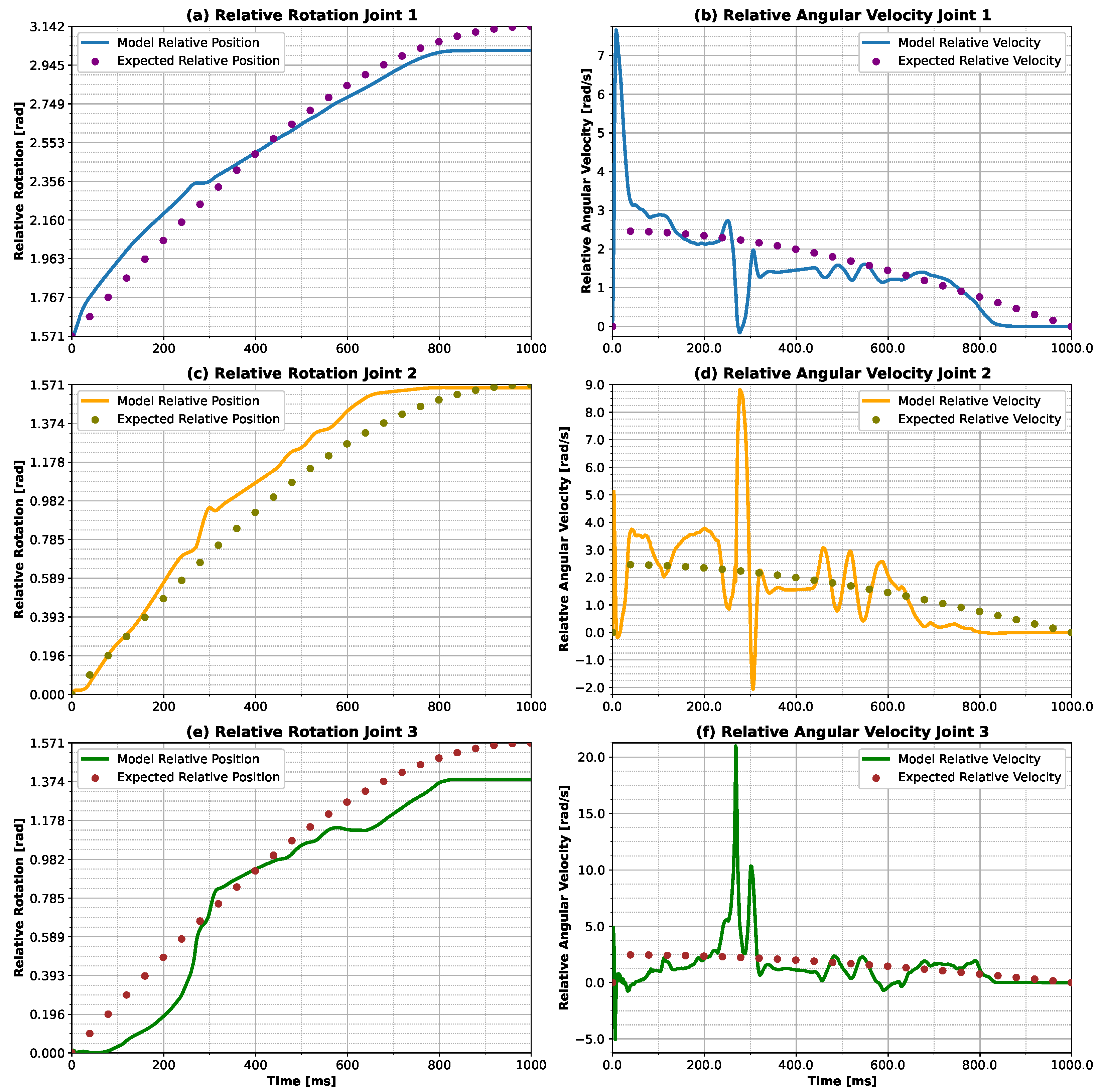One hypothesis to explain this behavior is the application of a higher torque to reverse it, taking advantage of the body’s inertial forces to perform the motion, by the ANN model when a negative slope is developed for the X component of the position (Figure 9a). However, when the slope was positive, the behavior was different for the linear trajectory, which required a constant reversion. The difference may be due to the velocity, which for the sinusoidal trajectory was decreasing as a cosine function, while for the linear trajectory, it was constant. 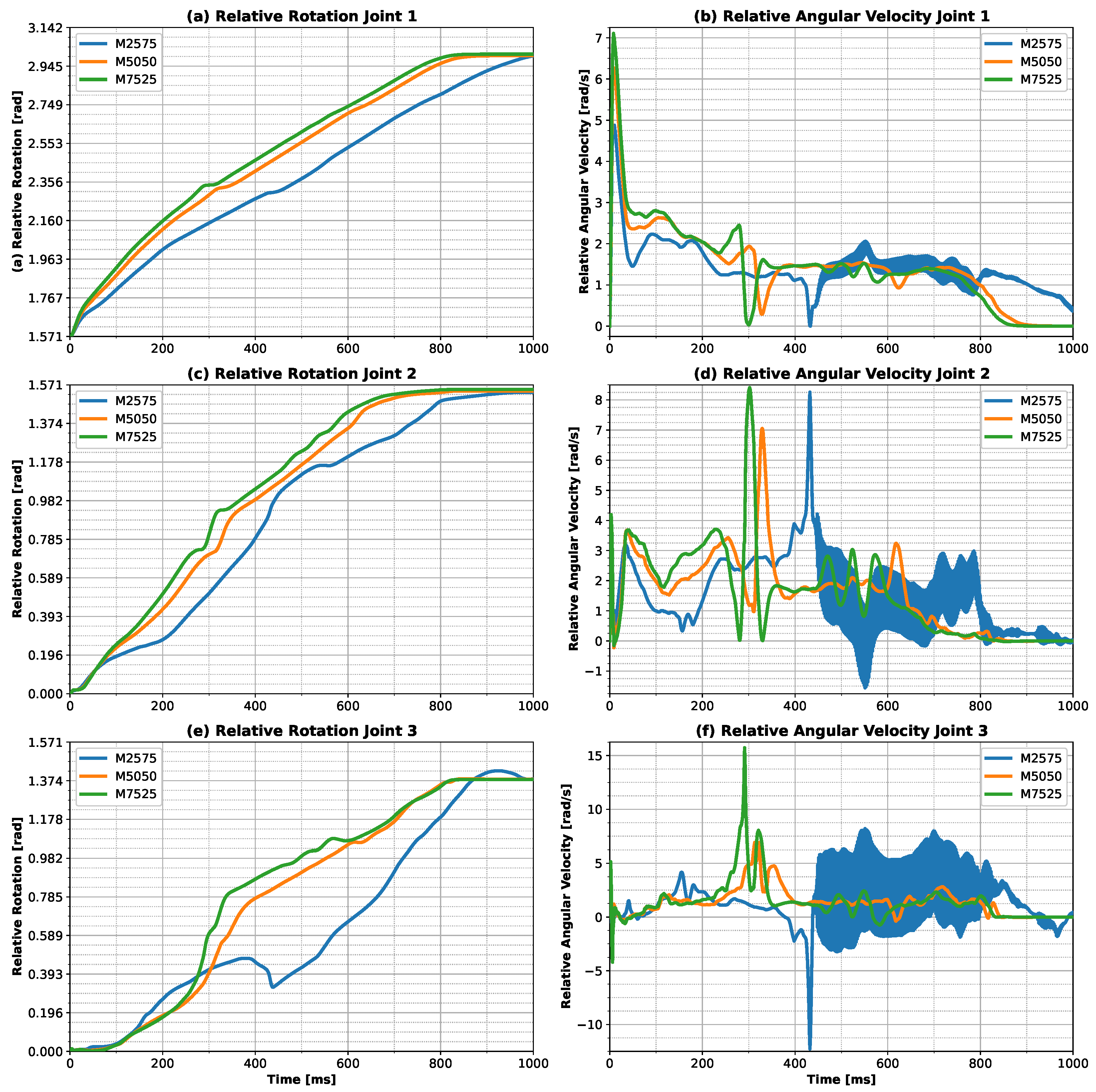For the sinusoidal situation, the positions showed greater difficulty in reaching the desired final positions (Figure 4, Figure 5 and Figure 8). This was caused by the distribution of points, as discussed earlier. For the linear input, the points were equally spaced without changing the velocity magnitude. In contrast, with the sinusoidal trajectory, the spacing between the points was reduced in the final stages, at the same time that the velocity approached zero, making it difficult for the model to reach the desired points at the end of the motion. Another hypothesis that can be formulated is that the controller utilizes both inertia and the desired velocity to formulate the control strategy. 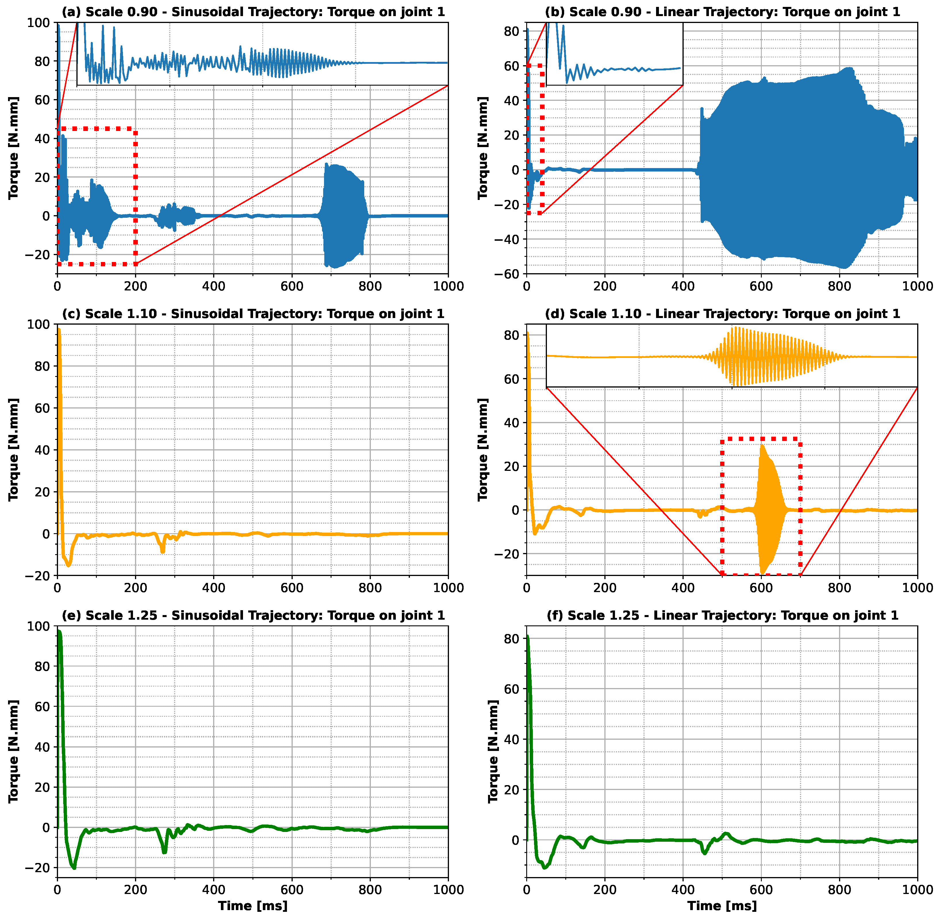This hypothesis can be substantiated by the findings presented in Figure 10, which illustrate the influence of inertia on the control strategy. The analysis reveals that for the larger finger, i.e., with greater inertia, the strategy used for both trajectories was more stable, whereas for the smaller body, i.e., with less inertia, the control strategies were unstable. Considering the situations where different combinations of linear and sinusoidal trajectories were applied (Figure 7), it was possible to see a non-linear relationship established by our ANN model, since no proportionality was observed in the torques. This can be seen from the results obtained for the M5050 case, which was closer to the response for the sinusoidal trajectory than for the other combinations considered (M2575 and M7525).

Finally, by examining the position of the fingertip over time (Figure 9), it was possible to see that the influence on the trajectory error occurred due to the increase in the absolute distance in X between the fingertip and the inertial coordinate axis. One hypothesis to explain this behavior is the increase in torque that the fingertip is subjected to in these positions, generating less stability for the controller, and, consequently, greater difficulty in maintaining the position. The correction that the ANN model chose to avoid the increase in the error in the trajectories may have been the action of the ANN’s actor, in the sense of increasing the absolute value of the reward. Another observation that can be made about the corrections that the ANN model performed along the finger motion is the change in slope position, as demonstrated in Figure 9a, where the slope changes from negative to positive. This change can drastically affect the model’s response, given the observed correction. This fact may be related to the model’s inability to reach the X components of the final positions (Figure 9a), since there is a reduction in the magnitude of the slope of the position X component, making it difficult for the model to determine the correct torque, and leading the torque toward zero in the final stage of the motion (Figure 3 and Figure 7).

Limitations

This work presents some limitations; the main limitations involve the environment of the model and the selected trajectories. The model developed assumes that the phalanges are rigid elements, i.e., any type of deformation that the finger could present was disregarded. Despite the application of this simplifying hypothesis, the dynamics of the finger would not be significantly impacted, since the finger presents small deformations during movement. Another limitation of the model is that the phalanges are represented by elliptical cone trunks with a uniformly distributed density. This consideration has the potential to affect the overall dynamics of the finger, since both the geometry and the distribution of mass along the finger can change the position of the system’s center of mass. Refinements should be performed on these characteristics to improve the quality of the dynamic responses of the model developed. Furthermore, the stiffness and damping terms of the joints between the phalanges were disregarded. This choice was made due to the difficulty of defining these terms, as well as their dependence on the individual. These complexities were outside the scope of the present work, which was focused on evaluating only the ANN model’s ability to perform and adapt different trajectories. The insertion of these elements in the model could affect the stability of the responses generated by the ANN, since they insert a resistive torque and energy dissipation components in each of the joints. Despite this limitation, Figure 10 demonstrates the model’s capacity to modify the control strategy when the dimensions and mass of the finger are changed. This finding suggests the model’s potential to adapt the torque applied to each joint in realistic conditions, where the damping and stiffness parameters of the joints are included. It was also observed that the trajectory errors exhibited no significant differences in relation to the original finger, without applying the scales, which reinforces the hypothesis that a controller using the model proposed in this work could perform the tasks in real environments. In addition, the results presented here have not been validated with experimental data to verify the accuracy of the model in predicting the real dynamics of the finger. However, the aim of this work was to assess the model’s ability to adapt the movement of the finger to different conditions, and these limitations do not negatively affect this type of analysis.

While the present study concentrates on the evaluation of the viability of the DDPG in the development of an adaptive controller, it is acknowledged that other algorithms, such as PPO and SAC, could also be evaluated. This is considered to be a limitation of the present study, since the DDPG is sensitive to buffer hyperparameters, learning rate and the initial parameters of the network, which could affect the results presented [31]. It is believed that both algorithms, PPO and SAC, are the best methods for dealing with a large number of samples, since they show faster convergence and overcome the sensitivities present in the DDPG [20,31,32]. Consequently, if the training was performed using these algorithms, the actor would reach a reward greater than -650 more quickly, which would enable the model to reach higher rewards, thereby improving the overall performance of the ANN. One consequence, despite the rapid convergence, would be a tendency for the model to overflow, which could affect the observed adaptive characteristics. It is, therefore, necessary to evaluate the problem with other deep reinforcement learning algorithms in order to ascertain the real capacity of RL-trained ANNs to adaptively control upper limb prostheses. However, despite the limitations in terms of applicability, the developed controller demonstrated its capacity to generate diverse control signals, according to trajectories and environments, as can be seen in Figure 10 and in the Supplementary Materials.

5. Conclusions

In this study, we evaluated the suitability of using the DDPG algorithm to train an ANN model and propose a new adaptive controller for myoelectric prostheses of the upper limb. We intended to show that it was possible to control physiological finger prostheses in different trajectories and adapt them using trajectory selection through a computational model evaluation. The algorithm demonstrated its efficiency in leading the finger along different trajectories, showing an average magnitude error of $3.984\pm 2.899$ mm for sinusoidal input and $3.220\pm 1.419$ mm for linear input. The results revealed that the model developed different control strategies to achieve the trajectories, demonstrating the ability of the model to distinguish the strategy with only changes in the trajectory’s selected input.

Furthermore, it was possible to observe the model’s compatibility in adapting to different types of trajectory inputs that were not contemplated in the training stage. Considering three combinations of linear and sinusoidal trajectory proportions, the model completed the entirety range of motion without any collisions or failures. This may indicate that the model has the ability to adapt according to the user’s requirements.

Finally, this work proposed the development of a controller to be used in association with myoelectric signals, using RL training. By defining different trajectories, it was possible to develop an adaptive control, which could provide users with easier use and training, offering better integration between the prosthesis and the amputee. As future work, we intend to extrapolate the ANN model to cover the complete hand, using physiological trajectories and classification patterns obtained from sEMG.