Experimental Validation of Passive Monopedal Hopping Mechanism

Abstract

Passive dynamic locomotion, which relies solely on the interaction between the body and the environment, is being explored as an energy-efficient method of movement. The authors’ laboratory investigates passive hopping mechanisms that do not require actuators or sensors. In previous studies, it was demonstrated that an asymptotically stable limit cycle exists in the leg dynamics of a passive hopping model with constrained torso posture. In this study, a monopedal passive hopping robot with constrained torso posture was constructed to validate the existence of the limit cycle. The leg dynamics were evaluated by comparing the trajectories of the model and robot. The results revealed that the leg dynamics of the simulation model represent those of the physical robot. Furthermore, robustness to step disturbances confirmed the validity of leg dynamics.

1. Introduction

Animals that move using their legs, such as humans, can move at high speed on level ground but continue to move without losing their posture even on uneven ground. Because such leg-based locomotion is characterized by the ability to continue moving forward while overcoming obstacles, the development of moving robots designed to mimic the structure and movement of legs is underway. Various robots have been developed, including multi-legged robots inspired by animals [1,2,3] and bipedal robots modeled after human locomotion [4,5,6]. Such robots mostly use active control with sensors and actuators. These robots can perform high-precision movements through precise control. On the other hand, legged robots utilizing passive locomotion without active control have also been developed.

Passive locomotion refers to a type of movement that does not require active control of the body, relying solely on the interaction between the body and the surrounding environment for motion. Passive locomotion is natural movement method that is unconsciously used by humans and animals, in which elastic elements inside the legs, such as muscles and tendons, store kinetic energy as elastic energy during the stance phase. This energy can be used for the next leg swing, improving energy efficiency during movement. Thus, by adding animal-like elastic elements to a robotic leg, it is possible to create a robot that can move with high energy efficiency while achieving natural animal-like dynamics, without active control [7,8,9]. In fact, when comparing the energy efficiency of an actively controlled quadruped robot (MIT Cheetah 3), which has been studied by Bledt et al. [10], and a robot utilizing passive locomotion developed by Collins et al. (Cornell Biped) [11] using the Cost of Transport ((energy used)/(weight·distance)), MIT Cheetah 3 had a value of approximately 0.45 to 1.6, whereas Cornell Biped had a value of 0.2. From the perspective of energy efficiency, this indicates that robots utilizing passive locomotion are superior.

Passive locomotion has been the subject of various studies since its proposal by McGeer [12]. Bipedal passive walking robots [13,14,15] and bipedal passive running robots [16], including Raibert [17], have been investigated and developed. However, this study focused on monopedal passive leaping. The method of locomotion by hopping has been investigated extensively owing to its superior robustness against obstacles compared with walking and running [18,19,20]. Research on monopedal hopping robots utilizing highly energy-efficient passive locomotion has also been progressing [21,22,23].

Posture control of the body is a crucial factor for legged mobile robots. For example, by properly controlling the body during movement to prevent vibrations, it is possible to avoid the robot from toppling over or losing its posture, allowing it to continue moving even when external disturbances are applied [24]. Moreover, posture control helps suppress posture collapse, preventing unnecessary energy consumption of the leg actuators and enabling highly energy-efficient locomotion [25,26]. In this way, posture control contributes to improving locomotion stability, robustness against disturbances, and energy efficiency. For posture control of monopedal robots, methods utilizing reaction wheels [27] and Mode-Reactive Template-Based Control [28] have been proposed. However, in this study, the posture of the body in the monopedal robot is constrained to eliminate its influence, allowing for an in-depth investigation of the dynamics of the leg itself.

The previous study by the authors [29] found that, in a monopedal passive hopping model with a constrained body posture, the leg dynamics exhibited an asymptotically stable limit cycle. In this study, a similar monopedal passive hopping robot with a constrained body posture was developed to demonstrate the existence of an asymptotically stable limit cycle in leg dynamics. Furthermore, the validity of leg dynamics was verified by comparing the hopping trajectories of the model and robot.

The Spring-Loaded Inverted Pendulum (SLIP) model [30] is a representative leg model that does not consider torso posture. The SLIP model enables continuous periodic hopping by fixing the landing angle and controlling the torso posture during the stance phase. Since this model exhibits the natural characteristics of animal legs, it has also been applied to the design of robotic legs [31,32]. In this study, we perform parameter selection and design through simulations for a leg model that, like the SLIP model, does not consider torso posture. By demonstrating the existence of an asymptotically stable limit cycle, we consider that this approach can be applied to the design of legged robots based on the SLIP model.

2. Simulation Model

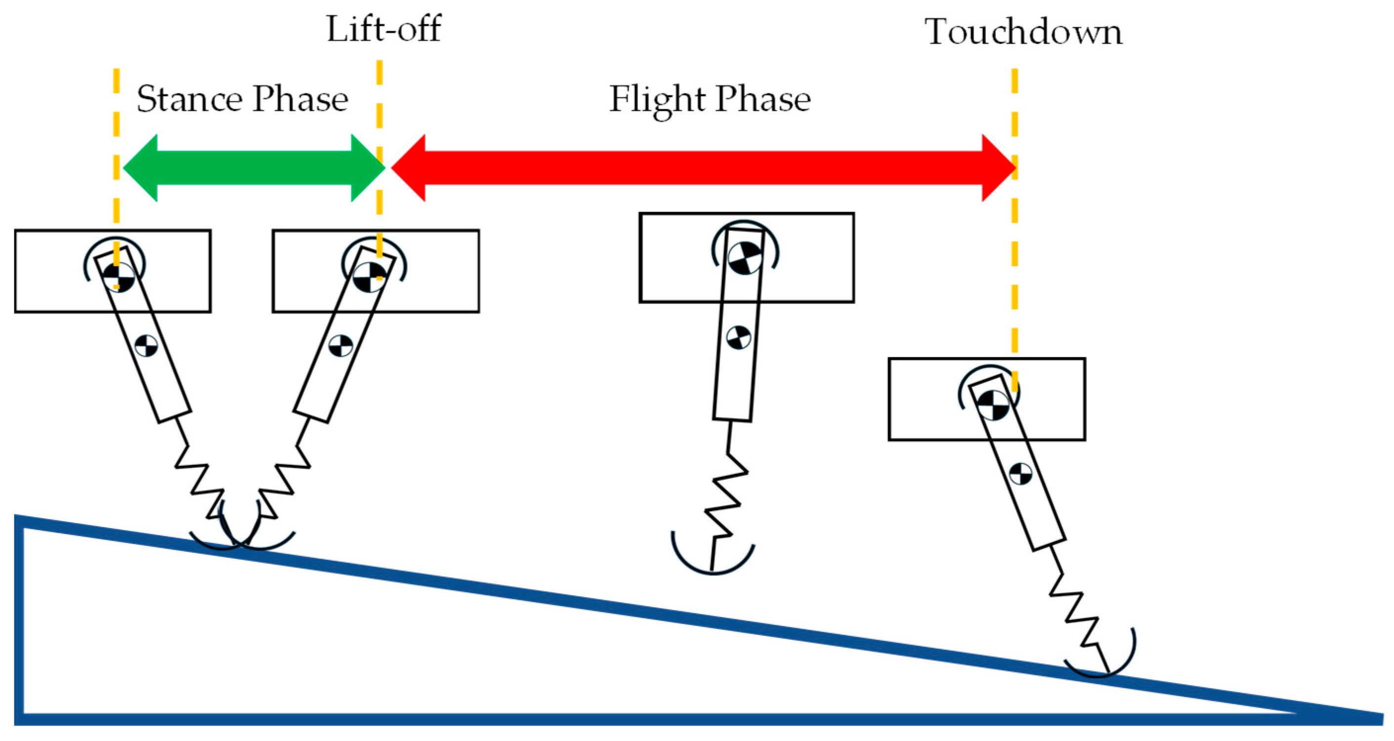
2.1. Monopedal Passive Hopping Model

Figure 1 shows the monopedal passive hopping model used in this study. To investigate the passive dynamics of legs, it is necessary to constrain the body posture of the model. To this end, supporting devices are added to the model to prevent torso rotation and tipping to the left or right. The legs are considered as rigid bodies with a moment of inertia $j_{leg}$, and the centers of gravity of the torso and legs are set at different locations. Compression springs are placed at the legs’ tips; therefore, the leg length changes during movement. Torsion springs are placed between the legs and the torso, allowing the legs to swing freely during hopping. The variables used in this simulation are listed in

Table 1. Variables in simulation model.

Symbol	Description
$m_b$[kg]	Body mass
$m_l$[kg]	Leg mass
$m_e$[kg]	Supporting device mass
$k_l$[N/m]	Spring constant of leg
$k_h$[Nm/rad]	Spring constant of hip
$j_{leg}$[Nm2]	Leg moment of inertia
$c_l$[Ns/m]	Damping constant of leg
$c_h$[Ns/rad]	Damping constant of hip
$c_{ex}$[Ns/m]	Horizontal Damping constant of Supporting device
$c_{ey}$[Ns/m]	Vertical Damping constant of Supporting device
$a$[m]	Distance from the center of mass of the leg to the center of arc of the toes
$b$[m]	Distance from hip joint to center of mass of leg
$r_0$[m]	$\mathrm{Natural} \mathrm{leg} \mathrm{length} (a+b$)
$r$[m]	Leg length
$r_f$[Nm2]	Arc radius of the toe
$\alpha$[deg]	Angle of inclination
$x$[m]	Horizontal displacement of the hip joint
$y$[m]	Vertical displacement of the hip joint
$x_l$[m]	Horizontal displacement of leg center of mass
$y_l$[m]	Vertical displacement of leg center of mass

.

2.2. Methods of Model Analysis

The model hops by repeating the stance and flight phases, as shown in Figure 2. The model in the stance and flight phases moves according to the equations of motion, and the state of each phase transitions by lift-off and touchdown. The equations of motion, lift-off, and touchdown in each phase are presented in the following sections.

2.2.1. Equation of Motion for Stance Phase

The equations of motion for the stance phase were derived from the Euler–Lagrange equations. The Lagrangian used in the derivation is expressed by Equation (1) and the dissipation function is expressed by Equation (2).

$$L={\displaystyle \frac{1}{2}}{m}_b\left({\dot{x}}^2+{\dot{y}}^2\right)+{\displaystyle \frac{1}{2}}J{\dot{\theta }}^2-{\displaystyle \frac{1}{2}}{k}_l{\left(r-r_0\right)}^2-{\displaystyle \frac{1}{2}}{k}_h{\theta }^2-m_{b}gy+{\displaystyle \frac{1}{2}}{m}_l\left({{\dot{x}}_l}^2+{{\dot{y}}_l}^2\right)+{\displaystyle \frac{1}{2}}{m}_l{b}^2{\dot{\theta }}^2-m_{l}g{y}_l-{\displaystyle \frac{1}{2}}{m}_e{\dot{x}}^2,$$

(1)

$$D={\displaystyle \frac{1}{2}}{c}_h{\dot{\theta }}^2+{\displaystyle \frac{1}{2}}{c}_l{\dot{r}}^2+{\displaystyle \frac{1}{2}}{c}_{ex}{\dot{x}}^2+{\displaystyle \frac{1}{2}}{c}_{ey}{\dot{y}}^2.$$

(2)

In the stance phase, the coordinates of the hip joint ($x,y)$ and those of the leg center of mass ($x_l, y_l$) can be expressed as $r, r_f,a,\alpha ,\theta$ by taking the point where the toes touch the ground as the origin. The equations for ($x, y)$ and ($x_l,y_l$) are expressed by Equations (3)–(6).

$$x=r_f\left({\theta }_{td}-\theta \right)\cos \alpha +r_f\sin \alpha -r\sin \left(\theta -\alpha \right),$$

(3)

$$y=r_f\cos \alpha -r_f\left({\theta }_{td}-\theta \right)\sin \alpha +r\cos \left(\theta -\alpha \right),$$

(4)

$$x_l=r_f\left({\theta }_{td}-\theta \right)\cos \alpha +r_f\sin \alpha -a\sin \left(\theta -\alpha \right),$$

(5)

$$y_l=r_f\cos \alpha -r_f\left({\theta }_{td}-\theta \right)\sin \alpha +a\cos \left(\theta -\alpha \right).$$

(6)

Hence, the equations of motion for the stance phase are expressed by Equations (7) and (8) with the generalized coordinates denoted as [$\theta , r$]. Here, the leg length $r$ changes during the stance phase, and the leg velocity $\dot{r}$ is positive in the direction of leg extension. The definitions of $M,R_c$, and $R_s$ used in Equations (7) and (8) are given in Equations (9)–(11).

$$\begin{array}{c}\left\{M{r}_f^2+m_b{r}^2+m_l{\left(r-b\right)}^2+j_l-m_l{b}^2+2\left(Mr-m_{l}b\right)r_f\cos \theta \right\}\ddot{\theta },\\ =\left\{\left(Mr-m_{l}b\right)r_f\sin \theta -m_{e}r\sin \left(\theta -\alpha \right)R_c\right\}{\dot{\theta }}^2\\ -2\left\{\left(M{r}_f\cos \theta +M_b\right)-m_e\cos \left(\theta -\alpha \right)R_c\right\}\dot{r}\dot{\theta }\\ -\left\{M{r}_f\sin \theta -m_e\sin \left(\theta -\alpha \right)R_c\right\}\ddot{r}\\ -k_h\theta -M{r}_{f}g\sin \alpha +\left(Mr-m_{l}b\right)g\sin \left(\theta -\alpha \right)\\ -c_h\dot{\theta }-c_{ex}{R}_c\left(R_c\dot{\theta }+\dot{r}\sin \left(\theta -\alpha \right)\right)-c_{ey}{R}_s\left(R_s\dot{\theta }+\dot{r}\cos \left(\theta -\alpha \right)\right)\end{array}$$

(7)

$$\begin{array}{c}\left\{M{r}_f\sin \theta -m_e\sin \left(\theta -\alpha \right)R_c\right\}\ddot{\theta }\\ =\left\{\left(Mr-m_{l}b\right)-m_{e}r{\sin }^2\left(\theta -\alpha \right)\right\}{\dot{\theta }}^2\\ +\left(m_e\sin 2\theta \right)\dot{r}\dot{\theta }\\ -\left\{M-m_e{\sin }^2\left(\theta -\alpha \right)\right\}\ddot{r}\\ -k_l\left(r-r_0\right)-Mg\cos \left(\theta -\alpha \right)-c_l\dot{r}\\ -c_{ex}\sin \left(\theta -\alpha \right)\left(\dot{r}\sin \left(\theta -\alpha \right)+R_c\dot{\theta }\right)-c_{ey}\cos \left(\theta -\alpha \right)\left(\dot{r}\cos \left(\theta -\alpha \right)+R_s\dot{\theta }\right),\end{array}$$

(8)

$$M=m_b+m_l,$$

(9)

$$R_c=r_f\cos \alpha +r\cos \left(\theta -\alpha \right),$$

(10)

$$R_s=r_f\sin \alpha -r\sin \left(\theta -\alpha \right).$$

(11)

2.2.2. Equation of Motion for Flight Phase

Similarly, the equations of motion for the flight phase were derived from the Euler–Lagrange equations. The Lagrangian used in the derivation is expressed by Equation (12) and the dissipation function is expressed by Equation (13).

$$\begin{array}{c}L={\displaystyle \frac{1}{2}}{m}_b\left({\dot{x}}^2+{\dot{y}}^2\right)+{\displaystyle \frac{1}{2}}J{\dot{\theta }}^2-{\displaystyle \frac{1}{2}}{k}_l{\left(r-r_0\right)}^2-{\displaystyle \frac{1}{2}}{k}_h{\theta }^2-m_{b}gy+{\displaystyle \frac{1}{2}}{m}_l\left({{\dot{x}}_l}^2+{{\dot{y}}_l}^2\right)\\ +{\displaystyle \frac{1}{2}}{m}_l{b}^2{\dot{\theta }}^2-m_{l}g{y}_l-{\displaystyle \frac{1}{2}}{m}_e{\dot{x}}^2,\end{array}$$

(12)

$$D={\displaystyle \frac{1}{2}}{c}_h{\dot{\theta }}^2+{\displaystyle \frac{1}{2}}{c}_l{\dot{r}}^2+{\displaystyle \frac{1}{2}}{c}_{ex}{\dot{x}}^2+{\displaystyle \frac{1}{2}}{c}_{ey}{\dot{y}}^2.$$

(13)

The equations of motion for the flight phase are defined in Equations (14)–(16) with the generalized coordinates [$x,y,\theta$].

$$\left(M-m_e\right)\ddot{x}=-m_{l}b\cos \left(\theta -\alpha \right)\ddot{\theta }+m_{l}b\sin \left(\theta -\alpha \right){\dot{\theta }}^2-c_{ex}\dot{x},$$

(14)

$$M\ddot{y}=-m_{l}b\sin \left(\theta -\alpha \right)\ddot{\theta }-m_{l}b\cos \left(\theta -\alpha \right){\dot{\theta }}^2-Mg-c_{ey}\dot{y},$$

(15)

$$j_l\ddot{\theta }+m_{l}b\cos \left(\theta -\alpha \right)\ddot{x}+m_{l}b\sin \left(\theta -\alpha \right)\ddot{y}=-k_h\theta -m_{l}bg\sin \left(\theta -\alpha \right)-c_h\dot{\theta }.$$

(16)

2.2.3. Lift-Off

The model performs lift-off when transitioning from the stance phase to the flight phase. Lift-off occurs when the leg length $r$ returns to its natural leg length $r_0$ during the stance phase and the leg velocity $\dot{r}$ is positive, as follows:

$$r=r_0,$$

(17)

$$\dot{r}>0.$$

(18)

2.2.4. Touchdown

• When the model deviates from the flight phase to the stance phase, a collision occurs between the model’s feet and the ground. During this collision, the leg tips do not slide and the collision is assumed to be fully inelastic.
• The following equations can be considered, based on the law of momentum conservation in the legs and the law of angular momentum conservation around the hip joint and touchdown point before and after collision:

  $${\mathit{Q}}^{-}{\left[{\dot{\theta }}^{-},{\dot{x}}^{-},{\dot{y}}^{-}\right]}^T={\mathit{Q}}^{+}{\left[{\dot{\theta }}^{+},{\dot{r}}^{+}\right]}^T,$$

  (19)

  where ${\left[{\dot{\theta }}^{-},{\dot{x}}^{-},{\dot{y}}^{-}\right]}^T$ and ${\left[{\dot{\theta }}^{+},{\dot{r}}^{+}\right]}^T$ represent the state vector immediately before and after touchdown, respectively. Therefore, the states immediately before and after touchdown are derived by Equations (19)–(21).

  $${\left[{\dot{\theta }}^{+},{\dot{r}}^{+}\right]}^T={\left({\mathit{Q}}^{+}\right)}^{-1}{\mathit{Q}}^{-}{\left[{\dot{\theta }}^{-},{\dot{x}}^{-},{\dot{y}}^{-}\right]}^T,$$

  (20)

  $${\mathit{Q}}^{-}={\left[\begin{array}{cc}{J}_l+J_l{\displaystyle \frac{r_f}{r_0}}\cos {\theta }_s^{-}-m_{l}b\left(a+r_f\mathit{cos}{\theta }_s^{+}\right)& 0\\ -\left\{m_b{r}_0+m_{l}a\right\}\cos \left({\theta }_s^{-}-\alpha \right)-M{r}_f\cos \alpha +m_e{R}_c& -(M-m_e)\sin \left({\theta }_s^{-}-\alpha \right)\\ -\left\{m_b{r}_0+m_{l}a\right\}\sin \left({\theta }_s^{-}-\alpha \right)+M{r}_f\sin \alpha & M\cos \left({\theta }_s^{-}-\alpha \right)\end{array}\right]}^T,$$

  (21)

  $${\mathit{Q}}^{+}={\left[\begin{array}{cc}\left(m_b+{\displaystyle \frac{J_l}{r_0^2}}\right)\left(r+r_f\cos {\theta }_s^{+}\right)r+m_{l}a\left(a+r_f\cos {\theta }_s^{+}\right)& 0\\ \left(M+{\displaystyle \frac{J_l}{r_0^2}}\right)r_f\sin {\theta }_s^{+}& M\end{array}\right]}^T.$$

  (22)

2.2.5. Stability Analysis

The Poincaré map was used to analyze hopping stability. When a periodic orbit exists in an n-dimensional state space with n ≥ 2, the (n − 1)-dimensional plane S, which is set up to be traversed by the orbit, is called a Poincaré section.

In this study, the Poincaré section was assumed to be immediately after touchdown. The Newton–Raphson method was used to investigate the fixed point where the difference between the initial value in the stance phase of the $k$ step and the initial value in the stance phase of the $k+1$ step approaches zero. The following Poincaré map derives the initial value $x_k={\left[\begin{array}{cc}\begin{array}{ccc}\theta & \dot{\theta }& r\end{array}& \dot{r}\end{array}\right]}_k^T$ in the $k+1$ step phase from the initial value $x_k={\left[\begin{array}{cc}\begin{array}{ccc}\theta & \dot{\theta }& r\end{array}& \dot{r}\end{array}\right]}_k^T$ in the $k$ step phase.

$$x_{k+1}=\mathit{P}\left(x_k\right),$$

(23)

where $x_f$ is a fixed point:

$$x_f=\mathit{P}\left(x_f\right)$$

(24)

By linearizing around this fixed point, the Jacobian ${\mathit{J}}_{\mathit{f}}$ of the Poincaré map is derived.

$$∆x_{k+1}={\mathit{J}}_{\mathit{f}}∆x_k$$

(25)

In this study, the initial value is the fixed point when the difference between all variables within $x_k$ and $x_{k+1}$ is less than ${10}^{-6}$. A hop is considered stable when the eigenvalue of the Jacobian ${\mathit{J}}_{\mathit{f}}$ is less than 1.

3. Monopedal Passive Hopping Robot

3.1. Monopedal Passive Hopping Robot Concept

This section describes the concept of the actual passive hopping robot. The robot is shown in Figure 3. The main body of the robot has a torsion spring attached to the hip joint, Figure 3a, and a compression spring attached to the leg, Figure 3b. Linear bushings, Figure 3c, and ball splines, Figure 3d, were used to connect the supporting devices to each other and to the hopping robot, respectively. These supporting devices allow the hopping robot to move up and down and back and forth, but the devices are constrained to prevent the robot from falling over and rotating. Without considering the supporting device fixed to the ground, the mass of the robot is 4.33 kg, its height is 0.5 m, and its width is 0.68 m.

3.2. Hip Spring

Hip springs are used to connect the leg and body at the hip joint. During the stance phase and flight phase, the leg oscillates like a pendulum under the influence of force, as shown in Figure 4a. By changing the spring constant $k_h$ of the hip spring, the period of leg oscillation can be changed, and the hopping speed and period can be adjusted. In this study, the spring has $k_h$ = 3.17 Nm/rad and is connected in parallel to two crotch nodes.

3.3. Leg Spring

A compression spring is attached to the leg tip. During the stance phase, as shown in Figure 4b, an external force acts on the springs to store energy inside the leg springs, enabling the robot to hop. In this study, the leg springs have $k_l$ = 2.04 N/mm and are connected in parallel to the leg tips.

3.4. Linear Bushing

The supporting device fixed to the ground and the supporting device connected to the main body of the hopping robot are connected to each other using a linear bush (MISUMI from Japan, model number: SC16UU) as shown in Figure 4c. The linear bush uses the rolling motion of the balls inside the bearing, which are in point contact with the shaft to achieve low-friction, high-precision linear motion. The linear bushes are attached to the left and right sides of the supporting device to enable the smooth vertical movement of the hopping robot’s main body.

3.5. Ball Splines

A ball spline (MISUMI from Japan, model number: BSJM10-600-F20-E20-P8-Q8-NTW) is used for the connection between the supporting device and the body of the hopping robot, as shown in Figure 4d. When an external force is applied to the ball spline, the ball inside the outer cylinder, called the spline nut, rolls along the ball groove of the spline shaft, enabling high-precision linear motion. The ball spline enables the main body to move freely in the forward and backward directions while maintaining constant body posture.

3.6. Hopping Mechanism

Figure 4e and Figure 5 show the robot’s movements during hopping. After lift-off, the robot stores energy by contracting the leg springs during the stance phase and simultaneously pushes the body forward by swinging the legs backward. The robot takes off when the contracted leg springs return to their natural length, and the legs are swung forward by the hip springs during the flight phase. The legs swing forward to contact the ground, returning the hopping to its initial state. The robot continues to hop by repeating this action.

The model and robot developed in this study are based on limit cycle walking/hopping for the locomotion of legged robots [33]. Limit cycle walking/hopping has higher energy efficiency during locomotion compared to actively controlled robots. In fact, the legged robot developed by Longchuan et al. [34] was able to improve energy efficiency during locomotion by utilizing passive walking/hopping based on a limit cycle. Similarly, in this study’s model, the inherent limit cycle of leg dynamics suggests the possibility of addressing the challenge of energetic efficiency during locomotion.

Moreover, even if the model and robot in this study deviate from the periodic trajectory due to external disturbances during hopping, the asymptotically stable limit cycle inherent in the leg dynamics allows them to return to the original trajectory without any external control. In actively controlled robots, a high feedback gain is required to bring the system back to the trajectory when it deviates, leading to increased energy consumption. In contrast, robots based on limit cycle walking/hopping do not require feedback gain, enabling them to continue hopping while maintaining high energy efficiency even when disturbances are applied [33] (p. 288).

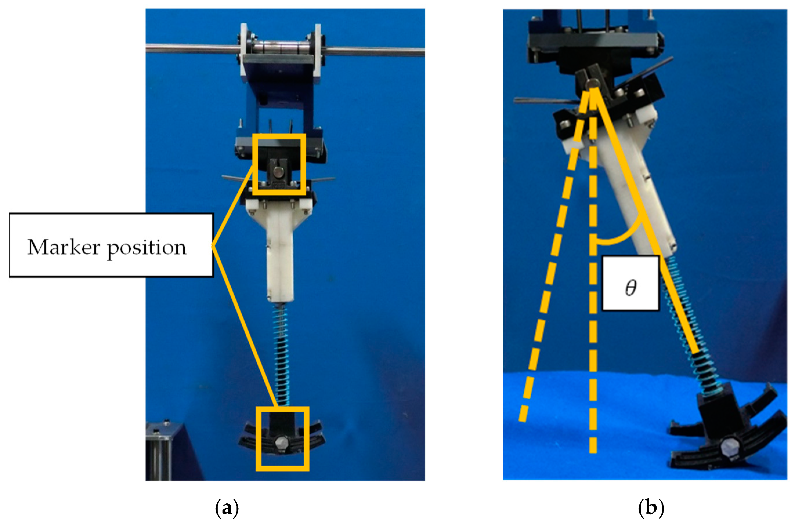
3.7. Passive Hopping Robot Analysis Method

The movement of the hopping robot was analyzed using two-dimensional video analysis software (PV studio 2D, ver. 2; L.A.B. Co). In this study, markers were placed at the hip joint and leg tips, as shown in Figure 6a. The hopping robot was tested by performing hops on a treadmill, and the leg angle and movement amount were measured by detecting the marker coordinates at the time of the hop. The leg angle $\theta$ was set to 0° when the leg was perpendicular to the ground. When the legs are forward, as shown in Figure 6b, $\theta$ takes a positive value; when the legs are swinging backward, $\theta$ takes a negative value.

4. Comparison Between Measurement Results for Hopping Robot and Simulation Results

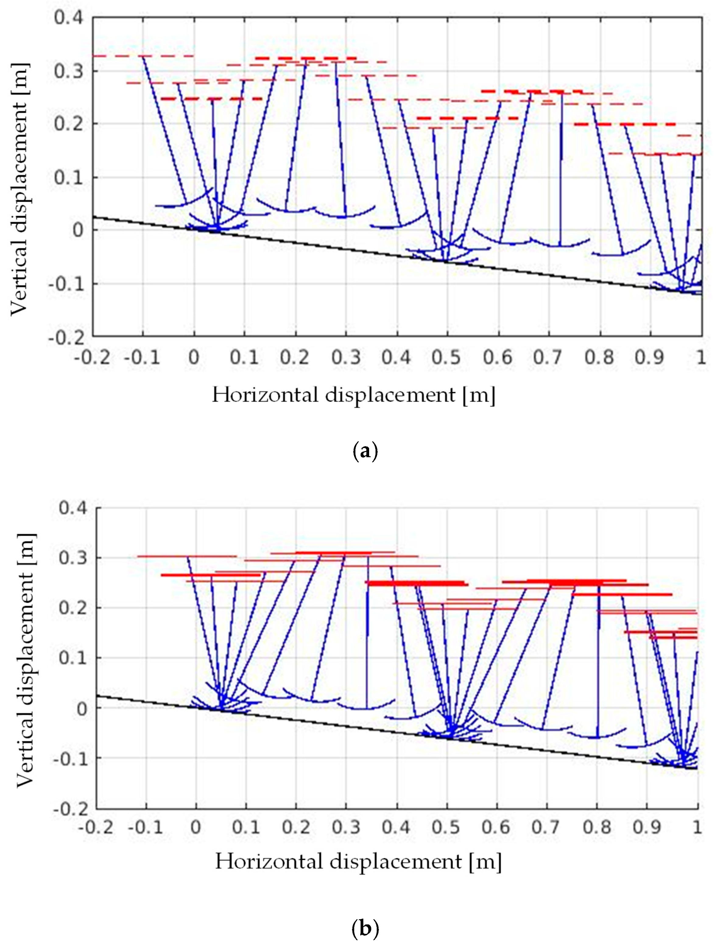
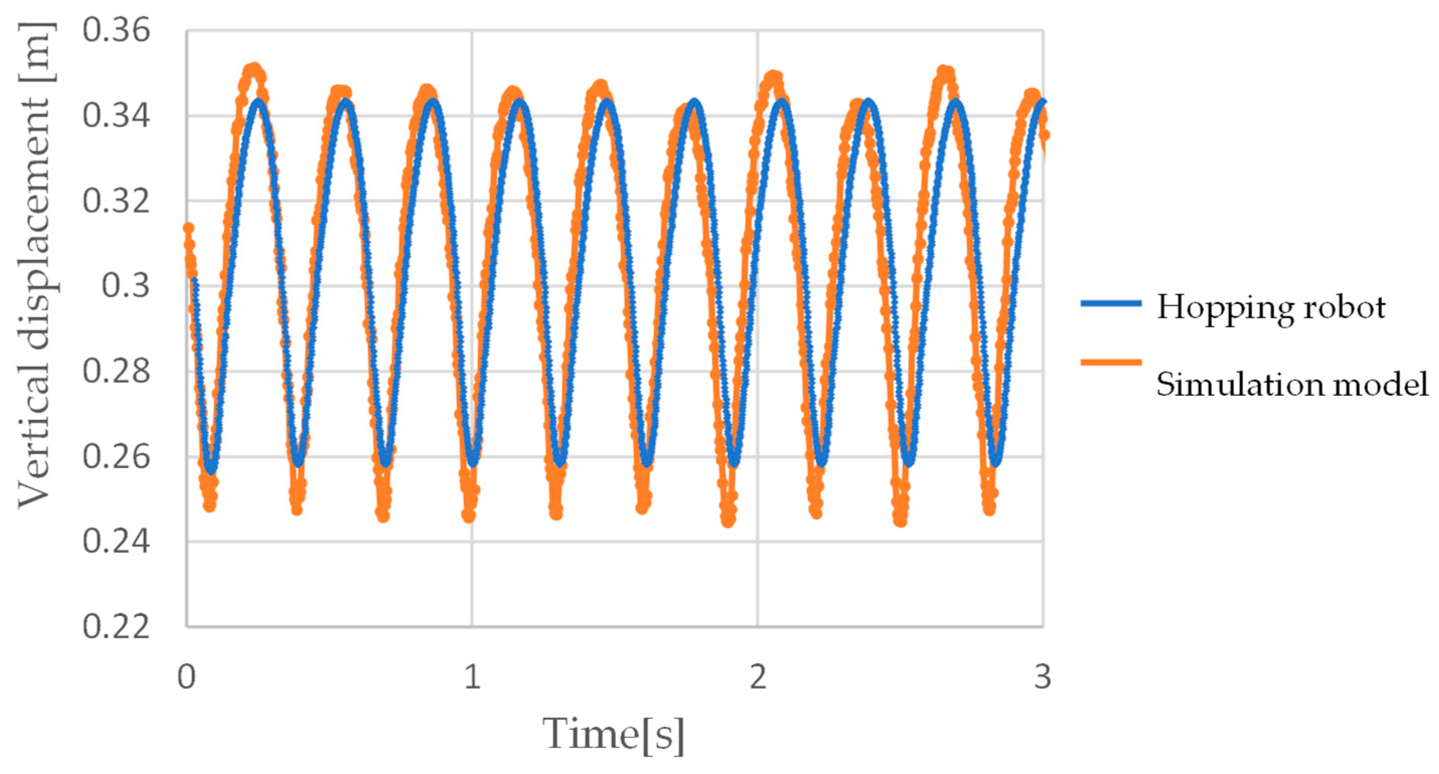
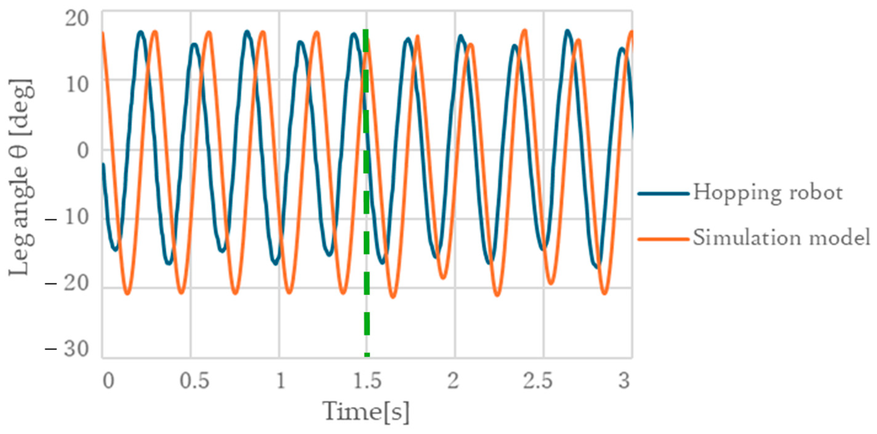
4.1. Comparison of Actual and Simulated Trajectories

In this section, the results obtained from the numerical simulation are compared with the trajectories of the hopping robot. The hopping physical parameters obtained from the simulation are shown in

Table 2. Physical parameters of simulation model and hopping robot.

Symbol	Description	Value
$m_b$[kg]	Body mass	3.5
$m_l$[kg]	Leg mass	0.83
$m_e$[kg]	Supporting device mass	1.49
$k_l$[N/m]	Spring constant of leg	4080
$k_h$[N/rad]	Spring constant of hip	6.34
$j_l$[Nm2]	Leg moment of inertia	9.36 × 10−3
$c_l$[Ns/m]	Damping constant of leg	5.0
$c_h$[Ns/rad]	Damping constant of hip	0.04
$c_{ex}$[Ns/m]	Horizontal Damping constant of Supporting device	2.0
$c_{ey}$[Ns/m]	Vertical Damping constant of Supporting device	0.1
$a$[m]	Distance from the center of mass of the leg to the center of arc of the toes	0.100
$b$[m]	Distance from hip joint to center of mass of leg	0.085
$r_0$[m]	$\mathrm{Natural} \mathrm{leg} \mathrm{length} (a+b$)	0.185
$r_f$[Nm2]	Arc radius of the toe	0.12
$\alpha$[deg]	Angle of inclination	7

, and one cycle of the hopping motion on a treadmill with a speed of 5.4 m/s is illustrated in Figure 7. The physical parameters in this study were selected to ensure that the eigenvalue of the Poincaré map is 0.87, indicating the presence of an asymptotically stable limit cycle. The red dots in Figure 7 represent the marker positions used in PV Studio 2D. The hopping trajectory derived from these marker positions and the simulation’s hopping trajectory are presented in Figure 8. Comparisons of the temporal variations of the leg angle $\theta$ and the vertical displacement y during hopping are shown in Figure 9 and Figure 10, respectively.

Figure 9 shows that the hopping cycles of the simulation and robot are similar. Over 20 hops, the difference in the cycle duration per step reveals that the simulation hops are marginally shorter by 3.21 $\times {10}^{-3}$s. The amount of change in the angle shows that, in the simulation, the legs are more forward compared with those of the robot. When averaged over 20 steps, the simulated leg swung forward by 5.37°. As shown in Figure 10, the vertical displacements of the hip joints of the actual and simulated robot are close. By comparing the values for 10 steps, it can be found that the average simulation displacement is 0.012 m greater than that of the robot. Figure 11 is a phase portrait with the leg angle on the horizontal axis and the leg angular velocity on the vertical axis. From this phase portrait, closed orbits were observed in both the simulation model and the hopping machine, confirming the presence of a limit cycle in both systems.

These results confirm that the differences between the simulation and the hopping robot in both the leg angle and the vertical displacement are small, and that the hopping trajectories of the hopping robot and simulation are qualitatively identical.

4.2. Comparison of Robustness to Steps Between Hopping Robot and Simulated Model

During hopping, a 20 mm step was prepared on the ground. The trajectory after hopping over the step was investigated in both the simulation and the actual machine to compare robustness against the step.

Figure 12 shows the change in the leg angle $\theta$ when a step was introduced during the hop at the time indicated by the dashed line in Figure 12.

Hence, both in the robot and simulation model, the leg angle $\theta$ converged to a constant period after overcoming the step. This result suggests that if a step can be successfully hopped over in the simulation, the hopping robot is also capable of overcoming a step of the same height.

5. Discussion

In this study, we developed a one-legged passive hopping mechanism based on numerically simulated physical parameters that enable asymptotically stable hopping in a model where the torso’s posture and movement direction are constrained. By comparing the trajectories of the actual mechanism and the simulation in terms of displacement and leg angle, we demonstrated that the hopping trajectories qualitatively match. This finding supports the accuracy of the simulation model in representing the dynamics of the physical mechanism. Furthermore, even when steps were introduced during hopping for both the model and the physical prototype, the robot continued hopping without losing stability. The fact that the robustness against steps observed in the simulation model was confirmed in the physical prototype validates the existence of asymptotically stable limit cycles in the leg dynamics, as suggested in prior research [26].

Thus, this study demonstrates the reliability of the simulation and provides evidence that the model parameters and the hopping robot developed in this research can be utilized to further investigate the design of legs with asymptotically stable limit cycles and their mechanical dynamics. Since this model successfully obtained a periodic trajectory through the limit cycle in a manner similar to the SLIP model [27], which constrains the torso, our findings suggest the possibility of applying the simple leg model developed in this study to the legs of SLIP-based legged robots.

Additionally, the simulation model and hopping mechanism developed in this study share a similar structure with the hopping model studied by Maximilian Raff et al. [21]. However, unlike their model, the torso posture in our model is constrained, and no control inputs are applied to the robot’s leg, resulting in a simpler leg design. This distinction emphasizes the dynamics of the leg itself more strongly compared to Raff’s model. Since the leg dynamics exhibit asymptotically stable limit cycles, the proposed simulation model suggests the potential for simplifying and reducing the weight of robotic leg designs with periodic trajectories.

While this study successfully demonstrated the dynamics and stability of the leg in a one-legged hopping mechanism, the dynamics and stability of legs in torso-equipped robots remain unexplored. Future research will investigate the differences between the leg dynamics identified in this study and those of torso-equipped legged robots, aiming to verify the existence of asymptotically stable limit cycles in such robots.

Additionally, although sensitivity analyses of the spring constant and damping are important, the primary objective of this study was to validate the asymptotically stable limit cycles observed in the passive leg dynamics demonstrated in previous research [29]. The sensitivity analyses regarding spring constant and damping will be reported in a subsequent study.

References

1. Fu, Z.; Kumar, A.; Malik, J.; Pathak, D. Minimizing energy consumption leads to the emergence of gaits in legged robots. arXiv 2021, arXiv:2111.01674. [Google Scholar]
2. Kumar, A.; Fu, Z.; Pathak, D.; Malik, J. Rma: Rapid motor adaptation for legged robots. arXiv 2021, arXiv:2107.04034. [Google Scholar]
3. Smith, L.; Kew, J.C.; Bin Peng, X.; Ha, S.; Tan, J.; Levine, S. Legged robots that keep on learning: Fine-tuning locomotion policies in the real world. In Proceedings of the 2022 International Conference on Robotics and Automation (ICRA), Philadelphia, PA, USA, 23–27 May 2022; IEEE: Piscataway, NJ, USA, 2022. [Google Scholar]
4. Wensing, P.M.; Posa, M.; Hu, Y.; Escande, A.; Mansard, N.; Del Prete, A. Optimization-based control for dynamic legged robots. IEEE Trans. Robot. 2023, 40, 43–63. [Google Scholar] [CrossRef]
5. Sim, Y.; Ramos, J. Tello leg: The study of design principles and metrics for dynamic humanoid robots. IEEE Robot. Autom. Lett. 2022, 7, 9318–9325. [Google Scholar] [CrossRef]
6. Maiorino, A.; Muscolo, G.G. Biped robots with compliant joints for walking and running performance growing. Front. Mech. Eng. 2020, 6, 11. [Google Scholar] [CrossRef]
7. Safartoobi, M.; Dardel, M.; Daniali, H.M. Passive walking biped robot model with flexible viscoelastic legs. Nonlinear Dyn. 2022, 109, 2615–2636. [Google Scholar] [CrossRef]
8. Miandoab, M.J.; Haghjoo, M.R.; Beigzadeh, B. Toward Humanlike Passive Dynamic Walking With Physical and Dynamic Gait Resemblance. IEEE Access 2024, 12, 111060–111069. [Google Scholar] [CrossRef]
9. Islam, S.; Carter, K.; Yim, J.; Kyle, J.; Bergbreiter, S.; Johnson, A.M. Scalable minimally actuated leg extension bipedal walker based on 3D passive dynamics. In Proceedings of the 2022 International Conference on Robotics and Automation (ICRA), Philadelphia, PA, USA, 23–27 May 2022; IEEE: Piscataway, NJ, USA, 2022. [Google Scholar]
10. Bledt, G.; Powell, M.J.; Katz, B.; Di Carlo, J.; Wensing, P.M.; Kim, S. Mit cheetah 3: Design and control of a robust, dynamic quadruped robot. In Proceedings of the 2018 IEEE/RSJ International Conference on Intelligent Robots and Systems (IROS), Madrid, Spain, 1–5 October 2018; IEEE: Piscataway, NJ, USA, 2018. [Google Scholar]
11. Collins, S.; Ruina, A.; Tedrake, R.; Wisse, M. Efficient bipedal robots based on passive-dynamic walkers. Science 2005, 307, 1082–1085. [Google Scholar] [CrossRef]
12. Mcgeer, T. Passive dynamic walking. Int. J. Robot. Res. 1990, 9, 62–82. [Google Scholar] [CrossRef]
13. Lee, J.; Yang, J.; Park, K. The Role of Knee Joint in Passive Dynamic Walking. Int. J. Precis. Eng. Manuf. 2024, 26, 415–427. [Google Scholar] [CrossRef]
14. Corral, E.; García, M.G.; Castejon, C.; Meneses, J.; Gismeros, R. Dynamic modeling of the dissipative contact and friction forces of a passive biped-walking robot. Appl. Sci. 2020, 10, 2342. [Google Scholar] [CrossRef]
15. Martínez-Castelán, J.N.; Villarreal-Cervantes, M.G. Integrated structure-control design of a bipedal robot based on passive dynamic walking. Mathematics 2021, 9, 1482. [Google Scholar] [CrossRef]
16. Koseki, S.; Kutsuzawa, K.; Owaki, D.; Hayashibe, M. Multimodal bipedal locomotion generation with passive dynamics via deep reinforcement learning. Front. Neurorobotics 2023, 16, 1054239. [Google Scholar] [CrossRef] [PubMed]
17. Raibert, M.H. Legged Robots that Balance; MIT Press: Cambridge, MA, USA, 1986. [Google Scholar]
18. Soni, R.; Castillo, G.A.; Krishna, L.; Hereid, A.; Kolathaya, S. MELP: Model Embedded Linear Policies for Robust Bipedal Hopping. In Proceedings of the 2023 IEEE/RSJ International Conference on Intelligent Robots and Systems (IROS), Detroit, MI, USA, 1–5 October 2023; IEEE: Piscataway, NJ, USA, 2023. [Google Scholar]
19. Zhao, G.; Szymanski, F.; Seyfarth, A. Bio-inspired neuromuscular reflex based hopping controller for a segmented robotic leg. Bioinspiration Biomim. 2020, 15, 026007. [Google Scholar] [CrossRef]
20. Chen, H.; Wang, B.; Hong, Z.; Shen, C.; Wensing, P.M.; Zhang, W. Underactuated motion planning and control for jumping with wheeled-bipedal robots. IEEE Robot. Autom. Lett. 2020, 6, 747–754. [Google Scholar] [CrossRef]
21. Raff, M.; Rosa, N.; Remy, C.D. Generating Families of Optimally Actuated Gaits from a Legged System’s Energetically Conservative Dynamics. In Proceedings of the 2022 IEEE/RSJ International Conference on Intelligent Robots and Systems (IROS), Kyoto, Japan, 23–27 October 2022; IEEE: Piscataway, NJ, USA, 2022. [Google Scholar]
22. Hoseinifard, S.M.; Sadedel, M. Standing balance of single-legged hopping robot model using reinforcement learning approach in the presence of external disturbances. Sci. Rep. 2024, 14, 32036. [Google Scholar] [CrossRef]
23. Ossadnik, D.; Jensen, E.; Haddadin, S. Nonlinear stiffness allows passive dynamic hopping for one-legged robots with an upright trunk. In Proceedings of the 2021 IEEE International Conference on Robotics and Automation (ICRA), Xi’an, China, 30 May–5 June 2021; IEEE: Piscataway, NJ, USA, 2021. [Google Scholar]
24. Liu, Z.; Wang, L.; Chen, C.L.P.; Zeng, X.; Zhang, Y.; Wang, Y. Energy-efficiency-based gait control system architecture and algorithm for biped robots. IEEE Trans. Syst. Man Cybern. Part C (Appl. Rev.) 2011, 42, 926–933. [Google Scholar]
25. Ni, L.; Ma, F.; Wu, L. Posture control of a four-wheel-legged robot with a suspension system. IEEE Access 2020, 8, 152790–152804. [Google Scholar] [CrossRef]
26. Qin, J.-H.; Luo, J.; Chuang, K.-C.; Lan, T.-S.; Zhang, L.-P.; Yi, H.-A. Stable balance adjustment structure of the quadruped robot based on the bionic lateral swing posture. Math. Probl. Eng. 2020, 2020, 1571439. [Google Scholar] [CrossRef]
27. Anzai, A.; Doi, T.; Hashida, K.; Chen, X.; Han, L.; Hashimoto, K. Monopod robot prototype with reaction wheel for hopping and posture stabilisation. Int. J. Mechatron. Autom. 2021, 8, 163–174. [Google Scholar] [CrossRef]
28. De, A.; Topping, T.T.; Caporale, J.D.; Koditschek, D.E. Mode-reactive template-based control in planar legged robots. IEEE Access 2022, 10, 16010–16027. [Google Scholar] [CrossRef]
29. Nagase, J.; Yang, S.; Satoh, T.; Saga, N. Asymptotically Stable Single-legged Passive Dynamic Hopping. IEEJ Trans. Electr. Electron. Eng. 2022, 17, 1234–1236. [Google Scholar] [CrossRef]
30. Seyfarth, A.; Geyer, H.; Günther, M.; Blickhan, R. A movement criterion for running. J. Biomech. 2002, 35, 649–655. [Google Scholar] [CrossRef]
31. He, X.; Li, X.; Wang, X.; Meng, F.; Guan, X.; Jiang, Z.; Yuan, L.; Ba, K.; Ma, G.; Yu, B. Running Gait and Control of Quadruped Robot Based on SLIP Model. Biomimetics 2024, 9, 24. [Google Scholar] [CrossRef] [PubMed]
32. Li, Y.; Jiang, Y.; Hosoda, K. Design and sequential jumping experimental validation of a musculoskeletal bipedal robot based on the spring-loaded inverted pendulum model. Front. Robot. AI 2024, 11, 1296706. [Google Scholar] [CrossRef]
33. Hobbelen, D.G.E.; Wisse, M. Limit Cycle Walking; Hackel, M., Ed.; Humanoid robotics; I-Tech Education and Publishing: Vienna, Austria, 2007; pp. 277–294. [Google Scholar]
34. Li, L.; Tokuda, I.; Asano, F. Energy-efficient locomotion generation and theoretical analysis of a quasi-passive dynamic walker. IEEE Robot. Autom. Lett. 2020, 5, 4305–4312. [Google Scholar] [CrossRef]
Figure 1. Monopedal passive hopping model with restrained body rotation.
Robotics 14 00018 g001
Figure 2. One-period hops of model. Each phase transitions with lift-off and touchdown.
Robotics 14 00018 g002
Figure 3. Monopedal passive hopping robot with mass of 4.33 kg, height of 0.5 m, and width of 0.68 m; (a) Hip Spring. (b) Leg Spring. (c) Linear bushings. (d) Ball splines.
Robotics 14 00018 g003
Figure 4. (a,b) Torsion springs installed in hip joints; the leg moves like a pendulum by generating a restoring force in the direction opposite to that of the external force. (c) Compression spring installed in leg; external forces cause the springs to shrink and store energy for hopping. (d) Linear bushings connecting supporting devices, assisting the robot to move only in vertical direction when external forces are applied. (e) Ball splines connecting supporting devices to hopping robot, assisting the robot to move only in the forward and backward direction owing to external forces. (f) Movement of legs during hopping.
Robotics 14 00018 g004
Figure 5. (a) Hopping robot in absence of external forces. (b) Hopping robot during touchdown; after touchdown, in stance phase, the legs swing backward (direction (c)) owing to the restoring force of the hip springs. (c) Hopping robot during lift-off. After lift-off, in the flight phase, the legs swing forward ((b) direction) owing to the restorative force of the hip springs.
Robotics 14 00018 g005
Figure 6. Analysis methods for hopping robot: (a) marker position used in PV studio 2D. (b) Methods for determining leg angle θ . The leg angle θ is positive when it is in front of the body.
Robotics 14 00018 g006
Figure 7. One period of a monopedal passive hopper. The treadmill speed is 5.4 m/s, and the robot’s hopping period is 0.3 s. The red points indicate marker positions in PV studio 2D.
Robotics 14 00018 g007
Figure 8. Animation of hopping robot and simulation model. The trajectories of the hopping robot and simulation are very similar in terms of leg angle phase and vertical body displacement: (a) measured results of monopedal passive hopper; (b) analysis results for simulation model.
Robotics 14 00018 g008
Figure 9. Time variation of leg angle θ . Hopping robot and simulation model oscillate with approximately the same amplitude and period.
Robotics 14 00018 g009
Figure 10. Time variation of vertical body displacement. The hopping robot and simulation model oscillate with approximately the same amplitude and same period.
Robotics 14 00018 g010
Figure 11. A phase portrait with the leg angle on the horizontal axis and the leg angular velocity on the vertical axis illustrates the dynamic behavior of the leg during hopping. This visualization helps confirm the existence of a limit cycle, indicating stable periodic motion.
Robotics 14 00018 g011
Figure 12. Time variation of leg angle when subjected to 20 mm step at time indicated by dashed line.
Robotics 14 00018 g012