Blast Hole Seeking and Dipping: Navigation and Perception Framework in a Mine Site Inspection Robot

Abstract

In open-pit mining, holes are drilled into the surface of the excavation site and are then detonated with explosives to facilitate digging. These blast holes need to be inspected internally for quality assurance, as well as for operational and geological reasons. Manual hole inspection is slow and expensive, limited in its ability to capture the geometric and geological characteristics of holes. This is the motivation behind the development of our autonomous mine site inspection robot—“DIPPeR”. In this paper, the automation aspect of the project is explained. We present a robust navigation and perception framework that provides streamlined blasthole detection, tracking, and precise down-hole sensor insertion during repetitive inspection tasks. To mitigate the effects of noisy GPS and odometry data typical of surface mining environments, we employ a proximity-based adaptive navigation system that enables the vehicle to dynamically adjust its operations according to target detectability and localisation accuracy. For perception, we process LiDAR data to extract the cone-shaped volume of drill waste above ground, and then project the 3D cone points into a virtual depth image to form accurate 2D segmentation of hole regions. To ensure continuous target tracking as the robot approaches the goal, our system automatically adjusts the projection parameters to ensure consistent appearance of the hole in the image. In the vicinity of the hole, we apply least squares circle fitting combined with non-maximum candidate suppression to achieve accurate hole localisation and collision-free down-hole sensor insertion. We demonstrate the effectiveness and robustness of our framework through dedicated perception and navigation feature tests, as well as streamlined mission trials conducted in high-fidelity simulations and real mine-site field experiments.

1. Introduction

In open-pit mining, blast holes are vertical holes drilled into the surface of the excavation site. They are typically about 10 m deep and 20–40 cm in diameter, filled with explosive material and detonated to fracture the surrounding rock, thereby facilitating excavation [1,2]. Prior to blasting, these holes must be inspected internally to assess subsurface material properties and drilling quality, both of which can significantly affect downstream material handling costs and processing efficiency [3]. This process requires inserting a sensor sonde into the hole with a physical precision to the order of one centimetre. However, blast hole sites can be hazardous to human operators due to safety risks and extreme weather conditions. This has motivated the development of the Downhole Inspection, Probing, and Perception Robot (DIPPeR) for mine site inspection (see Figure 1), a research initiative conducted at the Rio Tinto Sydney Innovation Hub (RTSIH), the University of Sydney. DIPPeR’s primary objective is to autonomously detect blast holes from a distance, and continuously track their positions during its approach to enable accurate probe insertion.

Figure 1. (a) DIPPeR robot inspects blast holes in regular pattern in open-pit mine. (b,c) Sensor sonde dipped autonomously into blast hole. (d) DIPPeR uses LiDARs to scan environment; it detects ground plane (bright yellow), above ground points (green), and cones (red pyramids). (e) Above ground points from high-resolution LiDAR are segmented out as cone points (green). (f) Cone point cloud projected into 2D. Hole-detection candidates identified (cyan) and maximum aposterior selection (red). Note for subfigures (a–c): ©Rio Tinto 2025, all rights reserved.

While robotic research has made significant progress in recent years, the key challenges in applying robots to industrial problems remain the need for robustness, repeatability, and cost-effectiveness [4]. Practical implementation often requires finding a balance between these factors [5], and this has driven our decision to implement a proximity-based adaptive navigation approach, tailoring operations to the changes in availability and accuracy of robot observations. We address this through consideration of the navigation, sensing, and data availability challenges discussed in the following sections.

1.1. Control and Planning

There are many approaches to solving an automation task. From a robot-theoretic point of view, the common practice [6,7,8] would be to first explore the environment to generate a map, and then carefully plan efficient paths to navigate between objects (in this case, blastholes within a blasthole pattern). Although this strategy offers the potential for full autonomy in traversing diverse environments, developing such an all-purpose solution for mine site inspection would incur high cost and produce unnecessary features. Due to the transient nature of the blast sites—with short times between drilling and blasting—and the destructive nature of the operation [9], mapping is of negligible value and the robot’s focus should be on hole inspection.

Therefore, we chose to use prior knowledge about the fairly structured environment, demonstrating that this is sufficient for the task and introduces minimal overhead. Firstly, GPS coverage is guaranteed to be reliable and ubiquitous. Secondly, blast benches are well structured, with blast holes bored in a quasi-grid pattern on a flat bench surface. Finally, the hole GPS positions were pre-recorded during drilling to facilitate post-drilling revisits. This enables the DIPPeR robot to utilise its on-board GPS receiver to navigate to each hole with coarse accuracy, bringing the blast hole cone within detection range before switching to a more precise relative localisation mode for proximity operations, thereby eliminating the need for prior mapping. Furthermore, since the robot’s motion will be confined to straight lines along hole columns, an in-place turn would allow the robot to steer in arbitrary directions and transfer between columns. The seeking and dipping cycle can be repeated to complete the site inspection task.

1.2. Sensing and Perception

Geo-referencing of the holes is insufficiently precise for reliable probe placement. While recorded GPS positions typically provide metre-level accuracy, probe insertion requires precision of the order of centimetres. Although Real-Time Kinematics (RTK) can theoretically achieve ∼2 cm precision [10], it is not always available or achievable, particularly in deep pits, near sidewalls, or in regions with poor communication coverage. Consequently, appropriate sensor selection and accurate target detection and tracking during approach are crucial for successful autonomous operation.

Monocular cameras, used as vision sensors, have been reported to successfully detect blast hole profiles in [11]; this finding, however, was presented in the context of air-borne surveying for statistical hole data collection with profile-level accuracy. For close-distance applications, such as unmanned ground vehicles, precise object positions need to be known for accurate trajectory planning. Converting image to depth is an ill-posed problem due to the inherent ambiguity of the depth associated with each image pixel; thus, range measurements from another sensing modality are necessary. Furthermore, the typical colouration of the mine site varies with location and orebody; uniform colour and lack of texture are common. Due to low sensor mounting heights, factors such as extreme illumination, self-shadowing, and insufficient field of view (FOV) can degrade image quality, making cameras unreliable for both object detection and depth estimation without extensive fine-tuning and large-scale data collection.

LiDAR sensors exhibit greater resilience to changing illumination conditions and provide a wider field of view, delivering direct range measurements with high accuracy. High-density LiDAR has been reported to be particularly useful in surface mining [2,12]. Extensive works in the literature have shown that converting 3D point clouds into range images [13,14] or Bird’s Eye View (BEV) [15] representations can improve object segmentation and provide additional information about localised objects, particularly when complementary LiDAR measurements such as reflectivity and near-infrared (NIR) intensity are incorporated [16]. Thin objects such as humans and trees are common to unmanned ground vehicle applications, but are challenging to detect using LiDAR alone, necessitating the integration of both LiDAR and camera sensors. Such an arrangement typically requires a carefully calibrated set-up [16,17], in which fine-object boundary detection is carried out in the image domain, with 3D locations obtained from the corresponding LiDAR point measurements. In recent years, advanced fusion methods leveraging camera and LiDAR features with Transformer-based cross-model data alignment [18,19,20] have been shown to enhance object detection and segmentation performance in autonomous driving research.

For surface mining, as illustrated in Figure 1, the blast site is typically maintained as a flat plane with regularly spaced blastholes. Each drilled hole is surrounded by a cone-shaped drill-waste—referred to as the cone in this paper—approximately $3\mathrm{m}\times 3\mathrm{m}\times 0.5\mathrm{m}$ in size, with no other protruding objects present. A forward-looking LiDAR scan can detect above-ground cones from long distances (Figure 1d). At close range, a downward-facing LiDAR scan (Figure 1e) can reveal the opening of the hole, as very few LiDAR reflections return from the hole, except those from the top side walls, due to the extremely low incident angle between the LiDAR beams and the side walls beyond the first 1–2 m. Even direct reflections from the bottom of the hole are very rare due to this geometry, and can be filtered out by limiting the point range.

The absence of LiDAR returns provides the single most reliable feature for accurate hole detection and tracking. Based on this observation, we adopt an approach similar to [21] that relies on a LiDAR-to-2D and image-to-3D conversion process and perform hole detection in the image domain. Our domain conversion method directly follows the projective geometry principle in [22], and is easy to manage by selecting suitable projection parameters. Furthermore, we only use LiDAR for the inspection process; no camera sensor is needed to enhance sensor fusion or detection accuracy, due to the above-mentioned reasons. Specifically, we first project the 3D LiDAR points downward onto a virtual depth image and then perform hole detection in this image. Exploiting the fact that no LiDAR return beams come from the hole interior, our depth image is naturally segmented with an apparent void in the centre bounded by a cone collar (Figure 1f)—a prominent feature for visual servoing.

LiDAR beams can be occluded by the outer geometry of the cone before reaching the hole interior; as a result, the initial hole opening contains a large visible area and can be detected from distances as early as 3 m, at a minimum viewing angle of 13 degrees. As the robot nears, the apparent hole opening decreases as most of the cone’s interior face is revealed. During this approach, continuous tracking of the detected hole is essential. In conventional machine vision, the camera moves with the robot, and visual tracking involves searching for similar pixels in adjacent camera frames, using methods such as Optical Flow [23,24] or feature tracking [25,26]. In our system, the virtual camera remains fixed above the cone, separate from the moving robot. Tracking in this case refers to maintaining consistent hole detection and positioning of the associated virtual camera. The hole’s non-uniform shape, together with variations in the LiDAR coverage, density, and extent of hole occlusion at various distances and incidence angles, can cause significant changes in the apparent position and size of the hole in the image frame. Careful handling must be in place to ensure successful tracking.

Therefore, the problem addressed in DIPPeR’s perception system can be summarised as follows; DIPPeR needs to be able to autonomously detect not only the holes but the cones that obscure them. It also needs to track these features as it approaches the hole to insert a probe.

The detection system must also remain robust against other challenges outlined as follows. Firstly, phantom holes may appear due to irregular cone geometries and LiDAR occlusion, potentially leading the robot astray. We will show how applying complementary methods in both 3D and 2D domains mitigates these false detections. Secondly, the small hole size demands high-precision relative positioning for successful inspection. During operation, it is expected that DIPPeR will inspect holes with diameters ranging from 24 cm to 30 cm, which in some cases means that there are only a few centimetres of clearance for the sonde unit. Precise sensor positioning is therefore critical to avoid wall contact and ensure successful downhole probing.

As the robot straddles the cone, precise sonde-to-hole alignment is achieved in the image domain. Approaches to achieve this can be classified as learning-based or geometry-based. The authors of [11] demonstrated how to extract Histogram of Oriented Gradients (HOG) features [27] from the images in a 2D linear processing order. By feeding these features into the Support Vector Machine (SVM), they were able to achieve profile-level accuracy in detecting hole regions. We will show in this paper that in our projected virtual images, circular features are a better choice than translational features, owing to their continuity and smoothness. We can achieve highly accurate hole localisation by exploiting its circular geometry for fast in situ dipping and downhole inspection.

1.3. Data Availability

Due to safety regulations, there is often no opportunity for a priori data collection on mine sites and only information on the mean bore hole diameter and the approximate range of cone heights are available. In [28], ground height maps were exploited for learning-based pothole detection; this cannot be applied to our metre-level-deep holes. Further, manual labelling for data-driven detection is costly and impractical. We propose a cone/hole detection pipeline which leverages classical computer vision techniques, avoiding the use of data-hungry learning methods or dedicated hardware. This results in a processing pipeline which is simple to deploy and adjust to the requirements of each site without requiring extensive data collection, labelling, or training.

1.4. Contributions and Scope

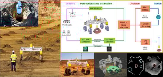
In this paper, we present the navigation and LiDAR-based perception framework for a blasthole seeking and dipping robot. Our contributions include a proximity-based adaptive navigation framework that dynamically switches between coarse GPS guidance and accurate target-seeking control. Our perception pipeline offers long-range 3D object detection, continuous tracking, and accurate in situ sensor insertion while compensating for variable cone geometries and noisy measurements during travel. The proposed framework fully leverages domain knowledge from surface mining processes, avoiding costly map construction or data collection while enabling unsophisticated configuration and straightforward deployment.

Our paper is structured as follows. We first present an overview of our inspection robot system in Section 2. Next, we present our navigation strategy in Section 3 and then, in Section 4, we show how to achieve cone detection and target tracking by auto-adjusting the perceptive parameters while the robot is in motion. In Section 5, we first describe the method for generating well-segmented binary images, where the cone face is fully whitened and the hole is represented in black; then, we present our two-stage coarse-to-fine detection process, which achieves excellent detection accuracy by leveraging smart region extraction, optimal circle fitting, and non-maximum suppression. In the experimental Section 6, we present various test results.

2. System Overview

DIPPeR’s main task is to visit and inspect each blast hole in a mine site inspection mission. As illustrated in Figure 2, the robot is an autonomous ground vehicle equipped with GPS, IMU, and wheel encoders for navigation, as well as two ouster LiDARs for perception. The sensing and perception layers of the robot system consists of the following components: sensors, perception and state estimation, mission manager, motion planner, base controller, and dipping actuator.

Figure 2. Overview of the core system modules and control flow.

The GPS system continuously outputs robot poses in the global UTM coordinates. The localisation module outputs robot poses in the local coordinate frame (“Odom”, origin at start of mission); this is estimated using the proprioceptive sensors. Robot poses from both coordinate frames are fed to the decision-making module—the mission manager. The perception module is another continuously running sub-system, reporting detected cones and hole positions to the manager whenever they are available. The mission manager maintains a state machine, which continuously compares DIPPeR’s position in all coordinate frames, against either the designated waypoint GPS positions or detected target positions. Two possible actions are issued by the manager: navigate to the target or dip the hole.

Depending on the distance between the robot and the cone, as well as the cone’s height, the perception module auto-adjusts its target detection settings. This ensures consistent tracking of the target hole as the robot moves towards it.

3. Navigation Strategy

Our mission controller is a type of cyclic state machine, as depicted in Figure 3b. Our proximity-based adaptive navigation strategy is the backbone of this state machine, where each state follows its own coordinate frame and localisation method and is completely decoupled from the others.

Figure 3. The navigation system switches between three different coordinate frames over the course of a seek hole cycle: (i) it navigates to the GPS point in the UTM frame to a coarse accuracy; (ii) after detecting the cone, plans motion to the target in the Odom frame; (iii) after detecting the hole, performs fine-servoing in the Body frame; (iv) after successful alignment, dips the hole.

3.1. Decoupled Localisation

As shown in Figure 3a, there are three coordinate conventions used in this navigation system, namely the universal transverse mercator (UTM) reference frame; the local Odom frame, in which the origin is the inspection start position; and the robot body frame. Both the UTM and Odom frame follow the Easting-Northing-Up (ENU) convention, and the robot body frame follows a Forward-Left-Up (FLU) convention. We use the symbol ${}^{\mathrm{F}}\mathbf{T}$ to denote the target position in a reference frame $\mathrm{F}$ in superscript font on the left of $\mathbf{T}$.

Each hole to be inspected has a GPS position ${}^{\mathrm{U}}\mathbf{T}$ in the UTM frame pre-recorded by the driller. This value has a metre-level error. We define a circular search region centred at the designated point, with a radius of 4 m—sufficient to account for GPS positioning errors in the absence of RTK correction. Any cone detected in this region is considered a potential candidate containing the actual hole. In the event of multiple detections, the cone with the smallest line-of-sight (LOS) angle to the robot heading is chosen as the matching hole for inspection.

When the robot initially detects a target hole in its body frame, denoted as ${}^{\mathrm{B}}\mathbf{T}$, the target is locked via the instantaneous body-to-global transformation (regardless of the correctness of this transformation) to position ${}^{\mathrm{U}}\mathbf{T}$ in the “UTM” frame. Similarly, via the instantaneous body-to-world transformation, the target is locked to ${}^{\mathrm{O}}\mathbf{T}$ in the “Odom” frame.

As DIPPeR moves around, and in the absence of RTK correction, its GPS measured position ${}^{\mathrm{U}}\mathbf{D}\left(t\right)$ in the UTM frame exhibits frequent jumps due to factors such as atmospheric disturbances and satellite orbital variances. Its distance to a detected target in this frame ${}^{\mathrm{U}}\mathit{l}=|{}^{\mathrm{U}}\mathbf{D}\left(t\right)-{}^{\mathrm{U}}\mathbf{T}|$ also exhibits corresponding shifts in value. UTM position-guided navigation works well for long-distance travel, where the accuracy requirement is low. However, for close-distance navigation, a controller that relies on the erroneous UTM distance would lead to random steering behaviour, to losing sight of the target, and eventually to navigation failure.

On the other hand, the robot’s position in the Odom frame ${}^{\mathrm{O}}\mathbf{D}\left(t\right)$ evolves smoothly as it is computed from the continuous integration of odometer measurements; this is an accurate estimate of the robot’s pose over a short duration. The “Odom” frame target distance ${}^{\mathrm{O}}\mathit{l}=|{}^{\mathrm{O}}\mathbf{D}\left(t\right)-{}^{\mathrm{O}}\mathbf{T}|$ exhibits a steadily decreasing trend to settlement. A controller that relies on this Odom distance should lead to eventual target contact. This is the motivation behind our decoupled localisation scheme. No attempt is made at fusing the GPS measurements with local odometry during the entire inspection mission.

3.2. Control Paradigm

Upon mission initiation, the robot navigates towards the GPS position of the first blast hole in the sequence, relying on its on-board GNSS antenna for position feedback, and navigating in the UTM frame.

Once within ∼4 m of the blast hole cone, DIPPeR can reliably detect the target, thus triggering the fine motion planning stage. The robot plans its trajectory, with the detection result as the goal, tracking the target continuously as the distance reduces. Localisation is performed in the local “Odom” frame to produce smooth pose estimates and avoid any discontinuities due to GPS drift or error. Furthermore, the robot may re-align its heading to the cone centre during this stage if the LOS exceeds a certain threshold.

Once within one metre of the target, the robot transitions into the fine positioning (visual servoing) stage. At each step, a velocity command is issued in the robot body frame based on the current relative target pose. Servoing on the detected hole centre continues until the sonde is precisely aligned. This process is repeated for each of the holes in the sequence, negotiating a boustrophedon coverage pattern [29] over the grid of blast holes.

The proposed strategy fully utilises the known structure of the blast bench during planning and execution, eliminating costly mapping operations and mitigating the impacts of GPS localisation discontinuity. More details on the implementation specifics of the robot control are presented in Section 6.1.2.

4. Target Detection and Tracking

For successful hole inspection, DIPPeR must autonomously detect not only the holes but also the cones that obscure them, and track these features during approach to enable precise probe insertion. As shown in Figure 4, cones and holes are detected by processing point clouds from the two on-board LiDARs and projected images generated from these point clouds. When positioned to face a cone at a certain distance, the robot relies on its forward-facing wide FOV LiDAR to detect the cone, as it is the only large above-ground object within the prescribed search region. Initially, from a far distance, the cone occludes the hole when viewed from ground level. As the robot approaches the target, the high-resolution downward-looking LiDAR gradually reveals the hole’s position. Assuming both the cone and hole have symmetrical shapes, moving towards the object centre ensures continuous detection during subsequent servoing operations. This serves as the basis for successful 3D object tracking. To maintain accurate hole detection in the image domain, the tracking system continuously adjusts the projection and detection parameters based on the hole’s distance from the robot.

Figure 4. Detection and tracking process.

4.1. Ground Tilt Correction

The first step in LiDAR processing concerns transforming the point clouds to a ground-aligned coordinate frame. This allows simple blast cone point extraction by thresholding using point heights. In instances where the robot is straddling a large cone and is tilted relative to the ground, as shown in Figure 5, the on-board orientation sensor can be used to apply a correction. To this end, we make use of the geo-referenced orientation measurements provided by the on-board 9-DOF IMU.

Figure 5. Robot base tilt correction. Correcting robot tilt is equivalent to rotating the base plane about vector $\widehat{\mathbf{v}}$ by angle $\theta$ to re-align the vehicle’s x–y axis with their projections on the ground. Note for (a), ©Rio Tinto 2025, All Rights Reserved. Three-dimensional surface model generated using DroneDeploy, Inc. software. Visualised using Gazebo [11.0/Open-Robotics].

By analysing the relative rotation between the ground plane normal ${\widehat{\mathbf{n}}}_G$ and the robot base normal ${\widehat{\mathbf{n}}}_R$, we can correct for the roll-pitch tilt experienced by the robot.

We make use of the robot’s shadow (approximately) on the ground to define a coordinate frame level on the ground at the robot’s position. LiDAR point clouds should be transformed to this shadow’s frame for further processing. For this, first we determine the rotation in the geo-referenced frame that aligns the robot base to its shadow.

$$\begin{array}{cc}\hfill \mathrm{Given}& \mathrm{the}\mathrm{true}\mathrm{ground}\mathrm{normal}\hfill \\ \hfill {\widehat{\mathbf{n}}}_{\mathrm{G}}& ={[x_{\mathrm{G}},y_{\mathrm{G}},z_{\mathrm{G}}]}^{⊺}\approx [0,0,1],\hfill \\ \hfill \mathrm{and}& \mathrm{the}\mathrm{robot}’\mathrm{s}\mathrm{orientation}\mathrm{in}\mathrm{the}\mathrm{geo}‐\mathrm{frame}\hfill \\ \hfill {\mathbf{R}}_{\mathrm{geo}}& =[{\mathbf{r}}_x,{\mathbf{r}}_y,{\mathbf{r}}_z]:\hfill \\ \hfill \mathrm{so}& \mathrm{robot}\mathrm{base}\mathrm{normal}{\widehat{\mathbf{n}}}_{\mathrm{R}}\mathrm{in}\mathrm{the}\mathrm{geo}‐\mathrm{frame}\mathrm{is}\mathrm{as}\mathrm{follows}:\hfill \\ \hfill {\widehat{\mathbf{n}}}_{\mathrm{R}}& ={\mathbf{r}}_z={[x_{\mathrm{R}},y_{\mathrm{R}},z_{\mathrm{R}}]}^{⊺}.\hfill \end{array}$$

(1)

We derive the rotation matrix (in the geo-frame) to align the robot’s base plane to its shadow on the ground. We can achieve this using the cross-product and the exponential map [30].

$$\begin{gathered} \begin{array}{c}\hfill {\mathbf{R}}_{\mathrm{align}}=\mathrm{Exp}\left(\widehat{\mathbf{v}}\theta \right),\end{array} \\ {\widehat{\mathbf{n}}}_{\mathrm{G}}={\mathrm{R}}_{\mathrm{align}}{\widehat{\mathbf{n}}}_{\mathrm{R}}; \\ \mathrm{where}\widehat{\mathbf{v}}={\displaystyle \frac{{\widehat{\mathbf{n}}}_{\mathrm{R}}\times {\widehat{\mathbf{n}}}_{\mathrm{G}}}{\parallel {\widehat{\mathbf{n}}}_{\mathrm{R}}\times {\widehat{\mathbf{n}}}_{\mathrm{G}}\parallel }},\theta =\mathrm{atan}2(\parallel {\widehat{\mathbf{n}}}_{\mathrm{R}}\times {\widehat{\mathbf{n}}}_{\mathrm{G}}\parallel ,{\widehat{\mathbf{n}}}_{\mathrm{R}}·{\widehat{\mathbf{n}}}_{\mathrm{G}}). \end{gathered}$$

(2)

Now, we can determine the orientation of the robot’s shadow in the absolute geo-frame.

$${\mathbf{R}}_{\mathrm{shadow}}={\mathbf{R}}_{\mathrm{align}}{\mathbf{R}}_{\mathrm{geo}}$$

The axis of rotation in the shadow’s frame is

$${\widehat{\mathbf{v}}}^{\mathrm{S}}={\mathbf{R}}_{\mathrm{shadow}}^{⊺}\widehat{\mathbf{v}}$$

Therefore, the robot orientation in its shadow frame is

$${\mathbf{R}}_{\mathrm{R}}^{\mathrm{S}}=\mathrm{Exp}(-{\widehat{\mathbf{v}}}^{\mathrm{S}}\theta )$$

(3)

This rotation should be used to transform LiDAR points from the robot frame to the ground-aligned frame.

4.2. Cone Detection

Against the flat ground of the bench, cones can be detected by height thresholding. We use long-range low-resolution LiDAR for long-distance cone detection. But once the robot reaches a 3 m distance, DIPPeR switches to short-range, high-resolution LiDAR for cone and hole detection. Furthermore, a series of box filters are applied to eliminate LiDAR points reflected off the robot’s body parts, including the four wheels and the chassis box.

Using the assumption that the bench is free from foreign objects, we classify any large point cluster contained within the 6 m corridor in front of the robot above a certain size as the cone object, avoiding computationally expensive 3D shape analysis. After removing noise points floating above the cone surface or inside the hole cavity, the filtered cloud appears as a clean surface.

The cone centre should be computed here as it is used in subsequent depth image projection. To avoid biassing due to the uneven distribution of LiDAR points, we use a 2D voxel grid to group the cone points, then compute the weighted average of the non-empty voxels using the voxel height as the weight to obtain a fair centroid estimate.

Due to frequent geological sampling, the cone surface may contain shallow pits around its edge (Figures 1a and 11). These pits can be erroneously detected as the blastholes causing the robot to go astray. To eliminate these ‘phantom’ holes, we fit a Convex Hull to retain LiDAR points from its shallow base that lie within the cone circumference. This ensures that the 2D-projected cone face appears consistent and unmarred by pitting. Further phantom hole treatment will be applied in the 2D image domain in Section 5.2.3.

4.3. Virtual Image Formation

Hole detection takes place in the 2D image domain. These 2D images are generated by projecting the cone cloud through a virtual camera at different positions above the cone. According to the projective geometry principle [22], the conversion of 3D points $\mathbf{P}=(x,y,z)$ to 2D image pixels $\mathbf{p}=(u,v)$ and the converse image-to-3D unprojection can be summarised as follows:

$$\underset{3\mathrm{D}‐\mathrm{to}‐2\mathrm{D}}{\underbrace{\mathbf{p}=\left[\begin{array}{c}u\\ v\\ 1\end{array}\right]={\displaystyle \frac{1}{z}}K\mathbf{P}={\displaystyle \frac{1}{z}}\left[\begin{array}{ccc}{f}_x& 0& c_x\\ 0& f_y& c_y\\ 0& 0& 1\end{array}\right]\left[\begin{array}{c}x\\ y\\ z\end{array}\right]}},\underset{2\mathrm{D}‐\mathrm{to}‐3\mathrm{D}}{\underbrace{\mathbf{P}=\left[\begin{array}{c}x\\ y\\ z\end{array}\right]=z{K}^{-1}\mathbf{p}=z\left[\begin{array}{ccc}{\displaystyle \frac{1}{f_x}}& 0& -{\displaystyle \frac{c_x}{f_x}}\\ 0& {\displaystyle \frac{1}{f_y}}& -{\displaystyle \frac{c_y}{f_y}}\\ 0& 0& 1\end{array}\right]\left[\begin{array}{c}u\\ v\\ 1\end{array}\right]}}$$

(4)

where $f_{x,y}$ and $c_{x,y}$ are the focal lengths and camera centre in the horizontal and vertical directions, respectively. Combined with image resolution $H\times W$, they are commonly referred to as camera FOV and are maintained as the virtual camera calibration settings in the rest of the paper for simplicity.

$${\mathrm{FOV}}_x=2arctan\left({\displaystyle \frac{W}{2f_x}}\right),{\mathrm{FOV}}_y=2arctan\left({\displaystyle \frac{H}{2f_y}}\right)$$

Knowledge of the camera’s FOV allows for easy conversion between the 2D image domain and 3D points. We maintain two copies for each projected virtual image; one encodes the point depth for each pixel, while the other is a binary image in which any non-zero depth is assigned the maximum grey-scale and the empty depth is labelled zero. In all filtering and detection steps, the binary image is used for ease of segmentation. Once the optimal 2D hole centre is estimated, we retrieve the depth from the corresponding pixel in the encoded depth map and unproject it to the 3D world using Equation (4). Then, a further transformation would produce the robocentric frame position for subsequent approach actions.

The FOV settings can also affect the following aspects of the virtual image: cone face coverage, pixel spacing, and hole object size. This is illustrated in Figure 6. Furthermore, non-central projection causes the hole to appear more elliptical. To address this, the virtual camera settings should be auto-adjusted at various distances during target tracking.

Figure 6. At various distances to the robot, by adjusting the virtual camera’s height and Field-of-View $\mathrm{FOV}$, the hole (shown as red-coloured region labels) is consistently located in the centre of the virtual images with similar sizes. The large hole opening of the high cone is due to hole’s funnel shape and beam occlusion. Projection setting include “Distance/Height/FoV”.

4.4. Tracking with Distance-Dependent Image Projection

Due to beam divergence, LiDAR coverage on the cone face can vary significantly at different distances. To further complicate the situation, the holes are not perfectly cylindrical but have a funnel-shaped opening which narrows down to a cylinder about 30 cm below the ground and extends to a depth of several metres. These factors can cause significant variations in hole imprint in 2D images. To solve this problem, we apply a three-way proximity-based camera setting adjustment, which adaptively configures the virtual camera height, FOV, and image processing filters to match the changing data resolution. We define a look-up table (Figure 7) to model the variation in optimal camera settings as a function of cone distance.

Figure 7. A cone’s distance and height has an effect on the virtual camera settings and the size of the smoothing filter. (a) Camera heights/filter size increase as the cone distance increases. (b) Plot of scaling Equation (5) that maps the cone height’s to the camera height.

4.4.1. Point Sparsity

Point sparsity stems from the fact that the density of LiDAR points covering the cone varies with distance. Further-away cones with larger beam spacings lead to large inter-pixel voids, while closer cones reflect a denser beam pattern and hence a reduced porosity (see Figure 6a–c for an illustration). For ease of image segmentation, a smooth cone face object is desired, where all sparsity-induced voids are filled. To achieve this, we apply a number of morphological and smoothing filters (Section 5), the configurations of which are defined in the lookup table in Figure 7, where the kernel size increases as the cone distance increases.

4.4.2. Cone Face Coverage

To successfully locate the hole, as much of the cone face should be exposed as possible, especially at far distances. This is achieved by increasing the camera’s FOV such that more points are encompassed within the image frame.

4.4.3. Hole Size

The cone distance affects the extent of hole occlusion—the hole void is more likely to be missed when the robot is far away. This, together with the hole’s funnel shape can cause the hole imprint to appear larger at long distances, narrowing down towards a circle as the robot gets closer. As shown in Figure 6, increasing the camera height for further-away cones can mitigate this problem.

4.4.4. Cone Height

At the same distance, high cones can cause further hole occlusion, resulting in more pronounced variation in hole footprint (see Figure 7a for an illustration). We apply further camera height adjustment, shown in Equation (5), to ameliorate this effect:

$$z_{cam}^s=z_{cam}\times \max (1-{\displaystyle \frac{0.9}{1+\exp (6.25h-2.88)}},0.6),$$

(5)

where the parameters have been chosen to produce the profile in Figure 7b. This gives large camera depth to high cones, ensuring sufficient hole inclusion in the projected image.

Both the lookup table and the scaling function are easy to generate and can be configured based on LiDAR FoV and beam number rating, and by online observations of intermediate hole detection results, as shown in Figure 8.

Figure 8. Single-shot hole detection. See the enumerated list in Section 5 for explanation of subfigures.

5. Hole Detection

Due to the data availability concerns outlined in Section 1, we elected to adopt a classic detection approach with hand-crafted feature extraction and probability analysis for optimal candidate selection. This approach builds on our previous work [31] on a two-stage coarse-to-fine detection pipeline. The projection point for the virtual camera across all stages is determined by the cone centre identified by coarse stage detection. The fine detection stage is then only activated when the robot is in close proximity to the target. The entire detection pipeline is shown in Figure 8; a description of the steps is listed below.

1.

Apply coarse projection (Figure 8a) using cone centroid as the projection point—this usually does not coincide with the hole centre and gives a distorted view of the circle, as shown in Figure 8b.

2.

Apply morphological operators and Gaussian blur filters to fill up spacings from sparse points. After binary thresholding, a well-rendered whole-cone object appears and is segmented from the hole (see Figure 8c).

3.

Identify the hole object using simple moment analysis (see Figure 8d).

4.

Apply fine-stage projection using the blob centre as the projection point; the hole object is at the centre of the new image and is very circular (see Figure 8e).

5.

Apply similar morphological operations to form a connected cone object, then extract features to identify circular regions (see Figure 8f).

6.

With optimal circle fitting and non-maximum-suppression, we identify the best circle (in red) in Figure 8g, and mark detection results in original virtual image Figure 8h.

7.

Compute the hole’s 3D position by first back-projecting the 2D centre on the stored depth map value using Equation (4), then another transform to determine the robot-centred coordinates.

5.1. Coarse Detection

In this stage, standard contour methods are applied for hole detection. Since the cone and hole objects have fairly consistent sizes, simple thresholding can yield good detection results. Of all extracted contours, the largest one is usually the cone, shown in Figure 8d as a golden bounding box. If a void is found inside the detected cone, it is classified as the hole object if it is both of sufficient size and close to the image centre. A rough position of hole can thus be obtained after 2D–3D back-projection.

5.2. Fine Detection

To precisely determine the position and dimension of a hole, we project the cone point cloud one more time, with the virtual camera right above the detected blob centre. This ensures that the hole appears as a highly circular object in this second virtual image, avoiding any perspective effect.

We now present our optimal hole selection scheme, which is an extension of the optimal circle fitting algorithm in [31], with the addition of a non-maximum-suppression method.

5.2.1. FRST Feature and ROI Extraction

A Sobel filter is applied to the output of the morphological operation and a gradient image is produced, showing a virtual image with clear edges. We use hand-crafted Fast Radial Symmetrical Transform (FRST) [32] features to detect circular regions. These features behave like a 2D histogram; high counts indicate possible locations of the circle centre. The reader is advised to refer to Appendix A for further details. Pixels within an acceptable neighbourhood of the feature centre are referred to as Regions of Interest (ROI); circles can be identified from the extracted ROIs. Figure 9a shows an illustration of this process, where FRST feature points are blue blobs and extracted ROIs are red pixels. For the sake of completeness, we present the whole procedure.

Figure 9. FRST + ROI + RANSAC + Taubin.

5.2.2. RANSAC and Circle Fitting

Given a set of points that form a circle, we opt to use Taubin’s Least Squares Fitting algorithm [33] to find the optimal circle. For the sake of completeness, we list the problem statement here.

Let us denote $\mathbb{R}$ as the set of ROI in a given image I. Then, denote R as the set of valid pixels $R=\left\{{\mathbf{p}}_i=(u_i,v_i)\right\}$ with size $\left|R\right|$ from one FRST-generated ROI and let $\mathbf{\Theta }=(\mathbf{c},r)$ denote the circle fitted to the ROI with centre $\mathbf{c}=(a,b)$ and radius $r_i$. In order to derive a fitting algorithm agnostic to hole sizes, we focus on an optimal unit circle problem, and express each ROI point ${\mathbf{p}}_i$ as a normalised directional vector $(cos\left({\varphi }_i\right),sin{\left(\varphi \right)}_i)$ pointing to the circle centre with incidence angle ${\varphi }_i$:

$$\begin{array}{cc}\hfill cos{\varphi }_i& ={\displaystyle \frac{u_i+{\delta }_i-a}{r}}={\displaystyle \frac{u_i-a}{r}}+{\tilde{\delta }}_i,{\tilde{\delta }}_i={\displaystyle \frac{{\delta }_i}{r}}\in \mathcal{N}(0,\sigma )\hfill \\ \hfill sin{\varphi }_i& ={\displaystyle \frac{v_i+{ϵ}_i-b}{r}}={\displaystyle \frac{v_i-b}{r}}+{\widetilde{ϵ}}_i,{\widetilde{ϵ}}_i={\displaystyle \frac{{ϵ}_i}{r}}\in \mathcal{N}(0,\sigma ).\hfill \end{array}$$

(6)

where $\delta$ and $ϵ$ denote the errors in the u and v directions, respectively, and are converted to normalised form $\tilde{\delta }$ and $\widetilde{ϵ}$ in order to follow an independent and identically distributed (IID) normal distribution around each point along the unit circle’s circumference, where the distribution’s standard deviation is standardised to $\sigma$.

In an effort to minimise sum of the normalised errors and avoid non-linearity-related convergence issues, Taubin presented the following formulation in [34]:

$$\begin{array}{cc}\hfill \mathrm{Solve}\mathbf{\Theta }& =\mathrm{argmin}{\mathcal{F}}_{\mathrm{T}}(\mathbf{\Theta })\hfill \\ \hfill \mathrm{where}{\mathcal{F}}_{\mathrm{T}}& ={\displaystyle \frac{\mathrm{\Sigma }{[{(u_i-a)}^2+{(v_i-b)}^2-r^2]}^2}{4n^{-1}\mathrm{\Sigma }[{(u_i-a)}^2+{(v_i-b)}^2]}},n=\left|\mathbb{R}\right|.\hfill \end{array}$$

(7)

A change in parameters transforms (7) into a constrained linear least squares problem:

$$\begin{array}{cc}\hfill & {\mathcal{F}}_l=\sum _{i=1}^n{(A{w}_i+B{u}_i+C{v}_i+D)}^2,\hfill \\ \hfill \mathrm{subject}\mathrm{to}& 4A^2{M}_w+4AB{M}_u+4AC{M}_v+B^{2}n+C^{2}n=1,\hfill \\ \hfill \mathrm{where}& w_i=u_i^2+v_i^2,B=-2aA,C=-2bA,D=a^2+b^2-r^2\hfill \\ \hfill \mathrm{and}& M_u=\sum _{i=1}^n{u}_i,M_v=\sum _{i=1}^n{v}_i,M_w=\sum _{i=1}^n{w}_i.\hfill \end{array}$$

(8)

This circle fitting problem can now be further transformed into an Eigen decomposition-based approach which is completely linear and has an analytical solution. The details are given in Appendix B. This fast solution is amenable to simple deployment. We did not install GPU hardware on DIPPeR; all computations were achieved on a multicore computer. Taubin’s algorithm has an important property [33]—the solutions are independent of the choice of coordinate frame, i.e., they are invariant under translations and rotations. This fully respects the circular hole’s radial symmetry, without coercing for a meaningless orientation. The residuals’ IID distribution around the smooth circumference of the circle contrasts with other non-ideal methods, such as in [11], where a circle is treated as a polygon and piece-wise linear HOG features are extracted around the hole circumference then coerced to describe a circular geometry via non-linear SVM regression. Such methods require a large amount of data augmentation in order to cater for all orientations subject to finite angular resolution.

Since not all points in the ROI are part of the circle, we separate the valid pixels and outliers in a RANSAC [35] framework based on Taubin’s algorithm. Starting with a seed of trial samples, a small well-fitted circle is found first; then, this circle is grown by adding more points that satisfy the current constraint. This process is repeated until circle growth converges or the max iteration number is reached. Since Taubin’s algorithm is a type of convex optimisation, each iteration is guaranteed to converge to the optimal fit. This ensures that the RANSAC process leads to the largest optimal circle in an ROI. The result of RANSAC for each ROI is illustrated in Figure 9b–d. Since RANSAC is a very expensive operation, we set a cap of 100 on the number of retries in the candidate RANSAC process to achieve a balance between fitting accuracy and visual servoing delay.

Our method provides highly accurate detection results, yet works fast in real time, without using an expensive data-learning-based process or expansive hardware. It is therefore highly suitable for in situ robot inspection applications.

5.2.3. Non-Maximum Suppression

The previous steps can produce multiple candidate circles (see Figure 1f, Figure 8g and Figure 9b). This is exacerbated when phantom holes appear in non-vertical LiDAR scans, as Convex Hull cannot completely eliminate them. We provide a non-maximum suppression (NMS) scheme to select the best candidate, taking into consideration the following factors: the FRST feature strength, the candidate’s distance to image centre, and the circular goodness of fit.

Before presenting any rigorous analysis, we first define some simple switching logic to discard invalid candidates. This is analogous to the Relu operation in a NeuralNet system:

• The circle radius is in a prescribed range;
• The circularity score (Equation (13)) is above a threshold;
• More than 70% of the region is black;
• The centrality score (Equation (12)) is above a threshold;
• The FRST feature score (Equation (11)) is above a threshold.

Continuing from the problem stated in Section 5.2.2, we re-use the notations here, where $R_i$ denotes the set of valid pixels $R_i=\left\{{\mathbf{p}}_i\right\}$ with size $\left|R_i\right|$ from the i’th FRST generated ROI and ${\mathbf{\Theta }}_i=({\mathbf{c}}_i,r_i)$ denotes the circle fitted to the ROI with centre ${\mathbf{c}}_i$ and radius $r_i$. To find the best circle ${\Theta }^{\ast }$, we first define the occurrence probability $P\left({\Theta }_i\right|I)$ of the i’s candidate circle as

$$\begin{array}{cc}\hfill P\left({\mathbf{\Theta }}_i\right|I)& ={\mathrm{\Sigma }}_{r}P\left(R_r\right|I)P\left({\mathbf{\Theta }}_i\right|R_r)\leftarrow \mathrm{Marginalise}\hfill \\ \hfill & =P\left(R_i\right|I)P\left({\mathbf{\Theta }}_i\right|R_i)\leftarrow \mathrm{Simplify}\hfill \\ \hfill & \propto P\left(R_i\right|I)P\left({\mathbf{\Theta }}_i\right)P\left(R_i\right|{\mathbf{\Theta }}_i)\leftarrow \mathrm{Bayes}\mathrm{rule}\hfill \\ \hfill & \propto P\left(R_i\right|I)P\left({\mathbf{\Theta }}_i\right)\prod _{{\mathbf{p}}_j\in R_i}P\left({\mathbf{p}}_j\right|{\mathbf{\Theta }}_i)\leftarrow \mathrm{Likelihood}\hfill \end{array}$$

This best circle ${\mathbf{\Theta }}^{\ast }$ should correspond to the highest probability of occurrence or the maximum a posteriori estimate. This allows us to define the confidence score ${\mathcal{S}}_{conf}\left({\mathbf{\Theta }}_i\right)$ on candidate ${\mathbf{\Theta }}_i$ as a weighted sum of the ROI quality score ${\mathcal{S}}_F\left(R_i\right)$, regularisation score ${\mathcal{S}}_{reg}\left({\mathbf{\Theta }}_i\right)$, and circularity fit score ${\mathcal{S}}_{circle}\left({\mathbf{\Theta }}_i\right)$.

$${\mathcal{S}}_{conf}\left({\mathbf{\Theta }}_i\right)={\alpha }_1{\mathcal{S}}_F\left(R_i\right)+{\alpha }_2{\mathcal{S}}_{reg}\left({\mathbf{\Theta }}_i\right)+{\mathcal{S}}_{circle}\left({\mathbf{\Theta }}_i\right).$$

(9)

The best circle is the one with highest confidence:

$${\mathbf{\Theta }}^{\ast }=\underset{i\in \left|\mathbb{R}\right|}{\mathrm{argmax}}{\mathcal{S}}_{conf}\left({\mathbf{\Theta }}_i\right)$$

(10)

The ROI quality is determined by the FRST feature quality; a high feature count $\left|F_i\right|$ strongly implies the existence of a circle.

$${\mathcal{S}}_F\left(R_i\right)={\displaystyle \frac{1}{1+3exp(3-0.1\left|F_i\right|)}}\in [0\sim 1]$$

(11)

Despite using the Convex Hull filtering operation described in Section 4.2, phantom holes can still appear in the cone face due to partial LiDAR scan occlusion at oblique angles. As bore holes are located at the blast cone centre, we add a regularisation term to penalise phantom holes that are further from the apparent cone centre:

$${\mathcal{S}}_{reg}\left({\mathbf{\Theta }}_i\right)={\displaystyle \frac{1.2}{1+50exp(0.05\parallel {\mathbf{d}}_i\parallel -5.5)}}\in [0\sim 1],$$

(12)

where ${\mathbf{d}}_i={\mathbf{c}}_i-{\mathbf{o}}_I$ is the distance vector from the circle centre to the image centre ${\mathbf{o}}_I$.

To evaluate how well the ROI points fit a circular hole, it is necessary to consider both residual errors and the ROI’s angular coverage on the full circle. We define a circular grid of B bins around the hole to sort points into the relevant bins from their angles of incidence. We compute each bin’s mean-squared-error $e_b$ and then map it to a bin probability score $H_b$. The circularity score is the sum of individual bin scores:

$${\mathcal{S}}_{circle}\left({\mathbf{\Theta }}_i\right)={\displaystyle \frac{1}{B}}\sum _{b=1}^B{H}_b\in [0\sim 1],$$

(13)

where bin score $H_b$ is a type of probability mapped from bin mean-squared error (MSE)

$$\begin{array}{cc}\hfill H_b=& \exp (-{\displaystyle \frac{1}{2}}{\displaystyle \frac{e_b}{{\sigma }^2}})\in [0\sim 1],\hfill \end{array}$$

(14)

and bin MSE $e_b$ accumulates all point errors in bin b

$$\begin{array}{cc}\hfill \forall j\in \left|R_i\right|,& {\mathbf{v}}_j={\displaystyle \frac{1}{r_i}}({\mathbf{p}}_j-{\mathbf{c}}_i),\hfill \\ & e_j=\parallel {1-\parallel {\mathbf{v}}_j\parallel \parallel }^2,b=\mathrm{Bin}\left(arctan\left({\mathbf{v}}_j\right)\right),\hfill \\ & {e_b}^{+}=\frac{n_b^{-}{e}_b^{-}+e_j}{{\hat{n}}_b^{-}+1},n_b^{+}=n_b^{-}+1.\hfill \end{array}$$

(15)

6. Experiments

We tested DIPPeR’s navigation and perception systems using both simulation and real-world data. For simulations, we build a simulated world in Gazebo with 3D terrain meshes from various sources. Similarly to in our previous work [31], we added hollow cylinders with prescribed diameters in the 3D mesh to resemble blast holes. For real-world tests, we performed extensive tests on the DIPPeR platform. These include numerous functional tests on the Sydney University Campus and two site trials at mine blast-sites in Australia and the USA. A demonstration video is available at https://www.youtube.com/watch?v=fRNbcBcaSqE (accessed on 16 November 2025).

6.1. DIPPeR Design

6.1.1. Hardware Configuration

The DIPPeR robot is a 3.8 m wide, 2.4 m long omnidirectional platform with 1.3 m of ground clearance, capable of in-place rotation. Weighing approximately 320 kg, it can achieve speeds of up to 1 m/s.

The platform is equipped with two LiDAR sensors: a 32-beam Ouster OS-1 [36] for situational awareness and cone detection, and a 128-beam Ouster OS-0 [37] for high-precision hole detection. The DIPPeR platform uses an Advanced Navigation Certus dual antenna GNSS/INS [38], capable of achieving ±1.2 m accuracy in absence of RTK. Certus also includes a 9-DOF IMU device, which uses high-precision, temperature-stabilised MEMS sensors to measure linear acceleration, angular velocity, and magnetic field strength. These are fused with the GNSS solution to provide roll, pitch, and heading accuracy of 0.1 degrees. It also serves as the GNSS-disciplined clock for our PTP and NTP network time synchronisation. The on-board computing platform is a 12-core Intel NUC 13 computer; it hosts all of DIPPeR’s software modules, which work seamlessly with the hardware enabling DIPPeR to conduct inspections continuously in real time.

6.1.2. Software Architecture

DIPPeR’s software modules include the Guidance, Navigation and Control (GNC) system and the perception system. Most of DIPPeR’s software was written in C++ and Linux scripts, using ROS Noetic [39], running on Ubuntu 20.04.

The GNC system makes use of the flexible and extensible move_base_flex (http://wiki.ros.org/move_base_flex) package, which, in addition to backwards compatibility with the standard Robot Operating System (ROS) move_base, also exposes a number of useful actions that allow for more complex interactions with motion controllers and planners. We specifically use A^∗ for global path planning and the Time Elastic Band (TEB) planner [40] for local trajectory planning. We additionally developed a ROS controller for omnidirectional swerve-steer platforms, such as DIPPeR, which executes twist commands from the navigation system while satisfying steering angle constraints.

The global and local path planners are invoked during the global and fine planning stages of the seek-hole cycle, operating in the UTM and Odom frames, respectively. The robot’s UTM coordinates are accessible directly from the Certus INS. We obtain an estimate of the robot local odometry by running an EKF [41] in local mode to fuse the wheel odometry and the IMU. Upon transition to the fine positioning stage, visual servoing is performed on the detected hole centre, transforming the position from the virtual camera frame to the robot body frame to determine the positional offset, and then driving the robot’s sonde axis towards that location. This process fully exploits the pseudo-omnidirectionality of the platform’s motion to precisely position the body of the robot for subsequent down-hole sensing.

We developed our proprietary decision-making and target detection system in C++. For 3D LiDAR processing, we made extensive use of the PCL library [42], and for 2D hole detection, we used both the OpenCV library [43] for basic image processing and the circle_fit library [44] for implementation of Taubin’s algorithm. The perception system is capable of processing three hole detections per second, which at the operating speed of the platform, is sufficient to perform real-time hole inspection.

6.2. Feature Tests

6.2.1. Detection Accuracy Analysis—In-Lab Tests

We performed in-lab hole detection accuracy tests for three different cone set-ups: a 0.15 m-radius hole with a 0.5 m cone height (labelled as “r = 0.15, H”), a 0.15 m-radius hole with 0.3 m height (labelled as “r = 0.15, L”), and a 0.25 m-radius hole with a 0.9 m cone height (labelled as “r = 0.25, H”). We positioned the hole centre at a discrete level of distances, then recorded the estimated hole distances and radii, the plot of which is given in Figure 10. We observed that the estimated hole distances mirrored the ground truth distances, with a close-to-unity trend line. The estimated radii also closely match each of the bespoke hole object. The general trend is as follows—the closer the hole is to the LiDAR sensor, the more accurate the measurement becomes. These results are supportive of the success of visual servoing.

Figure 10. Collection of estimated hole distances and radii at various static positions: (a) Static detection test set-up; (b) estimated hole distances versus GT; (c) estimated hole radius versus distance. The plot in (b) resembles a unit-gradient line, illustrating high accuracy in hole distance estimation. The estimated hole radii in (c) closely match the tested hole object size for each labelled case, especially at close distances to the robot.

6.2.2. Single-Cone Visual Servoing—In-Lab Tests

We performed numerous in-lab visual servoing tests (more than 100 tests). In this case, the robot was positioned about two metres in front of a cone on a flat ground, corresponding to the situation in the visual servoing stage in our state machine from Section 3.2. The robot performs step-by-step advancement to align its sonde with the hole by issuing velocity commands based on the fine hole detection results. At a hardware level, we spent a significant amount of time tuning the swerve controller of the DIPPeR robot to ensure smooth manoeuvring. We also carefully calibrated the mounting positions of the sonde and the LiDAR and added compensation terms in the software configuration to cater for the time delay between the detection process and the continuous robot movements. With all this effort, the robot was able to release its sonde close to the hole centre without scraping the cavity wall in almost 100% of cases. This success allowed us to proceed to navigation-perception mission tests.

6.2.3. Detection Robustness Analysis—On Real-World Data

The field trial site in western Australia contains numerous cones with pits formed during geological sampling, which are the primary cause of detecting phantom holes. We noticed that the majority of phantom holes are transient and occur at distances between 0.3 m and 0.8 m to the robot, which form the right oblique incidence angles that prevent the LiDAR beams from reaching the ground. The combined use of Convex Hull in 3D cone detection (Section 4.2) and centrality regularisation in Hole Non-Maximum-Suppression (Section 5.2.3) is tested for preventing phantom holes. Our scheme was found to be able to successfully filter out more than 90% of the phantom holes encountered over the travelled distance. We also observed that when the robot moves at its normal speed of 0.4 m/s, with detection running at 3Hz, true-positive detection dominates and the robot is able to steer fairly straight forward to pass by this stage. Then, at closer distances, our RANSAC-based optimal circle-fitting algorithm (Section 5.2.2) provided reliable guidance, leading to 100% dipping success. We present examples of our phantom hole rejection and optimal circle fitting in Figure 11; more can be found in the released demo video.

Figure 11. Examples phantom holes and NMS-enhanced detection results: cyan coloured holes are suppressed candidates, red holes are the chosen ones. Note for left column: ©Rio Tinto 2025, all rights reserved.

6.2.4. Cone Detection Result—Simulated Data

We conducted tests to determine the cone detection accuracy of the high-density LiDAR at various positions in a simulated world using 3D mesh data generated by Bentley™ software [45]. About 5% of the 721 detections failed; the results are presented in Figure 12a, where blue dots indicated locations of successful detection and red dots indicate failures. We also grouped failed detections into histogram bins based on their distances to the robot. The failure distance histogram and converted cumulative distribution function are shown in Figure 12b. In the plot, a high cone detection failure rate is observed to occur in the distance range of $[3\mathrm{m}\sim 6\mathrm{m}]$, whereas the failure rate becomes very low once the robot distance reduces to three metres. This allows us to set the activation distance for high-density LiDAR processing, as described in Section 4.4, to start at 3 m distance.

Figure 12. Statistical analysis on safe cone detection distance in the simulated world. Note for subfigure (a): ©Rio Tinto 2025, all rights reserved. Three-dimensional surface model generated using Bentley Systems, Inc. software. Visualised using Gazebo [11.0/Open-Robotics].

6.2.5. Approach Behaviour Analysis—Real-World Data

We also tested our auto-adjust perception feature in a physical-world test. In Figure 13, below the perception results, DIPPeR’s motion sequence as it gradually approaches the cone/hole target is shown. The detection results are shown for six different distances: 3.51 m, 3.09 m, 2.51 m, 0.87 m, 0.50 m, and 0.01 m. At 3.51 m distance, the robot sees a cone target from its sparse LiDAR and has just transitioned from seek-GPS-point mode. At 0.01 target distance, the robot has stopped visual servoing and is in the process of performing hole-dipping. The changes in cone face density and hole sizes match the expected behaviour.

Figure 13. Approaching behaviour at various target distances. Cyan coloured circles are suppressed hole candidates, red contours are the chosen hole. For all inset photos: ©Rio Tinto 2025, all rights reserved.

6.2.6. Mission Test—On Usyd Campus

We performed a navigation system and mission control test on Sydney University Campus. This test involves running an inspection mission on a blast pattern of five holes. We prepared bespoke inflatable cones to emulate the profile of an average blast-hole cone, each with a 40 cm hole in the centre. The cones were arranged in a two-column blast pattern on Usyd Campus, each purposefully positioned with a metre-level offset error to some marked GPS point. This is illustrated in Figure 14, below. DIPPeR was able to complete the entire seeking and dipping mission for every hole without manual intervention. For each hole, DIPPeR acted according to the state machine, by first seeking the pre-recorded GPS point up to a rough position, then switching to motion planning to target after detecting the target. At a close distance, it was able to servo to the hole to dip its sonde.

Figure 14. Mission Test at Usyd campus: (a). Five-hole blast pattern at Usyd campus; (b). Dipping on an inflatable cone.

On the same university campus, we also conducted experiments on other navigation strategies using the same mission set-up. This included a fused GPS–Odometry localisation strategy and Odometry-only localisation strategy, which are referred to as “Map” and “Odom” strategies, respectively, from now on. We use the same state machine as described in Section 3.2 for operation control, but issue motion plans in a coordinate frame that matches the navigation strategy. In the “Map” strategy mission test, we used ROS robot localisation [41] to form the fused UTM–Odometry “Map” frame and converted all test hole GPS positions into this frame before running a mission. We observed that the robot frequently went in the wrong direction, which can be explained by the noisy GPS reception at the university campus. For the “Odom” strategy mission test, we did not apply any sensor fusion, but instead periodically updated the transformation from current odometry to the UTM frame as the test proceeded. The conversion of the test hole’s GPS position to the “Odom” frame was delayed until immediately before the hole’s seek cycle started. We observed that the robot steered in the right direction initially, but gradually lost its way after a few dips. This problem became more apparent when the robot performed large rotation manoeuvrers in the middle of seeking. The results of the three navigation strategy tests are compared in Table 1, showing statistical counts on successful runs and the total number of dipped holes. Our navigation system significantly outperforms the other strategies.

Table 1. Comparison of navigation strategies.

Navigation Strategy	Ours	Map	Odom
Total missions attempted	15	7	5
Successful missions	15	0	0
Total holes dipped	60	1	2
Tracks after rotation	Y	N	N

6.3. Comparison to Learning-Based Method— Real-World Data

Despite not taking a learning-based approach in our work, we did explore the potential of training a detection network on the classifications generated by our classical detection pipeline. We auto-generated 916 pairs of images and marked hole regions—similar to the examples in Figure 6c–e—to train Yolo 11 [46] for hole segmentation. We used 711 pairs as the training set and 205 pairs for validation. The majority of the segmentation results match our expectation for coarse-stage projection. Yolo yields validation results of 0.98 F1 score at 0.58 detection confidence. A selection of validation results are shown in Figure 15.

Figure 15. Yolo segmentation [46] using our detection outputs for training.

We used the trained Yolo model to perform an inference test for four specific categories and compared the results with the detection outputs of our approach. The four categories of test cases are as follows: generic (well-represented samples at all distances to target), feature sensitivity (distant cones or perspective viewing), phantoms holes and centre accuracy (during visual servoing). The results of precision–recall analysis of both methods are given in Table 2; example detection outputs from each are also included.

Table 2. Comparison of our hole detection results (red labels) against Yolo detections (blue masks) for four data categories: (a) generic—fair distribution of hole images over all distances; (b) feature sensitivity—for far-away cones; (c) phantom holes before the robot arrives at the hole; (d) hole detection centrality, when the robot is right above the hole.

Test Category	Ours		Yolo
	Confusion Matrix	Example	Confusion Matrix	Example
(a) General 260 samples
(b) Feature sn’tvt 38 samples
(c) Phantom hole 109 samples
(d) Hole centrl’ty 92 samples

For the generic category (row 1), the two approaches have comparable success rates, indicating the potential of using the classical pipeline for self-supervised learning. For the distant cone scenario (row 2), Yolo with a high precision and recall, outperforms our method in identifying large holes due to its richer feature space. Our approach performs poorly as its hand-picked Gaussian filter reaches its kernel limit. However, in latter detection stages, our scheme outperforms Yolo in terms of phantom hole rejection (row 3) and hole centre accuracy (row 4), achieving high precision and recall owing to the incorporation of NMS- and RANSAC-based least squares circle fitting methods. The latter result can be explained as follows; CNN features, analogous to the HOG features, are best for data with an underlying grid-like or Euclidean structure where the extraction operation takes the form of shifting a filter in the grid space along the direction of its spanning axis [47]. The resultant feature maps have a polygonal shape with piece-wise linear edges. Circles, owing to their curved geometry, require a rotation-invariant detection algorithm. Overall, our classic approach is more practical for this application and does not require data collection or labelling. Moreover, it is easy to reconfigure when the hole size specification changes.

6.4. Long-Duration Mission Test—Simulation

We simulated our autonomous mission system in the Gazebo environment, shown in Figure 16. The terrain mesh model was generated by DroneDeploy™ [48]. We further edited the mesh to add hole cylinders and created mission plans for this world, including hole GPS positions for inspection. Our system can successfully complete a 58-hole mission test repetitively.

Figure 16. Extended mission test in Gazebo simulation. Left: simulated world, ©Rio Tinto 2025, all rights reserved. The 3D surface model was generated using DroneDeploy, Inc. software. Visualised using RViz[Noetic/Open-Robotics] and Gazebo [11.0/Open-Robotics]. Right: bottom 3D panel shows pre-recorded GPS points (magenta bars), mission trajectory (blue) and target search region (dark green patch); top 2D panel shows coarse detection result (masked blob), FRST feature (blue blob), fine detection result (red circle).

6.5. Site Trials

We conducted site trial runs of DIPPeR in western Australia in 2023 and Utah in 2024 at two different mines that produce different minerals with different cone geometries and hole diameters. The WA trial was conducted during the hotter months, where temperatures inside the robot’s sealed metal enclosures can reach up to 100 °C. The Utah trial was conducted in sub-zero conditions during snowfall, with the ground covered in ice and snow.

When trial runs are conducted during active production, the experiments must be brief because there is limited time available between drilling and charging for blasting, sometimes only few hours. As a result, access to any given blast site is extremely time-limited. During these trials, the on-board sensing and perception system was operated in real time, while all sensor data was recorded for offline analysis and algorithm refinement. This approach enabled us to use real-world data to validate the improvements made between trials, helping us prepare more effectively for each subsequent run.

For the WA trial run (Figure 17), the cones were well formed. A total of 95 holes were successfully detected, and the sensor-to-hole alignment was perfect (successful on nearly 100% of attempts) for the 38 holes dipped. However, in the Utah trial run, the shape of the drill waste resembled a bowl rather than a cone. The wide circumference and shallow hole centre of the waste caused significant occlusion, preventing the LiDAR beams from fully reaching the cone centre and leading to the presence of large hollow patches in random places over the cone face in the projected 2D images. Detection and alignment were successful in more than half of the attempts in the 70 inspected holes. To address occlusion-related detection failures, we may need to increase the mounting height of the high-definition LiDAR to improve the coverage of the cone interior. This can be verified in future tests.

Figure 17. Long-duration test in WA, Australia. Left: aerial image of DIPPeR inspecting a blast site, ©Rio Tinto 2025, all rights reserved. Inspection visualised using RViz[Noetic/Open-Robotics]. Right: bottom 3D panel shows mission trajectory (red), cone points (green); top 2D panel shows suppressed candidates (cyan), FRST features (blue dots), coarse detection result (masked blob) and fine detection result (red circle).

The success rates achieved in both trial runs—particularly in the former environment—are promising and demonstrate the effectiveness of the proposed concept for efficient and informative hole inspection.

7. Conclusions

In this paper, we presented a practical perception and navigation solution for the industrial application of autonomous blast hole dipping, implemented on the DIPPeR mine site inspection robot. Effective hole inspection was demonstrated without requiring mapping, heavy-duty detection algorithms, or extensive data collection, labelling, and training. All software computations took place on a multicore computer without requiring dedicated GPU hardware. An adaptive proximity-based navigation strategy handles the transition from imprecise GPS positioning to relative localisation to the blast holes using the proposed classic vision-based detection algorithm for proximity navigation, tracking, and servoing. For an early proof of concept, we constructed a Gazebo simulation world with a third-party generated 3D mesh model and manually inserted hollow cylinders with set dimensions for hole detection testing. This allowed an evaluation of the proposed target-tracking method to be conducted through tuning virtual camera projection parameters at different target distances. The simulation results verify the feasibility of our navigation and perception design choice. The subsequent lab tests and on-campus tests consistently demonstrated that our framework can seek targets reliably in continuous inspection missions and achieve precise alignment of the sensor above the bore holes. The early field trial success in western Australia further illustrates the strong potential of robotization of blast hole inspection with a practical approach, which would lead to significant cost savings and improved working conditions for personnel.

For sites with irregular cone geometries, more investigation is needed. The irregular, unpredictable, and non-repetitive cone shapes make it challenging to choose detection parameters that perform well across all scenarios. As the robot inspects new blast hole patterns, the detection parameters can be progressively optimised based on the most frequently observed cone shapes. Consequently, the detection success rate is expected to improve as more sites with different blast hole patterns are visited. Moreover, the growing dataset of cone shapes will eventually enable the training of a neural network model, further enhancing detection robustness and generalisation.

References

- Noopur, J. An Overview of Drilling and Blasting in Mining. AZoMining 2025. Available online: https://www.azomining.com/Article.aspx?ArticleID=1848 (accessed on 16 November 2025).
- Kokkinis, A.; Frantzis, T.; Skordis, K.; Nikolakopoulos, G.; Koustoumpardis, P. Review of Automated Operations in Drilling and Mining. Machines 2024, 12, 845. [Google Scholar] [CrossRef]
- Leung, R.; Hill, A.J.; Melkumyan, A. Automation and Artificial Intelligence Technology in Surface Mining: A Brief Introduction to Open-Pit Operations in the Pilbara. IEEE Robot. Autom. Mag. 2023, 32, 164–183. [Google Scholar] [CrossRef]
- Kottege, N.; Williams, J.; Tidd, B.; Talbot, F.; Steindl, R.; Cox, M.; Frousheger, D.; Hines, T.; Pitt, A.; Tam, B.; et al. Heterogeneous Robot Teams with Unified Perception and Autonomy: How Team CSIRO Data61 Tied for the Top Score at the DARPA Subterranean Challenge. IEEE Trans. Field Robot. 2025, 2, 100–130. [Google Scholar] [CrossRef]
- Arad, B.; Balendonck, J.; Barth, R.; Ben-Shahar, O.; Edan, Y.; Hellström, T.; Hemming, J.; Kurtser, P.; Ringdahl, O.; Tielen, T. Development of a sweet pepper harvesting robot. J. Field Robot. 2020, 37, 1027–1039. [Google Scholar] [CrossRef]
- Eiffert, S.; Wallace, N.D.; Kong, H.; Pirmarzdashti, N.; Sukkarieh, S. Resource and Response Aware Path Planning for Long-Term Autonomy of Ground Robots in Agriculture. Field Robot. 2022, 2, 1–33. [Google Scholar] [CrossRef]
- Bai, Y.; Zhang, B.; Xu, N.; Zhou, J.; Shi, J.; Diao, Z. Vision-based navigation and guidance for agricultural autonomous vehicles and robots: A review. Comput. Electron. Agric. 2023, 205, 107584. [Google Scholar] [CrossRef]
- Vatavuk, I.; Polic, M.; Hrabar, I.; Petric, F.; Orsag, M.; Bogdan, S. Autonomous, Mobile Manipulation in a Wall-Building Scenario: Team LARICS at MBZIRC 2020. Field Robot. 2022, 2, 201–221. [Google Scholar] [CrossRef]
- Drilling and Blasting. 2025. Available online: https://en.wikipedia.org/wiki/Drilling%5Fand%5Fblasting (accessed on 5 November 2025).
- Real-Time Kinematic Positioning. 2025. Available online: https://en.wikipedia.org/wiki/Real-time_kinematic_positioning (accessed on 10 November 2025).
- Valencia, J.; Emami, E.; Battulwar, R.; Jha, A.; Gomez, J.A.; Moniri-Morad, A.; Sattarvand, J. Blasthole Location Detection Using Support Vector Machine and Convolutional Neural Networks on UAV Images and Photogrammetry Models. Electronics 2024, 13, 1291. [Google Scholar] [CrossRef]
- Balamurali, M.; Hill, A.J.; Martinez, J.; Khushaba, R.; Liu, L.; Kamyabpour, N.; Mihankhah, E. A Framework to Address the Challenges of Surface Mining through Appropriate Sensing and Perception. In Proceedings of the 2022 17th International Conference on Control, Automation, Robotics and Vision (ICARCV), Singapore, 11–13 December 2022; pp. 261–267. [Google Scholar] [CrossRef]
- Bogoslavskyi, I.; Stachniss, C. Efficient Online Segmentation for Sparse 3D Laser Scans. PFG-J. Photogramm. Remote Sens. Geoinf. Sci. 2017, 85, 41–52. [Google Scholar] [CrossRef]
- Chen, X.; Li, S.; Mersch, B.; Wiesmann, L.; Gall, J.; Behley, J.; Stachniss, C. Moving Object Segmentation in 3D LiDAR Data: A Learning-Based Approach Exploiting Sequential Data. IEEE Robot. Autom. Lett. 2021, 6, 6529–6536. [Google Scholar] [CrossRef]
- Mohapatra, S.; Hodaei, M.; Yogamani, S.; Milz, S.; Gotzig, H.; Simon, M.; Rashed, H.; Maeder, P. LiMoSeg: Real-time Bird’s Eye View based LiDAR Motion Segmentation. In Proceedings of the 17th International Joint Conference on Computer Vision, Imaging and Computer Graphics Theory and Applications (VISIGRAPP 2022), Online, 6–8 February 2022; Volume 5 VISAPP, pp. 828–835. [Google Scholar] [CrossRef]
- Nowakowski, M.; Kurylo, J.; Dang, P.H. Camera Based AI Models Used with LiDAR Data for Improvement of Detected Object Parameters. In International Conference on Modelling and Simulation for Autonomous Systems; Lecture Notes in Computer Science; Springer Nature: Cham, Switzerland, 2025; Volume 14615, pp. 287–301. [Google Scholar]
- Shan, M.; Narula, K.; Wong, Y.F.; Worrall, S.; Khan, M.; Alexander, P.; Nebot, E. Demonstrations of Cooperative Perception: Safety and Robustness in Connected and Automated Vehicle Operations. Sensors 2021, 21, 200. [Google Scholar] [CrossRef] [PubMed]
- Zhu, Y.; Jia, X.; Yang, X.; Yan, J. FlatFusion: Delving into Details of Sparse Transformer-based Camera-LiDAR Fusion for Autonomous Driving. In Proceedings of the 2025 IEEE International Conference on Robotics and Automation (ICRA), Atlanta, GA, USA, 19–23 May 2025; pp. 8581–8588. [Google Scholar] [CrossRef]
- Wang, H.; Tang, H.; Shi, S.; Li, A.; Li, Z.; Schiele, B.; Wang, L. UniTR: A Unified and Efficient Multi-Modal Transformer for Bird’s-Eye-View Representation. In Proceedings of the 2023 IEEE/CVF International Conference on Computer Vision (ICCV), Paris, France, 1–6 October 2023; pp. 6769–6779. [Google Scholar] [CrossRef]
- Liu, Z.; Tang, H.; Amini, A.; Yang, X.; Mao, H.; Rus, D.; Han, S. BEVFusion: Multi-Task Multi-Sensor Fusion with Unified Bird’s-Eye View Representation. In Proceedings of the 2023 IEEE International Conference on Robotics and Automation (ICRA), London, UK, 29 May–2 June 2023; pp. 2774–2781. [Google Scholar] [CrossRef]
- Paul, G.; Liu, L.; Liu, D. A novel approach to steel rivet detection in poorly illuminated steel structural environments. In Proceedings of the 2016 14th International Conference on Control, Automation, Robotics and Vision (ICARCV), Phuket, Thailand, 13–15 November 2016. [Google Scholar] [CrossRef]
- Hartley, R.; Zisserman, A. Multiple View Geometry in Computer Vision, 2nd ed.; Cambridge University Press: Cambridge, MA, USA, 2004. [Google Scholar]
- Qin, T.; Li, P.; Shen, S. VINS-Mono: A Robust and Versatile Monocular Visual-Inertial State Estimator. IEEE Trans. Robot. 2018, 34, 1004–1020. [Google Scholar] [CrossRef]
- Bouguet, J.Y. Pyramidal Implementation of the Lucas Kanade Feature Tracker; Intel Corporation Microprocessor Research Labs: Hillsboro, OR, USA, 2000. [Google Scholar]
- Mur-Artal, R.; Montiel, J.M.M.; Tardós, J.D. ORB-SLAM: A Versatile and Accurate Monocular SLAM System. IEEE Trans. Robot. 2015, 31, 1147–1163. [Google Scholar] [CrossRef]
- Mur-Artal, R.; Tardos, J.D. Visual-Inertial Monocular SLAM With Map Reuse. IEEE Robot. Autom. Lett. 2017, 2, 796–803. [Google Scholar] [CrossRef]
- McConnell, R.K. Method of and Apparatus for Pattern Recognition. U.S. Patent 4,567,610, 28 January 1986. [Google Scholar]
- Kiran, K.; Worrall, S.; Berrio Perez, J.S.; Balamurali, M. CyberPotholes: Pothole defect detection using synthetic depth-maps. In Proceedings of the 2024 IEEE 27th International Conference on Intelligent Transportation Systems (ITSC), Edmonton, AB, Canada, 24–27 September 2024. [Google Scholar]
- Choset, H.; Pignon, P. Coverage path planning: The boustrophedon cellular decomposition. In Field and Service Robotics; Springer: London, UK, 1998; pp. 203–209. [Google Scholar]
- Liu, L.; Zhang, T.; Liu, Y.; Leighton, B.; Zhao, L.; Huang, S.; Dissanayake, G. Parallax Bundle Adjustment on Manifold with Improved Global Initialization. In Algorithmic Foundations of Robotics XIII, Wafr 2018; Springer Proceedings in Advanced Robotics; Springer: Cham, Switzerland, 2020; Volume 14. [Google Scholar] [CrossRef]
- Liu, L.; Mikhankha, E.; Hill, A. Robust blast-hole Detection for a Mine-site Inspection Robot. In Proceedings of the Australasian Conference on Robotics and Automation (ACRA 2022), Brisbane, Australia, 6–8 December 2022; pp. 176–184. [Google Scholar]
- Loy, G.; Zelinsky, A. A Fast Radial Symmetry Transform for Detecting Points of Interest. In Computer Vision—ECCV 2002. ECCV 2002; Lecture Notes in Computer Science; Springer: Berlin/Heidelberg, Germany, 2002; Volume 2350. [Google Scholar] [CrossRef]
- Al-sharadqah, A.; Chernov, N. Error analysis for circle fitting algorithms. Electron. J. Stat. 2009, 3, 886–911. [Google Scholar] [CrossRef]
- Taubin, G. Estimation of planar curves, surfaces, and nonplanar space curves defined by implicit equations with applications to edge and range image segmentation. IEEE Trans. Pattern Anal. Mach. Intell. 1991, 13, 1115–1138. [Google Scholar] [CrossRef]
- Fischler, M.A.; Bolles, R.C. Random sample consensus: A paradigm for model fitting with applications to image analysis and automated cartography. Commun. ACM 1981, 24, 381–395. [Google Scholar] [CrossRef]
- OS1. 2022. Available online: https://ouster.com/products/hardware/os1-lidar-sensor (accessed on 1 October 2022).
- OS0. 2022. Available online: https://ouster.com/products/hardware/os0-lidar-sensor (accessed on 1 October 2022).
- Dual Antenna GNSS/INS|Certus. 2023. Available online: https://www.advancednavigation.com/inertial-navigation-systems/mems-gnss-ins/certus/ (accessed on 1 August 2023).
- Quigley, M.; Gerkey, B.; Conley, K.; Faust, J.; Foote, T.; Leibs, J.; Berger, E.; Wheeler, R.; Ng, A. ROS: An open-source Robot Operating System. In Proceedings of the 2009 International Conference on Robotics and Automation (ICRA), Workshop on Open Source Software, Kobe, Japan, 12–17 May 2009. [Google Scholar]
- Rösmann, C.; Hoffmann, F.; Bertram, T. Integrated online trajectory planning and optimization in distinctive topologies. Robot. Auton. Syst. 2017, 88, 142–153. [Google Scholar] [CrossRef]
- Moore, T.; Stouch, D. A Generalized Extended Kalman Filter Implementation for the Robot Operating System. In Intelligent Autonomous Systems 13; Advances in Intelligent Systems and Computing; Springer: Cham, Switzerland, 2014; Volume 302. [Google Scholar] [CrossRef]
- Rusu, R.B.; Cousins, S. 3D is here: Point Cloud Library (PCL). In Proceedings of the IEEE International Conference on Robotics and Automation (ICRA), Shanghai, China, 9–13 May 2011. [Google Scholar]
- Bradski, G. The OpenCV Library. Dr. Dobb’s J. Softw. Tools 2000, 25, 120–123. [Google Scholar]
- RobMa/circle_fit. 2019. Available online: https://github.com/RobMa/circle_fit (accessed on 1 August 2022).
- Reality and Spatial Modeling. 2025. Available online: https://www.bentley.com/software/reality-and-spatial-modeling/ (accessed on 23 May 2025).
- Ultralytics YOLO11. 2025. Available online: https://docs.ultralytics.com/models/yolo11/ (accessed on 11 January 2025).
- Bronstein, M.M.; Bruna, J.; LeCun, Y.; Szlam, A.; Vandergheynst, P. Geometric Deep Learning: Going beyond Euclidean data. IEEE Signal Process. Mag. 2017, 34, 18–42. [Google Scholar] [CrossRef]
- DroneDeploy. 2025. Available online: https://dronedeploy.com/ (accessed on 12 January 2025).
Disclaimer/Publisher’s Note: The statements, opinions and data contained in all publications are solely those of the individual author(s) and contributor(s) and not of MDPI and/or the editor(s). MDPI and/or the editor(s) disclaim responsibility for any injury to people or property resulting from any ideas, methods, instructions or products referred to in the content. |
© 2025 by the authors. Licensee MDPI, Basel, Switzerland. This article is an open access article distributed under the terms and conditions of the Creative Commons Attribution (CC BY) license (https://creativecommons.org/licenses/by/4.0/).