Abstract
This work presents an open-source simulation framework designed to extend the capabilities of the VRX environment for developing and validating control strategies for surface robotic vehicles. The platform features a custom monohull, kayak-type USV with four thrusters in differential configuration, represented with a complete graphical mockup consistent with its physical design and modeled with realistic dynamics and sensor integration. A thrust mapping function was calibrated using manufacturer data, and the vehicle’s behavior was characterized using a simplified Fossen model with parameters identified via Least Squares estimation. Multiple motion controllers, including velocity, position, trajectory tracking, and path guidance, were implemented and evaluated in a variety of wave and wind scenarios designed to test the full vehicle dynamics and closed-loop behavior. In addition to extending the VRX simulator, this work introduces a new USV model, a calibrated thrust response, and a set of model-based controllers validated in high-fidelity marine conditions. The resulting framework constitutes a reproducible and extensible resource for the marine robotics community, with direct applications in robotic education, perception, and advanced control systems.
1. Introduction
Marine robotics has evolved into a multidisciplinary field that integrates control theory, automation, sensing, and marine engineering to enable intelligent systems capable of operating in oceanic environments. These autonomous platforms are increasingly being deployed in a variety of mission-critical applications, including oceanographic exploration, environmental surveillance, maritime security, and offshore infrastructure inspection [1]. Their ability to reduce human risk, operate for extended periods, and access previously inaccessible environments has made them essential tools for both scientific and industrial operations.
Among marine robotic platforms, Unmanned Surface Vehicles (USVs) offer significant value due to their versatility and ability to support various onboard technologies. USVs can be equipped with diverse sensors, as well as specialized payloads for mission-specific objectives. Their size and surface-based operation allow for extended battery capacity, supporting longer missions and greater computational power. Furthermore, USVs can function as communication relays between aerial drones and submerged autonomous vehicles, making them strategic assets in multi-domain cooperative operations [2].
As USVs advance in autonomy, robust and adaptable motion control strategies are critical for mission success. These strategies support core functions such as trajectory tracking, obstacle avoidance, station keeping, and coordinated multi-vehicle behavior. However, designing and validating such controllers remains challenging due to the nonlinear dynamics, environmental disturbances, and sensor noise inherent in marine settings [3]. Real-world testing is further constrained by high costs, complex logistics, weather dependency, and safety risks. Field trials demand substantial preparation and resources, while unexpected failures can threaten expensive equipment and hinder rapid development, limiting the feasibility of iterative or large-scale experimentation.
In this context, robotic simulators are essential for safe, cost-effective development, enabling iterative testing and optimization of control strategies [4]. While simulation frameworks are already mature in terrestrial and aerial robotics [5,6,7,8,9], their adaptation to marine systems remains limited. The marine environment introduces distinct challenges (such as nonlinear hydrodynamics, wave–vehicle interactions, wind, and currents) that significantly affect vehicle behavior and sensor data, necessitating high-fidelity modeling for meaningful validation [10].
1.1. Related Work
In the existing literature, a significant portion of research focuses on developing control strategies for USVs. Typically, these strategies are validated through numerical simulations based on predefined mathematical models of marine vehicles. This process is commonly implemented using Model-in-the-Loop (MiTL) approaches in environments such as MATLAB/Simulink, where dynamics are defined through differential equations and block diagrams. Alternatively, some authors validate their algorithms directly on physical prototypes within controlled environments like water tanks or calm field testbeds [11,12].
To address the need for more immersive evaluations, researchers have employed 3D graphical mock-ups built on engines such as Unity or Unreal Engine, providing visually rich environments for scenario design, operator interaction, and mission rehearsal [13,14,15]. While these platforms are useful for demonstrating concept behavior or testing human-in-the-loop systems, they generally lack realistic modeling of marine dynamics.
Several simulators have been developed in recent years to support maritime robotics, with many focusing on underwater vehicles, such as HoloOcean [16], Stonefish [17], and UUVSim [18]. A notable recent development for surface platforms is the MARUS simulator [19], built on Unity and using the PhysX engine. While it is not open source, it supports ROS 1 and 2 and offers high visual realism, particularly suited for vision-based tasks, such as visual servoing and object recognition. Other efforts, such as Heron-Gazebo and PX4-SiTL, are discontinued and no longer under active development. These simulators left significant gaps, including the absence of realistic fluid modeling; water is rendered only as a visual element without physical interaction or dynamic response. Heron-Webots offers ROS 2 integration and improved middleware support but remains under development, lacking validated dynamics and realistic thruster modeling.
Among available platforms, the Virtual RobotX (VRX) simulator is the most widely adopted open-source tool for surface vehicle simulation. The VRX simulation environment is a three-dimensional platform designed for the development, testing, and validation of control and navigation algorithms for unmanned surface vehicles [20]. Developed by the Open Source Robotics Foundation (OSRF) in collaboration with RoboNation, VRX is built on the Gazebo 11 simulator and supports both ROS1 and ROS2 frameworks. This architecture enables modular integration of sensors, such as GPS, IMU, LiDAR, and cameras, as well as actuators and propulsion systems. VRX is engineered to replicate the dynamic and kinematic conditions of the marine environment with high fidelity, including environmental disturbances such as wind, waves, and currents, and has been widely used in academic research for validated control strategies [21,22,23,24,25,26].
VRX simulates operational scenarios inspired by the international Maritime RobotX Challenge, incorporating tasks such as trajectory planning, autonomous docking, buoy detection, and obstacle avoidance. The environment provides configurable virtual arenas and adjustable hydrodynamic models, allowing for the implementation and evaluation of trajectory, heading, and velocity controllers under diverse operational modes.
VRX employs the virtual model of the Wave Adaptive Modular Vessel (WAM-V) as its base platform, a bimodal surface craft with a flexible and articulated hull that enhances stability in rough waters. In VRX, the WAM-V is represented with approximate dimensions of 4.3 m in length, 2.1 m in beam, and a total weight of around 250 kg, including payload. Its structure consists of two pontoons connected by an upper frame, which helps dampen vertical motion induced by wave action. The simulated model includes two rear-mounted steerable thrusters, enabling precise vectorial control for maneuvering in aquatic environments.
However, it does not include a built-in framework for evaluating controllers and omits an identified dynamic model of the WAM-V, requiring users to perform system identification for model-based control. Furthermore, VRX is limited to the WAM-V catamaran platform and does not provide alternative vehicle models, such as monohull vessels or autonomous kayaks, which restricts its applicability to broader USV configurations.
1.2. Main Contributions
This paper introduces an open-access simulation and control development platform for surface robotic vehicles in the VRX environment. The main contributions are as follows:
- Development of a fully open-source testing framework built on the VRX simulator.
- Extension of the VRX simulator to support a monohull, kayak-type USV with four thrusters in a differential configuration (two at the front and two at the rear).
- Calibration of thrust equation parameters to fit manufacturer-provided propulsion curves.
- Identification of the dynamic model of the new USV using a simplified Fossen formulation and parameter estimation via Least Squares.
- Design of multi-mode motion controllers based on the identified dynamic model.
- Evaluation of control strategies within the VRX environment using diverse simulation scenarios.
2. Materials and Methods
The simulation platform used in this study was developed on Ubuntu 20.04.6 LTS, utilizing ROS Noetic in conjunction with Gazebo 11 as the physics engine. The system was deployed on a low-cost workstation equipped with an AMD Ryzen 5 4600 G processor (12 threads) Advanced Micro Devices, Inc. (Sunnyvale, CA, USA), 15.5 GiB of RAM, and a basic NVIDIA GeForce graphics card NVIDIA Corporation (Santa Clara, CA, USA).
The simulation is based on the VRX environment and was designed to support the development and testing of control strategies for surface vehicles. The control architecture was implemented in both C++ 17 standard and Python 3.10.
Although the IAcquaBot platform is a physical USV developed under the project “IAcquaBot: An Open-Source USV Platform for Scientific Research and Data Collection,” led by the Universidad Nacional de San Juan, this simulation is not intended to serve as a digital twin but rather as an open-access platform for validating control algorithms for surface vehicles.
3. Mathematical Formulations
This section presents the mathematical formulations underlying the system, including the definitions of reference frames and notation, dynamic models, and their identification.
3.1. Reference Frames and Notation
Throughout this work, vectors are denoted in bold lowercase (e.g., ), matrices in uppercase (e.g., ), and the Euclidean norm of a vector is defined as .
To mathematically describe the motion of the USV, it is essential to define the coordinate frames used to represent its position and orientation. Figure 1a depicts the USV platform, illustrating the relationship between the inertial reference frame, denoted , and the body-fixed reference frame, . The inertial frame is fixed to the Earth and serves as a global reference for navigation, with unit vectors . In contrast, the body-fixed frame is rigidly attached to the USV hull, centered at the vehicle’s center of mass (CoM), and moves with it. This frame uses unit vectors , aligned with the principal axes of the vehicle: surge (forward), sway (lateral), and heave (vertical).
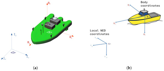
Figure 1.
Coordinate systems used in the modeling of USV dynamics. (a) Inertial and body-fixed frames for the USV. (b) Relationship between NED and body-fixed frames.
In maritime systems, a local tangent-plane approximation of the Earth is commonly adopted, wherein the inertial frame follows the North–East–Down (NED) convention. In this convention, the axes of the inertial frame point toward geographic north, east, and vertically downward, respectively. This convention is widely used due to its compatibility with compass-based navigation systems. In surface vehicle applications, the NED frame is typically assumed to coincide with the inertial frame , as the operating environment is locally bounded. This relationship is illustrated in Figure 1b.
To transform a vector from the inertial frame to the body-fixed frame , a rotation is applied using the Euler angles. The corresponding rotation matrix results from the sequential multiplication of three elemental rotation matrices. The specific order of multiplication depends on the chosen Euler angle convention, such as the ZYX sequence commonly used in marine applications.
3.2. Generalized Dynamic Model
For a system with n degrees of freedom, the dynamics are obtained from the Euler–Lagrange formulation. The configuration vector is defined as , where represents the translational components and the rotational components, such that . The Lagrangian is , where the kinetic energy is expressed as
leading to the generalized mass–inertia matrix
Applying the Euler–Lagrange equations yields the standard form:
where includes Coriolis and centrifugal terms, as well as the conservative forces, such as gravity or buoyancy.
Adding empirical velocity-dependent damping , and separating control from disturbances, the compact dynamic model becomes
3.3. Simplified Dynamic Model
Starting from the general Euler–Lagrange dynamics, we particularize the model to a 3-DOF representation in the inertial frame, where the state vector is defined as
with denoting the horizontal position of the vehicle and its yaw angle. The corresponding velocity vector is .
For surface vehicle models, the mass matrix is typically considered constant, and vertical dynamics are not included in this reduced space. Under these assumptions, the dynamics in the inertial frame reduce to the following:
To represent the vehicle’s motion relative to its own structure, the velocities are expressed in a body-fixed frame. The mapping between inertial and body-fixed velocities is defined by the following:
where
and denotes the surge, sway, and yaw rate in the body-fixed frame.
Finally, the dynamics expressed in the body-fixed frame are as follows:
3.4. Fossen’s Model
Following this formulation, the USV dynamics are represented using the structured model proposed by Fossen [27], whose main components are as follows:
where m is the vehicle mass, is the yaw moment of inertia, and are added mass terms. The linear damping coefficients are and , while and represent the quadratic damping terms. The generalized input vector is where and are the surge force, sway force, and yaw moment, respectively.
3.5. LQS-Based Parameter Estimation
From this representation, the system can be arranged into a regression form:
where is the regressor matrix and is the vector of unknown parameters to be estimated (see Table 1), leading to the following formulation:
with each sample defined as follows:

Table 1.
Estimated parameters.
The least-squares estimate of is obtained as follows:
where denotes the Moore–Penrose pseudoinverse.
3.6. System Identification
System identification is necessary because, although the rigid-body parameters of the USV are initially defined in the URDF model (e.g., mass, inertia), the final dynamic behavior results from its interaction with hydrodynamic plugins and environmental forces such as wind. These interactions introduce additional effects that are not directly accessible to the user. The identification workflow (Figure 2) begins with the design of persistently exciting inputs applied to each thruster so that the relevant surge–sway–yaw dynamics are sufficiently stimulated. We employ a variety of excitation patterns to span the target bandwidth. For each discrete time step k, timing indicators, such as rise time () and ultimate period (), are computed and logged. The resulting time series are then filtered and preprocessed to mitigate measurement noise and numerical artifacts.
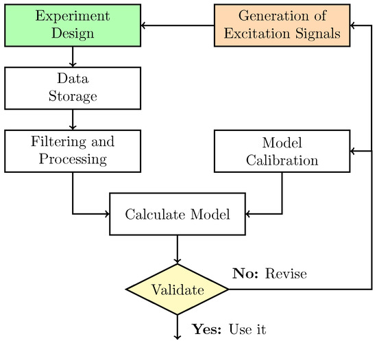
Figure 2.
USV identification pipeline: excitation design, data preprocessing, parameter estimation, and validation.
Given the cleaned dataset, a parametric 3-DOF model is estimated using a least-squares criterion. This method was selected due to its low computational cost and practical implementation, and is particularly suitable for academic and educational environments.
It is important to note that although the control-oriented modeling is performed in 3 degrees of freedom, the USV remains a 6-DOF operational platform. The vertical motion, roll, and pitch are fully simulated within the Gazebo environment. While the robot is underactuated and cannot directly control these additional DOFs, it can still perform tasks that depend on them, such as wave monitoring or rollover prevention.
4. Simulation Platform
This section covers the key elements of the simulation platform, including interface, communication, environmental models, sensors, and ROS framework design.
4.1. Graphical Interaction and Inter-Process Communication
This section describes each step involved in developing the USV visualization interface, focusing on graphical interaction and the setup of inter-process communication. These processes are supported by various components, including simulation modules, custom plugins, execution scripts, and configurable parameters. Additional details are provided in Figure 3.
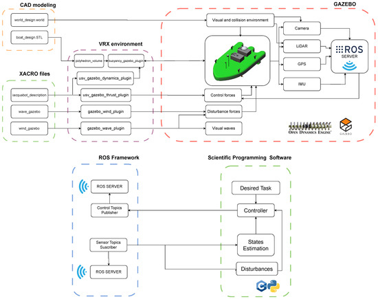
Figure 3.
Open-access simulator scheme.
The development process begins with the creation of a 3D model of the vessel using CAD software to capture its geometry. Additionally, the simulation world is designed, including both visual appearance and collision surfaces.
In parallel, the necessary simulation parameters are added to the XACRO files, including the vessel’s dynamic properties, such as mass, inertia, added mass, and hydrodynamic damping, as well as configuration settings for wave and wind effects. These files also define the robot’s physical structure, links, joints, visual elements, and sensor placements.
The parameters defined in the XACRO files are processed by the VRX plugins during simulation launch. These plugins initialize the vehicle dynamics and environmental conditions based on the provided configuration. As the simulation runs, the corresponding physical states are published to various Gazebo topics.
Subsequently, in the Gazebo simulator, all dynamic states continuously published on native Gazebo topics are integrated with the ODE physics engine to visually represent the robot’s physical behavior and its interaction with the environment. Various sensors are added through Gazebo’s native plugins. Finally, a clean communication layer is established with the ROS server, where sensor and actuator topics are published for further processing and control.
The final stages of the simulator focus on integration with the ROS framework, whose modular architecture allows for the simultaneous execution of multiple tasks and facilitates communication between components by defining a standard for published and subscribed messages. Controller implementation is incorporated into the sub-module named “Scientific Programming Software.” In this case, C++ and Python were used to generate ROS nodes directly within their respective environments.
4.2. USV Characterization
While the VRX WAM-V serves as the baseline, its physical and dynamic parameters (such as mass distribution, damping coefficients, and thrust response), were modified to represent the characteristics of a new monohull vessel developed for this project. The simulated USV is based on a real prototype constructed from a SEAFLO SF-S003 surfboard SEAFLO (Xiamen Doofar Outdoor Co., Ltd., Xiamen, China) () with a total mass of , modeled in SolidWorks 2022 SP0.0 and exported to the Gazebo-compatible Collada (DAE) format via STL conversion.
Propulsion is provided by four symmetrically mounted BlueRobotics T200 thrusters (Blue Robotics Inc., Redondo Beach, CA, USA) in a differential configuration (two forward, two aft). The thrust response is modeled as a nonlinear function of the input command , as defined in Equation (16). Model parameters were calibrated to match the T200 manufacturer curves [28], as shown in Table 2 and Figure 4.
Table 2.
Optimized parameters for the thrust model.
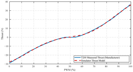
Figure 4.
Simulated thrust response vs. manufacturer data for T200 thrusters.
The simulated USV includes a set of simulated sensors integrated using ROS and Gazebo plugins. These include an IMU and GPS, a monocular RGB camera, a 3D LIDAR, and an acoustic pinger. Sensor parameters such as frequency, resolution, and noise were configured to reflect typical real-world devices and are easily adjustable through the XACRO model.
4.3. Wind Force
The wind force vector acting on the USV is expressed as follows:
where and are the frontal and lateral projected areas of the USV, respectively, L is the vessel length, is the relative wind attack angle, q is the dynamic pressure, and , , and are wind force coefficients. These terms are computed as follows:
where is the air density, is the relative wind speed, and , , and are empirical coefficients, typically within the ranges: , , and .
Given the true wind speed , true wind direction , surge and sway velocities u and v, and the USV’s yaw angle , the components of the relative wind velocity in the body-fixed frame are computed as follows:
Accordingly, the magnitude of the relative wind speed and the relative attack angle are given by the following:
4.4. Wave Model
The sea surface is modeled using the Gerstner wave formulation, which is widely applied in ocean simulations and computer graphics due to its capability to generate realistic wave patterns. Compared to simple sinusoidal models, Gerstner waves provide sharper crests and broader troughs, enhancing both visual and physical realism. The wave field is described as the superposition of N trochoidal wave components, following the 3D Gerstner wave formulation presented in [20], expressed as follows:
where denotes the initial position of a water particle, and and represent the steepness, amplitude, direction, wave number, angular frequency, and phase of the i-th wave component, respectively.
4.5. ROS Node and Topic Design
The following describes the distribution of ROS-based nodes and topics within the VRX simulation environment, as shown in Figure 5:
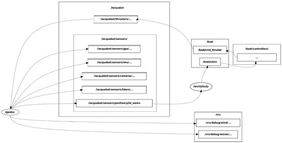
Figure 5.
ROS graph of topic-node communication in the Iacquabot simulation platform.
- Environmental Topics: Includes /vrx/debug/wind/speed and /vrx/debug/wind/direction for wind parameters, along with other topics related to ocean dynamics. Additionally, wave parameters, such as period, magnitude, and direction, are predefined in the simulation launch files (XACROs).
- Sensor Topics: Consist of GPS data on /iacquabot/sensors/gps/gps/fix, IMU measurements on /iacquabot/sensors/imu/imu/data, LiDAR point clouds on /iacquabot/sensors/lidars/lidar_wamv/points, and raw images from the front camera on /iacquabot/sensors/cameras/front_camera/image_raw.
- Actuation Topics: Commands for individual thrusters are published on topics such as /iacquabot/thrusters/right_front_thrust_cmd and /iacquabot/thrusters/right_rear_thrust_cmd. A high-level command topic /boat/cmd_thruster receives overall thruster commands, which are then translated into individual thruster inputs.
- State Estimation Topic: A custom C++ node, world2body.cpp, transforms velocity data from the inertial frame to the body frame. It publishes an odometry message on /boat/odom, containing position in the inertial frame and velocities in the body frame.
The complete specification of the onboard sensors, including their configuration parameters and implementation details, is provided in Appendix A.
5. Control Algorithm Formulation
This section presents the formulation of control algorithms, including velocity control, position control, trajectory tracking, and path guidance strategies.
5.1. Velocity Control
The velocity control module tracks a desired body-frame velocity vector by computing appropriate thrust commands for the port and starboard thrusters of the USV. Operating at , the controller uses a model-based proportional-derivative (PD) approach. The desired acceleration is estimated via finite differences:
A PD-like control input is then computed as follows:
where is a diagonal gain matrix.
Using the identified dynamics of the vehicle, the generalized force vector is obtained as follows:
The resulting surge force and yaw torque are converted into left and right thrust commands using a differential drive model:
Finally, each thrust command is mapped through the inverse of the nonlinear actuator model to generate the appropriate control inputs.
5.2. Position Control
The position controller drives the USV toward a desired position using a simple kinematic control law based on the current pose in the plane [29].
Let be the desired position and the current position of the vehicle. The orientation of the vehicle is given by the heading angle . The position error is defined as follows:
If the norm is less than a threshold (e.g., ), the controller outputs zero velocity. Otherwise, the desired heading is computed as follows:
where and are the components of .
The heading error is as follows:
The forward and angular velocities and are then calculated using proportional control laws:
where and are proportional gains for position and orientation errors, respectively. These gains can be tuned to adjust the controller’s behavior: for example, increasing relative to makes the vehicle prioritize alignment with the target heading before moving forward. The control signals are saturated according to predefined limits and .
5.3. Trajectory Tracking
A trajectory-tracking controller is implemented to guide the USV along a time-varying reference path. The reference trajectory is first defined as a continuous function of time, and its time derivatives (velocities) are computed in continuous time. Both the position and velocity trajectories are then discretized by evaluating them at a fixed sampling interval over a predefined time horizon, resulting in sequences of desired positions and velocities indexed by discrete time steps.
Let denote the desired time-varying pose and its time derivative, while represents the current pose of the USV. The tracking error in the global frame is computed in discrete time as follows:
The corrected velocity in the inertial frame is obtained by adding proportional feedback to the nominal reference:
This velocity is transformed into the body-fixed frame to compute the control input:
where a is the look-side distance.
5.4. Path Guidance
Finally, a path guidance controller is implemented to steer the USV along a predefined geometric path. Unlike trajectory tracking, where both position and velocity are time-parametrized as and , in paths, following the path is defined as a curve:
where s is a spatial parameter. The reference velocity is defined according to application requirements, while the desired position is chosen as the projection of the current position onto the path:
with
Once is obtained, the position error and the corrected inertial velocity are computed following the same approach described in the trajectory tracking controller, and the control inputs and are obtained using the same transformation to the body-fixed frame.
6. Simulation Results
The system parameters were identified using a Least Squares approach. In addition to the point estimates, we also computed the 95% confidence intervals (CI) and the standard deviations (STD) of the estimates, in order to quantify both the accuracy and the uncertainty of the identified values. These results are summarized in Table 3. Model validation was performed by comparing the body velocities predicted by the identified model against the measured data, as illustrated in Figure 6a. The input signals used for identification and validation are provided in Appendix B.
Table 3.
Identified parameters for USV, 95% confidence intervals (CI), and standard deviations (STD).
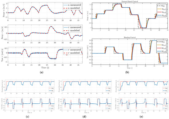
Figure 6.
(a) Comparison between measured data and the predicted body velocities (u, v, r). (b) Velocity control response (u and w) under three disturbance scenarios. (c–e) Velocity control validation for scenarios 1, 2, and 3, respectively.
Table 4 presents the quantitative validation metrics of the identified 3-DOF dynamic model of the USV. The table reports the root mean squared error (RMSE), mean absolute error (MAE), and coefficient of determination () for each velocity and pose component. These values indicate that the identified model reproduces the measured trajectories with high accuracy, with values above 0.99 in all states.
Table 4.
Validation metrics (RMSE, MAE, and ) for the identified dynamic model of USV.
To evaluate the USV dynamics and the impact of environmental disturbances, three scenarios were considered: (i) vehicle dynamics with no external disturbances, where only hydrodynamic interaction is present; (ii) dynamics under wave disturbances; and (iii) combined wave and wind disturbances.
The performance of the velocity controller was evaluated by tracking varying desired surge () and sway () velocities under the three disturbance scenarios previously described. Following the PD-like control law, the gain matrix was defined as . The resulting velocity responses, which validate the controller’s performance, are presented in Figure 6b. Quantitative results of the controller accuracy are reported in Table 5.
Table 5.
Validation metrics (RMSE, MAE, and ) for the velocity control experiments of the USV.
For position control, a circuit composed of six waypoints was defined to evaluate the USV’s ability to follow a predefined route under the three disturbance scenarios. The route followed in each scenario is illustrated in Figure 7, while the corresponding velocity responses are shown in Figure 6c–e.
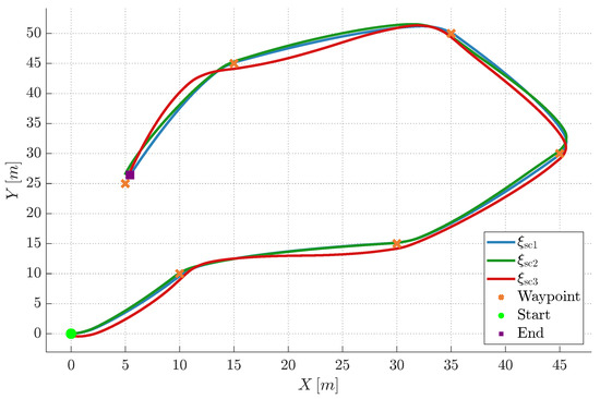
Figure 7.
Route followed by the USV in the three scenarios over the six-waypoint circuit.
A set of sinusoidal, circular, and spiral reference trajectories was established to test the USV’s trajectory-tracking performance, as listed in Table 6. Each of these trajectories was performed under the three disturbance scenarios to analyze the controller’s behavior. The experimental results, including the paths followed and the corresponding velocity tracking errors, are shown in Figure 8. Table 7 provides the quantitative validation of these runs, confirming sub-meter RMSE and above 0.91 in all cases.
Table 6.
Reference trajectories for the USV.
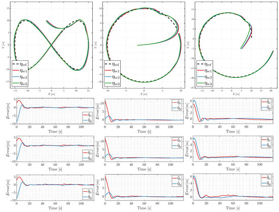
Figure 8.
Trajectory tracking results and tracking error for three experiments under different environmental conditions. (Row 1): Trajectories of Experiments 1–3 (desired vs. real). (Row 2): Tracking error under no disturbance. (Row 3): Tracking error under wave conditions. (Row 4): Tracking error under combined wave and wind.
Table 7.
Validation metrics (RMSE, MAE, and ) for trajectory-tracking experiments of the USV.
Finally, the path-following controller was evaluated by analyzing the path error and velocity tracking error when following a diagonal reference path defined as . A constant reference velocity was imposed to assess the controller’s ability to maintain the desired surge speed while minimizing cross-track deviations. Five experiments were performed using different initial positions and headings, as well as varying disturbance forces and directions, as summarized in Table 8. The resulting path-following and velocity errors obtained in these experiments are presented in Figure 9, highlighting the robustness and convergence properties of the proposed controller.
Table 8.
Initial conditions and disturbances for the five path-following experiments.
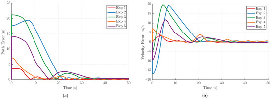
Figure 9.
Path-following and velocity-tracking errors obtained from the five path-following experiments with different initial conditions and disturbance forces (see Table 8). (a) Path-following error for the five experiments. (b) Velocity-tracking error for the five experiments.
Regarding computational performance, the simulations were executed on a workstation running Ubuntu 20.04 equipped with an AMD Ryzen 5 5400 processor and 16 GB of RAM. In Gazebo, the average real-time factor (RTF) was between 0.95 and 1.0, with an average frame rate of 67 FPS. When visualization through RViz was enabled, the RTF decreased slightly to 0.92–0.95, while the frame rate dropped to approximately 43 FPS. All controllers and sampling processes were designed to operate at 50 Hz and showed no degradation in performance under these computational conditions.
7. Analysis of Result
This paper introduced an open-access simulation and control development platform for surface robotic vehicles, extending the capabilities of the VRX environment. The platform integrates a fully open-source testing framework that combines vehicle modeling, thruster characterization, and multi-mode motion controllers into a single environment. A kayak-type monohull USV with a differential configuration of four thrusters, two at the bow and two at the stern, was implemented as a mockup, both in its graphical design and dynamic model. The propulsion system was modeled using a thrust-mapping function calibrated against manufacturer-provided data, while the vehicle dynamics were identified using a simplified 3-DOF Fossen-based model and Least Squares estimation.
An important aspect of the modeling results is that the VRX simulator itself uses a 6-DOF dynamic model inspired by Fossen’s formulation. This structural consistency explains why the identified 3-DOF Fossen model showed such a close match with the simulated data, as observed in the velocity validation (Figure 6a). Although inertial sensors in the simulation include noise, the validation response appears nearly ideal. In real-world applications, however, identification and validation experiments would need to be conducted in controlled environments with minimal disturbances, and even then, the modeling would not be perfect. In such cases, approaches such as data-driven modeling or unknown dynamics compensation through neural networks could be employed to complement classical physics-based models.
The suite of motion controllers developed in this work was designed to evaluate different operational tasks. The velocity controller, following the PD-like law , was tested under three disturbance scenarios (Figure 6b). Due to the differential thruster configuration, the USV cannot simultaneously reach its maximum surge speed u and yaw rate . For this reason, the velocity control tests sought a balance between surge and yaw performance by adjusting the gains of .
In position control experiments, the priority was shifted toward yaw () rather than surge speed, since the primary objective was reaching a waypoint regardless of time. This strategy allowed the USV to orient itself toward the next waypoint before advancing. Additionally, a tolerance zone around each waypoint was essential to avoid oscillatory or unstable behavior, especially under disturbances. In contrast, for trajectory tracking tasks (Table 6), the controller prioritized surge velocity u over orientation, as the reference path was time-parametrized and the vehicle needed to follow the moving reference closely rather than correcting heading errors first.
From a practical standpoint, path following is often the most relevant task for USVs, particularly in applications such as bathymetric mapping, infrastructure inspection, or search missions. In the experiments performed (Table 8, Figure 9), it was observed that the USV adapted its heading to compensate for the direction of the disturbance forces, effectively “leaning” against the disturbance to maintain the desired path. This behavior highlights the platform’s ability to emulate realistic navigation scenarios where maintaining a path is more critical than precise trajectory tracking.
Beyond the evaluation of control strategies, the platform itself is a key contribution of this work. The open-source design and modularity enable quick adaptation to different vehicle configurations and testing conditions. This aligns with the overarching goal of creating a reproducible and extensible testing environment rather than a digital twin of a single real-world USV.
Limitations and Future Work
Although the kayak-type mockup was inspired by real USV designs, the present work does not attempt to construct a full digital twin of a physical platform. Instead, the contribution lies in providing the scientific community with an open-access and extensible simulation framework, including realistic geometries, actuator response curves, and communication interfaces, that can be adapted to diverse USV configurations. Future research will focus on applying systematic methodologies for digital model validation, such as the procedure described in [30], to progressively increase the platform’s fidelity with respect to real-world behavior.
In terms of control, the present article did not seek to propose a novel or sophisticated law but to demonstrate how the platform can support multiple architectures for tasks such as velocity regulation, trajectory tracking, and path following. In future work, more advanced controllers will be investigated, including robust designs based on and -synthesis [31], which explicitly account for uncertainties and unmodeled disturbances. Model Predictive Control (MPC) will also be explored not only for multi-variable optimization but also for enabling safe path-following tasks using control barrier functions and contouring control formulations [32,33], as well as for investigating fault-tolerant robust controllers [34,35].
Furthermore, since the simulator has been developed in Gazebo and is fully open access, it can be easily extended to incorporate additional robots for multi-agent scenarios. This feature enables the exploration of cooperative control strategies between USVs and UAVs [36], as well as dynamic interaction with other mobile USVs, such as collision avoidance and cooperative navigation tasks in complex marine environments.
Additionally, the integration of sensor-based strategies, such as visual servoing and LiDAR-based obstacle detection and avoidance, will be implemented to assess the platform as a realistic proving ground for autonomous navigation and high-level control design in challenging marine environments. These planned extensions will continue to strengthen the platform as a community resource for marine robotics research and graduate education.
8. Conclusions
This work introduced an open-access testing framework that extends the VRX environment with a customizable monohull USV mockup, a simplified dynamic model identified via Least Squares, and a suite of motion controllers evaluated under realistic disturbance scenarios. The main outcome of this effort is not only the validation of the implemented control strategies but the delivery of a modular and reproducible platform that can serve as a foundation for future developments in surface robotics.
From the conducted experiments, several insights were gained regarding controller design and vehicle behavior. Due to the differential thruster configuration, the trade-off between surge velocity and yaw rate must be carefully managed, with different priorities depending on the control task (velocity, position, trajectory, or path following). Path following, which is of particular relevance for real-world USV operations such as mapping or infrastructure inspection, proved to be the most natural and effective control mode, showing the vehicle’s ability to adapt its heading to counteract external forces and maintain the desired path.
The platform is fully open-source and scalable, enabling straightforward integration of other vehicle models or alternative control architectures. Future efforts will build upon this foundation to explore advanced model-based approaches, such as MPC, and sensor-driven methods, including vision-based servoing and LiDAR-based obstacle detection, thereby strengthening the platform’s role as a versatile testbed for autonomous marine navigation.
These sensor configurations provide a balanced trade-off between realism and computational efficiency, ensuring that the proposed simulation framework remains accessible to the community while capturing key aspects of sensor uncertainty in marine robotics experiments.
Author Contributions
Conceptualization, B.S.-M. and J.M.; methodology, B.S.-M.; software, B.S.-M.; validation, B.S.-M., F.R., and J.M.T.; formal analysis, B.S.-M., F.R., and J.M.T.; data curation, B.S.-M. and D.B.; writing—original draft preparation, B.S.-M.; writing—review and editing, J.M., D.B., F.R., and J.M.T.; visualization, D.B.; supervision, F.R. and J.M.T.; project administration, F.R. and J.M.T.; funding acquisition, J.M. All authors have read and agreed to the published version of the manuscript.
Funding
This research was funded by the Instituto de Automática of the Universidad Nacional de San Juan in collaboration with CONICET (Consejo Nacional de Investigaciones Científicas y Técnicas).
Data Availability Statement
The data supporting the findings of this study, including the simulation platform, predefined control implementations, scenarios, and supplementary figures and videos, are openly available at https://github.com/BraJavSa/iacquabotsim (accessed on 15 October 2025). Further inquiries can be directed to the corresponding author.
Acknowledgments
I would like to express my sincere gratitude to the National Scientific and Technical Research Council (CONICET) and the German Academic Exchange Service (DAAD) for their financial support, which made this research possible. I am also thankful to the Automatics Institute and the Faculty of Engineering for providing an excellent academic and research environment. During the preparation of this manuscript, the author used DeepL (web version) for the purposes of minor language polishing.
Conflicts of Interest
The authors declare no conflicts of interest.
Abbreviations
The following abbreviations are used in this manuscript:
| USV | Unmanned Surface Vehicle |
| VRX | Virtual RobotX (simulation for autonomous vehicle competitions) |
| WAM-V | Wave Adaptive Modular Vessel |
| UAV | Unmanned Aerial Vehicle |
| UGV | Unmanned Ground Vehicle |
| LQS | Least Quadratic Squares |
| DOF | Degrees of Freedom |
| ROS | Robot Operating System |
| IMU | Inertial Measurement Unit |
| LiDAR | Light Detection and Ranging |
| DAE | Digital Asset Exchange (Collada format) |
| MiTL | Model-in-the-Loop |
| UUV | Unmanned Underwater Vehicle |
Appendix A
All onboard sensors of the simulated USV were modeled in Gazebo to emulate their real-world counterparts. Each parameter can be modified in iacquabotsim/usv_gazebo/urdf/ components/sensor_name.xacro. Table A1, Table A2, Table A3, Table A4 and Table A5 summarize the configuration used in this work.
Table A1.
Configuration of the simulated monocular camera.
Table A1.
Configuration of the simulated monocular camera.
| Parameter | Value | Units |
|---|---|---|
| Resolution | pixels | |
| Horizontal FOV | 80 | deg |
| Range | 0.05–300 | m |
| Update rate | 30 | Hz |
| Noise (std. dev.) | 0.007 | – |
Table A2.
Configuration of the simulated 3D LiDAR.
Table A2.
Configuration of the simulated 3D LiDAR.
| Parameter | Value | Units |
|---|---|---|
| Horizontal FOV | 360 | deg |
| Vertical FOV | to | deg |
| Horizontal resolution | 0.1 | deg |
| Vertical layers | 6 | – |
| Max. range | 70 | m |
| Update rate | 20 | Hz |
| Noise (std. dev.) | 0.002 | m |
Table A3.
Configuration of the simulated GPS.
Table A3.
Configuration of the simulated GPS.
| Parameter | Value | Units |
|---|---|---|
| Update rate | 15 | Hz |
| Position noise (std. dev.) | 0.5 | m |
| Velocity noise (std. dev.) | 0.05 | m/s |
| Coordinate frame | NWU | – |
Table A4.
Configuration of the simulated IMU.
Table A4.
Configuration of the simulated IMU.
| Parameter | Value | Units |
|---|---|---|
| Update rate | 15 | Hz |
| Accel. noise (std. dev.) | 0.01 | |
| Gyro noise (std. dev.) | 0.01 | rad/s |
| Yaw drift frequency | Hz |
Table A5.
Configuration of the echosounder.
Table A5.
Configuration of the echosounder.
| Parameter | Value | Units |
|---|---|---|
| Range | 0.2–50 | m |
| Update rate | 1 | Hz |
| Noise (std. dev.) | 0.01 | m |
Appendix B

Figure A1.
Command (CMD) signals sent to the left and right thrusters during the system identification experiments. (a) Identification signals, designed to explore the vessel’s full dynamic range. (b) Independent validation signals, used to test how well the identified model can predict the vessel’s behavior.
References
- Zereik, E.; Bibuli, M.; Mišković, N.; Ridao, P.; Pascoal, A. Challenges and future trends in marine robotics. Annu. Rev. Control 2018, 46, 350–368. [Google Scholar] [CrossRef]
- Liu, Z.; Zhang, Y.; Yu, X.; Yuan, C. Unmanned surface vehicles: An overview of developments and challenges. Annu. Rev. Control 2016, 41, 71–93. [Google Scholar] [CrossRef]
- Heins, P.H.; Jones, B.L.; Taunton, D.J. Design and validation of an unmanned surface vehicle simulation model. Appl. Math. Model. 2017, 48, 749–774. [Google Scholar] [CrossRef]
- Choi, H.; Crump, C.; Duriez, C.; Elmquist, A.; Hager, G.; Han, D.; Hearl, F.; Hodgins, J.; Jain, A.; Leve, F.; et al. On the use of simulation in robotics: Opportunities, challenges, and suggestions for moving forward. Proc. Natl. Acad. Sci. USA 2021, 118, e1907856118. [Google Scholar] [CrossRef] [PubMed]
- Takaya, K.; Asai, T.; Kroumov, V.; Smarandache, F. Simulation Environment for Mobile Robots Testing Using ROS and Gazebo. In Proceedings of the 2016 20th International Conference on System Theory, Control and Computing (ICSTCC), Sinaia, Romania, 13–15 October 2016; pp. 2149–2154. [Google Scholar] [CrossRef]
- Rohmer, E.; Singh, S.P.; Freese, M. V-REP: A Versatile and Scalable Robot Simulation Framework. In Proceedings of the IEEE/RSJ International Conference on Intelligent Robots and Systems (IROS), Tokyo, Japan, 3–7 November 2013; pp. 1321–1326. [Google Scholar] [CrossRef]
- Pebrianti, D.; Suhaimi, M.S.; Bayuaji, L.; Hossain, M.J. Exploring Micro Aerial Vehicle Mechanism and Controller Design Using Webots Simulation. Mekatronika 2023, 5, 41–49. [Google Scholar] [CrossRef]
- Shah, S.; Dey, D.; Lovett, C.; Kapoor, A. AirSim: High-fidelity Visual and Physical Simulation for Autonomous Vehicles. In Proceedings of the Field and Service Robotics, Zurich, Switzerland, 12–15 September 2017; pp. 621–635. [Google Scholar] [CrossRef]
- Varela-Aldás, J.; Recalde, L.F.; Guevara, B.S.; Andaluz, V.H.; Gandolfo, D.C. Open-Access Platform for the Simulation of Aerial Robotic Manipulators. IEEE Access 2024, 12, 49735–49751. [Google Scholar] [CrossRef]
- Campbell, S.; Naeem, W.; Irwin, G. A review on improving the autonomy of unmanned surface vehicles through intelligent collision avoidance manoeuvres. Annu. Rev. Control 2012, 36, 267–283. [Google Scholar] [CrossRef]
- Ashrafiuon, H.; Muske, K.R.; McNinch, L.C.; Soltan, R.A. Sliding-mode tracking control of surface vessels. IEEE Trans. Ind. Electron. 2008, 55, 4004–4012. [Google Scholar] [CrossRef]
- Lv, C.; Yu, H.; Hua, Z.; Li, L.; Chi, J. Speed and Heading Control of an Unmanned Surface Vehicle Based on State Error PCH Principle. Math. Probl. Eng. 2018, 2018, 7371829. [Google Scholar] [CrossRef]
- Silva-Sassaman, D.; Jeong, M.; Sassaman, P.; Wu, Z.; Li, A.Q. CataBotSim: A Realistic Aquatic Simulator for Autonomous Surface Vehicle Testing. In Proceedings of the 2024 Eighth IEEE International Conference on Robotic Computing (IRC), Tokyo, Japan, 11–13 December 2024; pp. 202–209. [Google Scholar] [CrossRef]
- Hu, J.; Yang, X.; Lou, M.; Wang, Q.; Ye, H.; Liu, W. Virtual-reality-based design and implementation with a parallel physical simulation platform for unmanned surface vehicle. In Proceedings of the 2023 International Conference on Cyber-Physical Social Intelligence (ICCSI), Xi’an, China, 20–23 October 2023; pp. 262–267. [Google Scholar] [CrossRef]
- Chaudhary, A.; Mishra, R.; Kalyan, B.; Chitre, M. Development of an Underwater Simulator using Unity3D and Robot Operating System. In Proceedings of the OCEANS 2021: San Diego—Porto, San Diego, CA, USA, 20–23 September 2021; pp. 1–7. [Google Scholar] [CrossRef]
- Potokar, E.; Ashford, S.; Kaess, M.; Mangelson, J.G. HoloOcean: An Underwater Robotics Simulator. In Proceedings of the 2022 International Conference on Robotics and Automation (ICRA), Philadelphia, PA, USA, 23–27 May 2022; pp. 3040–3046. [Google Scholar] [CrossRef]
- Cieslak, P. Stonefish: An Advanced Open-Source Simulation Tool Designed for Marine Robotics, with a ROS Interface. In Proceedings of the OCEANS 2019—Marseille, Marseille, France, 17–20 June 2019; pp. 1–6. [Google Scholar] [CrossRef]
- Manhaes, M.M.M.; Scherer, S.A.; Voss, M.; Douat, L.R.; Rauschenbach, T. UUV Simulator: A Gazebo-based package for underwater intervention and multi-robot simulation. In Proceedings of the OCEANS 2016 MTS/IEEE Monterey, Monterey, CA, USA, 19–23 September 2016; pp. 1–8. [Google Scholar] [CrossRef]
- Loncar, I.; Obradovic, J.; Krasevac, N.; Mandic, L.; Kvasic, I.; Ferreira, F.; Slosic, V.; Nad, D.; Miskovic, N. MARUS—A Marine Robotics Simulator. In Proceedings of the OCEANS 2022, Hampton Roads, VA, USA, 17–20 October 2022; pp. 1–7. [Google Scholar] [CrossRef]
- Bingham, B.; Aguero, C.; McCarrin, M.; Klamo, J.; Malia, J.; Allen, K.; Lum, T.; Rawson, M.; Waqar, R. Toward Maritime Robotic Simulation in Gazebo. In Proceedings of the OCEANS 2019 MTS/IEEE SEATTLE, Seattle, WA, USA, 27–31 October 2019; pp. 1–10. [Google Scholar] [CrossRef]
- Campos, D.F.; Matos, A.; Pinto, A.M. Multi-domain inspection of offshore wind farms using an autonomous surface vehicle. SN Appl. Sci. 2021, 3, 455. [Google Scholar] [CrossRef]
- Wu, X.; Wei, C. DRL-Based Motion Control for Unmanned Surface Vehicles with Environmental Disturbances. In Proceedings of the 2023 IEEE International Conference on Unmanned Systems (ICUS), Hefei, China, 13–15 October 2023; pp. 1696–1700. [Google Scholar] [CrossRef]
- Bayrak, M.; Bayram, H. COLREG-Compliant Simulation Environment for Verifying USV Motion Planning Algorithms. In Proceedings of the OCEANS 2023—Limerick, Limerick, Ireland, 5–8 June 2023; pp. 1–10. [Google Scholar] [CrossRef]
- Li, J.; Chavez-Galaviz, J.; Azizzadenesheli, K.; Mahmoudian, N. Dynamic Obstacle Avoidance for USVs Using Cross-Domain Deep Reinforcement Learning and Neural Network Model Predictive Controller. Sensors 2023, 23, 3572. [Google Scholar] [CrossRef]
- Chen, L.; Liu, C.; Guo, S.; Qian, H. Vision-Guided UAV Landing on a Swaying Ocean Platform in Simulation. In Proceedings of the 2023 IEEE International Conference on Real-Time Computing and Robotics (RCAR), Datong, China, 17–20 July 2023; pp. 456–462. [Google Scholar] [CrossRef]
- Lu, S.; Wang, B.; Dong, Z.; Hu, Z.; Ding, Y.; Liu, W. Parameter Identification of an Unmanned Surface Vessel Nomoto Model Based on an Improved Extended Kalman Filter. Appl. Sci. 2024, 15, 161. [Google Scholar] [CrossRef]
- Fossen, T.I. Handbook of Marine Craft Hydrodynamics and Motion Control; Wiley: Hoboken, NJ, USA, 2011. [Google Scholar] [CrossRef]
- Blue Robotics Inc. T200 Thruster: ROV Thruster for Marine Robotics Propulsion. Available online: https://bluerobotics.com/store/thrusters/t100-t200-thrusters/t200-thruster-r2-rp/ (accessed on 16 August 2025).
- Carelli, R.; Secchi, H.; Mut, V. Algorithms for stable control of mobile robots with obstacle avoidance. Lat. Am. Appl. Res. 1999, 29, 191–196. [Google Scholar]
- Saldarriaga-Mesa, B.; Varela-Aldás, J.; Roberti, F.; Toibero, J.M. A Novel Methodology for Designing Digital Models for Mobile Robots Based on Model-Following Simulation in Virtual Environments. Robotics 2025, 14, 124. [Google Scholar] [CrossRef]
- Hui, N.; Guo, Y.; Han, X.; Wu, B. Robust H-Infinity Dual Cascade MPC-Based Attitude Control Study of a Quadcopter UAV. Actuators 2024, 13, 392. [Google Scholar] [CrossRef]
- Ma, Y.; Liu, Z.; Wang, T.; Song, S.; Xiang, J.; Zhang, X. Multi-model predictive control strategy for path-following of unmanned surface vehicles in wide-range speed variations. Ocean Eng. 2024, 295, 116845. [Google Scholar] [CrossRef]
- Lei, T.; Wen, Y.; Yu, Y.; Tian, K.; Zhu, M. Predictive trajectory tracking control for the USV in networked environments with communication constraints. Ocean Eng. 2024, 298, 117185. [Google Scholar] [CrossRef]
- Meng, J.; Tan, H.; Jiang, L.; Qian, C.; Xiao, H.; Hu, Z.; Li, G. Robust finite-time sliding mode control of unmanned surface vehicle with active compensation of pose estimation uncertainty. Ocean Eng. 2024, 304, 117831. [Google Scholar] [CrossRef]
- Gonzalez-Garcia, A.; Castañeda, H.; De León-Morales, J. Unmanned surface vehicle robust tracking control using an adaptive super-twisting controller. Control Eng. Pract. 2024, 149, 105985. [Google Scholar] [CrossRef]
- Li, J.; Zhang, G.; Zhang, W.; Zhang, X. Robust control for cooperative path following of marine surface-air vehicles with a constrained inter-vehicles communication. Ocean Eng. 2024, 308, 118240. [Google Scholar] [CrossRef]
Disclaimer/Publisher’s Note: The statements, opinions and data contained in all publications are solely those of the individual author(s) and contributor(s) and not of MDPI and/or the editor(s). MDPI and/or the editor(s) disclaim responsibility for any injury to people or property resulting from any ideas, methods, instructions or products referred to in the content. |
© 2025 by the authors. Licensee MDPI, Basel, Switzerland. This article is an open access article distributed under the terms and conditions of the Creative Commons Attribution (CC BY) license (https://creativecommons.org/licenses/by/4.0/).