Article

Adaptive Path Planning for Subsurface Plume Tracing with an Autonomous Underwater Vehicle †

1
School of Mechanical Engineering, Tianjin University, Tianjin 300354, China
2
Yichang Research Institute of Testing Technology, Yichang 443003, China
3
China Automotive Technology and Research Center, Tianjin 300300, China
*
Author to whom correspondence should be addressed.
This paper is an extended version of our paper published in Bao Z, Li Y, Shao X et al. Adaptive Path Planning for Plume Detection with an Underwater Glider. In Mechanisms and Machine Science, Proceedings of the 16th IFToMM World Congress 2023, Tokyo, Japan, 5–10 November 2023; Springer: Cham, Switzerland; Heidelberg, Germany, 2015.
Robotics 2024, 13(9), 132; https://doi.org/10.3390/robotics13090132
Submission received: 30 June 2024 / Revised: 31 July 2024 / Accepted: 19 August 2024 / Published: 31 August 2024

Abstract

:
Autonomous underwater vehicles (AUVs) have been increasingly applied in marine environmental monitoring. Their outstanding capability of performing tasks without human intervention makes them a popular tool for environmental data collection, especially in unknown and remote regions. This paper addresses the path planning problem when AUVs are used to perform plume source tracing in an unknown environment. The goal of path planning is to locate the plume source efficiently. The path planning approach is developed using the Double Deep Q-Network (DDQN) algorithm in the deep reinforcement learning (DRL) framework. The AUV gains knowledge by interacting with the environment, and the optimal direction is extracted from the mapping obtained by a deep neural network. The proposed approach was tested by numerical simulation and on a real ground vehicle. In the numerical simulation, several initial sampling strategies were compared on the basis of survey efficiency. The results show that direct learning based on the interaction with the environment could be an appropriate survey strategy for plume source tracing problems. The comparison with the canonical lawnmower path used in practice showed that path planning using DRL algorithms could be potentially promising for large-scale environment exploration.

1. Introduction

Oil spills cause immediate and long-lasting damage to the marine environment and even adverse impacts on human health. An ecosystem-level injury to coastal and deepwater species, as well as their habitats, was declared as a result of the 2010 Deepwater Horizon oil spill [1]. This oil spill disaster is known as the largest spill in world history. Approximately 3.19 million barrels of crude oil were released into the ocean [2]. Most of the spilled oil moved upwards through the water column and formed oil slicks, floating on the water surface and extending over 43,300 square miles. Subsurface oil plumes were also observed and identified as a mixture of oil droplets and chemical dispersants via in situ sampling [3] and ingredient analysis [4].
Oil transport on the surface and in the water column is governed by a variety of physical, chemical, and biological processes. Oil slick detection and subsurface plume tracking can improve the understanding of oil movement and the associated effects of ocean circulation. While oil slicks can be observed by using synthetic aperture radar (SAR) images [5], tracing subsurface oil plumes is not straightforward [6]. In the Deepwater Horizon oil spill, chemical dispersants were injected into the oil flow near the wellhead as a response action. Small oil droplets were formed and retained in deep water as subsurface plumes at a 1000–1200 m water depth [4]. Such deepwater oil plumes, as well as the subsurface plumes resulting from the interaction between the oil slick and surface mixing processes, are not accessible for visual observation [7].
Autonomous underwater vehicles (AUVs) are regarded as the most relevant devices in geoscience studies that are targeted at the interface between the seabed and the water column [8]. Compared with conventional static sensors and manned platforms, AUVs are better suited for subsurface plume tracing in that they are more flexible in deployment and can operate autonomously in remote areas that might be hostile or dangerous to human beings. In the 2010 Deepwater Horizon oil spill disaster, a Sentry AUV was used to conduct subsurface sampling surveys to characterize deepwater oil plumes [7]. It was later revealed that underwater oil spills result in a significant fraction of hydrocarbons being retained in midwater [9]. Motivated by AUVs’ prominent performance in plume tracing during the Deepwater Horizon oil spill, Dipinto et al. equipped a Remus AUV (Woods Hole, MA, USA) with oil characterization sensors to leverage AUV technologies in oil spill responses [10], Hwang et al. established a control architecture for AUVs to monitor and determine undissolvable marine pollutants resulting from oil spills [11], and Gomez-lbanez et al. developed an AUV-based water sampling system for the autonomous detection and sampling of underwater oil plumes [12].
AUVs’ performance in plume tracing tasks greatly depends on their survey strategy. The most common strategy undertaken by AUVs in practice is to follow a preplanned lawnmower pattern [6,10]. This canonical survey path is usually adopted to achieve full coverage over a studied region. However, significant features of the subsurface plume may be missed because the location and extent of the plume are usually priorly unknown. Efforts have been made to optimize the survey strategies with which AUVs can plan the sampling path to the plume source.
An initial attempt in plume tracing was to calculate a concentration gradient [13]. But gradient-based algorithms are not practical for oil plume tracing because an oil plume is actually made up of droplets of oil with a discontinuous and patchy distribution in the marine environment [6,14]. Investigations have been carried out on applying biological behaviors to robotic path planning for plume tracing. The most widely used biomimetic strategies are based on olfactory sensing, which is used by animals to search for targets, such as food, nests, and mates. Farrell et al. presented a behavior-based planning algorithm for chemical plume tracing [15]. Motivated by the maneuvering behaviors of moths flying upwind along a pheromone plume, Li et al. designed a moth-inspired motion planning strategy for AUVs to trace the plume source [16]. Grasso and Atema explored a biological plume tracing strategy known as ‘odor-gated rheotaxis ’ that incorporates the sensing of the mean flow and chemical detection for guidance [17]. Bioinspired behavior-based algorithms generate reactive strategies. Fixed actions are executed repetitively. Hence, these approaches may not be compatible with complex environments [18].
As robotic technology advances, solutions including a group of robots have also been proposed as a promising approach to plume tracing [19,20,21]. The focus of these studies was the chemical plume tracing (CPT) problem in environment monitoring using ground-based or aerial vehicles. Plume source tracing in the underwater environment by multi-agent systems is intrinsically difficult because the ocean environment is highly dynamic and unstable [22]. Common multi-agent tracking approaches based on accurate feature modeling are usually not applicable [23]. Several recent studies were devoted to providing solutions for restricted communication [24], analyzing the collective behavior of multi-agent systems with various degrees of heterogeneity [25], and accelerating the learning process of multi-agent systems [26].
To achieve efficient plume source locating via multi-robot collaboration, the most essential issue is to develop intelligent survey strategies that can be extended for swarm applications. Pang and Farrell proposed a source-likelihood mapping approach based on the Bayesian inference method to locate the sources of chemicals in a turbulent fluid flow by estimating the source location based on the detection history [27]. Jiu et al. presented a path planning strategy based on Partially Observable Markov Decision Processes and the artificial potential field algorithm [28]. Other potential techniques include those having been applied in environmental monitoring, where the interests of detection are associated with the extreme values of the sampled variable [29]. Reinforcement learning approaches have also used to solve the plume tracing problem [18]. A long short-term memory based deterministic policy gradient algorithm was adopted to optimize the plume tracing strategy for an AUV in a turbulent environment. Wang and Pang proposed a deep reinforcement learning (DRL)-based fused algorithm to locate hydrothermal vents [30]. The DRL algorithm was utilized to learn the weight that is used to fuse the Bayesian-inference method and the moth-inspired method.
This paper presents a reinforcement-learning-based path planning approach for AUVs to locate the source of subsurface oil plumes. It is an extension of our previous work [31]. It is assumed that no prior knowledge of the plume is available, and the goal is to adaptively find the plume source location efficiently. In the presented approach, the plume tracing problem is modeled under the Markov Decision Process (MDP) framework, and the Double Deep Q-Network (DDQN) algorithm is used to learn an optimal survey path for AUVs. The main contributions of this work are as follows:
  • Illustration of the feasibility of applying adaptive path planning using the DDQN algorithm to plume tracing problems by numerical simulations.
  • Analysis of the superiority of the adaptive survey approach over the conventional lawnmower approach in terms of survey efficiency for large-scale exploration.
The remainder of this paper is organized as follows. Section 2 presents the problem formulation. The methods used to generate the adaptive survey path is addressed in Section 3. Section 4 and Section 5 present the simulation results and the experiments, respectively. Section 6 concludes this work, and Section 7 presents the future work.

2. Problem Formulation

The goal of subsurface oil plume tracing is to characterize plumes by locating their sources. An oil plume is defined as a spatial interval with hydrocarbon signals or signal surrogates and can be identified by in situ sensing of the anomalies in hydrocarbon signals [7]. When AUVs are deployed for plume tracing, as shown in Figure 1, the initial attempts as the first phase of the task follow sawtooth survey trajectories in the vertical dimension to determine the depth of these neutrally buoyant plumes [32]. Surveys at a constant depth are subsequently carried out in the second phase for plume source characterization. It is assumed that AUVs operate in a local area at approximately constant longitude and latitude, and a local Cartesian North-East-Down (NED) coordinate system is used.
This work focuses on the second phase, when AUVs survey at a constant depth in the water. It is assumed that no prior information about the location of the source and the chemical concentration distribution is available. Since the endurance of AUVs is limited by their onboard battery capacity, our aim is to develop an approach that can enable AUVs to automatically plan their survey path and efficiently locate the plume source.
AUVs start to survey the region of interest immediately after deployment. The survey path is formed by connecting successive waypoints. Therefore, waypoint determination is essential in AUV path planning.. During the course of plume tracing, sensors such as fluorometers are used to measure hydrocarbon concentrations [7] along AUVs’ track lines from the current waypoint to the next one. The waypoints can be preplanned as in the conventional lawnmower survey approach, but it is undoubtedly more favorable that AUVs could autonomously and adaptively make an online decision on the waypoints to facilitate plume tracing.
We consider the adaptive path planning problem in which an AUV is tasked with locating the oil plume source. The hydrocarbon concentration f   :   R 2 × R + R is distributed over the survey region D R 2 in a time interval 0 , t R + . The concentration measured by the AUV at the waypoints can be written as:
c = f p , t + ε
where p = x , y T is a vector of coordinates of the AUV’s position in the horizontal survey plane, t is the time variable, and ε denotes the observation noise. The AUV’s survey path consists of track lines between sequential waypoints. The key issue in AUV path planning consists in the determination of the waypoints. It is essentially a data acquisition issue in environment exploration. One method is to predict by spatiotemporal modeling [33]. However, it has not been fully understood how ocean processes at multiscales modulate the transport of hydrocarbon in the ocean [34], and existing ocean circulation models may exhibit poor performance due to lack of data and knowledge [35], while estimating from surrogate models may require high computational cost as measurement data increase, making such approaches not well suited for online waypoint determination. In this work, we adopt a model-free reinforcement learning approach. AUVs collect the hydrocarbon concentration at waypoints as an interaction with the marine environment and learn the mapping from the distribution of the concentration to the location of the next waypoint.

3. Methods

This section presents an AUV kinematic model, Markov Decision Process (MDP) model, and Double Deep Q-Network (DDQN) learning algorithm for AUV waypoint determination.

3.1. AUV Kinematic Model

AUVs move in the horizontal survey plane at a fixed depth in the second phase of the plume tracing task. They are designed to travel at a constant speed, but their motion is affected by ocean currents, as shown in Figure 2. The velocity of AUVs can thereby be given by:
v AUV = R b n v const + v c
where v const is the designed constant AUV velocity vector, v c is the velocity vector of the ocean current, and R b n is the rotation matrix.

3.2. Markov Decision Process

Plume tracing using an AUV could be described as a sequential decision-making problem. We formulated it as Markov Decision Processes (MDPs) with a 5-tuple of the form S ,   A , R , P , γ :
  • State space S: the state space is defined as a set of data pairs that are composed of the position of the AUV and the sensor measurement of the hydrocarbon concentration at different locations.
  • Action space A: the action space is a set of all possible controls that the AUV can execute to get to the next waypoints. In this work, it is assumed that the AUV is traveling at a constant speed during the plume tracing process, and it decides the next waypoint at constant time intervals. The action is then associated with the AUV’s heading. The action space is discretized for calculation simplicity, though maneuvers are continuous.
  • Reward function R: the reward function, r : S × A R , describes the feedback the AUV obtains from the environment. The immediate reward the AUV receives as soon as it completes one action is closely related to the measurements, and the reward function is defined as:
R = R 1 = h s , s ' ,   R 1 R   General   reward R 2 R + ,         Bonus   of   Success R 3 R ,         Reward   on   all   transitions     R 4 R ,         Out - of - region   pu nish ment
where s and s′ denote current and next states, h is a customized reward function related to plume concentrations, R 2 is a bonus reward for achieving the goal, R 3 is related to AUV energy consumption and is a negative reward at each transition, and R 4 is also a negative reward when AUVs moves out of the survey region.
  • State transition function P: the state transition function describes the dynamics of the environment. In accordance with the fact that in real-world applications, no prior information is available on the distribution of plume concentrations, the state transition function is unknown in this case. AUVs need to learn from raw experience through iterative interaction with the environment.
  • Discount rate γ : the discount rate is a parameter. Its value lies between 0 and 1. It indicates whether the AUV is “myopic”, i.e., whether it concerns only maximizing the immediate reward or if it pays more attention to future overall benefit in the process of plume tracing.

3.3. DDQN Algorithm

The critical issue in AUV path planning for plume tracing is to locate the plume source. Since prior information of the plume is not available, AUVs need to learn through interactions with the marine environment. Using the MDP model, this learning process can be interpreted as follows: the AUV selects an action at its current state, obtains feedback from the environment, and updates its estimate of value function. It is expected that an optimal strategy could be obtained through policy and value iteration. The DDQN algorithm is developed based on the fundamental Q-learning algorithm. It is developed to deal with the overestimating problem in the conventional Q-learning, where the Q-value is updated based on estimates of future rewards. An overestimate would lead to wrong decisions. Two networks are used in DDQN. One is used for action selection and the other is for action evaluation.
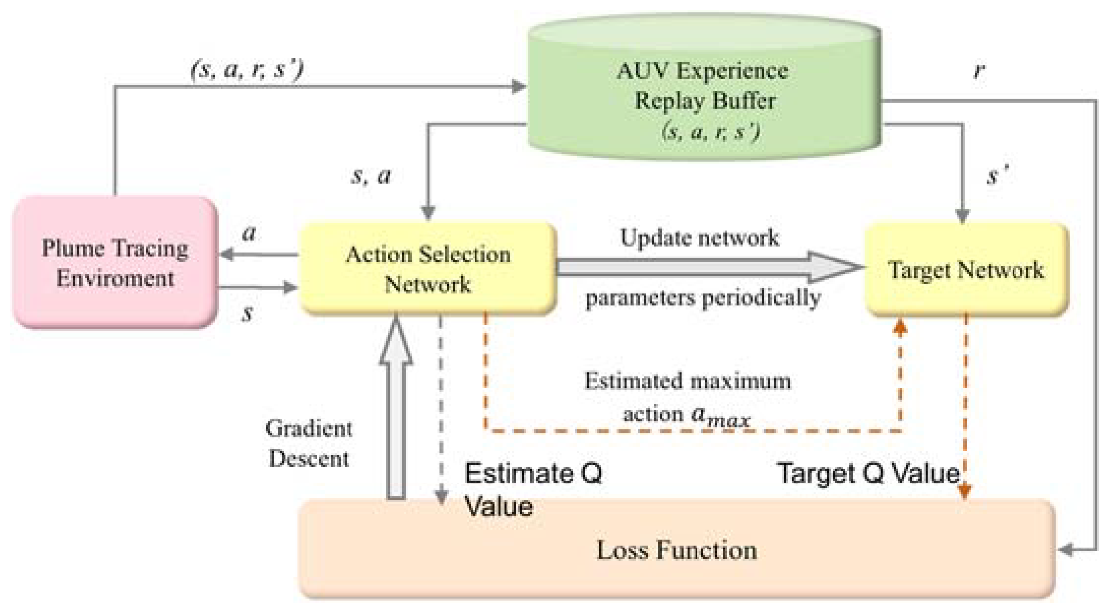
Figure 3 shows a diagram of the DDQN algorithm for AUV path planning for plume tracing. The algorithm starts from initialization of the action selection network and the target network, and the experience replay buffer as well. In each iteration, the Q-values of state–action pairs are updated. The corresponding actions are selected using the ϵ−greedy approach. The current state, the action taken, the reward received, and the next state constitute one experience. Experiences are saved in the AUV experience replay buffer, where training samples are extracted for Q-value estimation. The predicted Q-value is calculated by the action selection network using the current state and action as the input, while the target value is calculated by the target network using the next state and the action associated with the maximal predicted Q-value obtained from the action selection network. The loss is calculated using the predicted Q-values and the target values for the sampled experiences. The weights of the action selection network are updated via backpropagation. The target network’s weights are periodically updated to match the action selection network’s weights.

4. Numerical Simulation and Results

4.1. Numerical Simulation Setup

To demonstrate the feasibility of the model-free reinforcement learning approach to plume tracing problems, a series of numerical experiments were conducted. The numerical experiments are designed based on current AUVs’ endurance, which ranges from hours to days, and even months [8]. In the numerical experiments, the distribution of plume concentration is designed as nearly the worst case, in which the distance between the deployment location and the plume source is comparable to the AUV’s survey range. The parameters used in the numerical experiments are listed in Table 1.
In the numerical experiments, the AUV is deployed at the left lower corner of the survey region and starts exploring the environment after deployment. It takes measurement and makes decisions on the next waypoint at a constant time interval. The restriction on the AUV’s survey endurance turns into an upper bound on the total time steps in the experiments. The AUV is supposed to have eight possible actions at each state. It can move in north, south, east, west, northeast, northwest, southeast, and southwest directions. Two plume models are used to evaluate the performance of the presented approach in the cases of steady and transient plumes.
For our numerical simulation employing DRL algorithms, we utilized a computational setup comprising an Intel Core i5-12500H processor with 16 GB RAM and an NVIDIA RTX 3060 GPU. The operating system deployed was Ubuntu 20.04.4 LTS. We conducted our experiments using Python 3.7, with PyTorch 1.11.0 as the deep learning framework. Our models were trained on the OpenAI Gym environment, utilizing a convolutional neural network architecture with a learning rate of 0.001.

4.2. Plume Models

The subsurface oil plumes resulted from an accidental blowout are distinct from natural hydrocarbon seep plumes. Natural seep plumes are usually continuous releases from underwater sources, while the plumes formed in an accident are caused by instantaneous ejection of oil into the water. Gaussian models are frequently used to predict the behavior and impact of pollutants in marine environments [36]. In this work, a 2D Gaussian puff model [37] is used to simulate the evolution of transient plumes.
According to the Gaussian puff model, plume concentrations can be expressed as the solution of the transport equation as:
c x , y , t = M 4 π t D x D y exp 1 4 x v c x t 2 D x t + y v c y t 2 D y t
where M is the total mass of hydrocarbon contained in the puff, v c x , v c y T is the vector of ocean current velocity, and D x and D y are diffusion coefficients. The initial condition for this solution is the peak with infinite concentration at position (0,0) and zero boundary condition at infinity.
The subsurface oil plumes often have complex structures and are characterized by many local extrema [38]. These plumes may also be discontinuous and patchy in a turbulent marine environment with the application of dispersants. In this work, we use the Ackley function to represent a steady plume with multiple local minima and one global maximum. It can be expressed as:
c x , y = a exp b x 2 + y 2 2 exp c o s k x + c o s k y 2 + a + e x p 1
where a, b, and k are formula coefficients.

4.3. Steady Plume Tracing

In this section, we use the Ackley function to simulate a steady subsurface plume. It is a static test function commonly used in optimization and representative of substance diffusing away from a potent source [33]. Figure 4 shows a contour plot of the Ackley function.
Autonomous surveying within an unknown region with multiple local minima and maxima is not a trivial problem. AUVs may be trapped into local extrema and fail to find the plume source. We consider three survey strategies with different initial sampling conditions. The first strategy is to have 30 episodes of random walk, the second is to have 30 episodes of uniform sampling over the survey region, while the last one does not involve any initial sampling. The asymptotic performances of the three learning processes are indicated in Figure 5 and Figure 6.
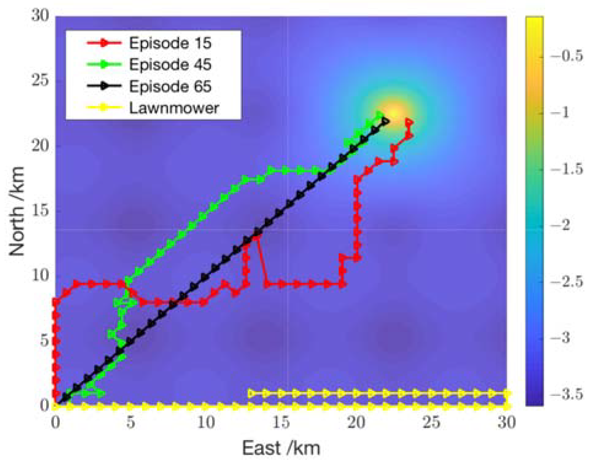
The results show that, in the perspective of asymptotic performance, the adaptive path planning approach performs comparably under the three survey strategies. The learning processes are equivalently efficient. The initial uniform sampling strategy may outperform the other two on stability during convergence. It is also observed that there is not much deviation in the interim performance. Estimates are also made of the earliest episode when the plume source is detected and the number of successful attempts within the first one hundred episodes. The results are shown in Table 2. Comparison between the three strategies shows that the third survey strategy, i.e., direct learning without initial sampling, may be the optimal strategy, because initial sampling induces additional costs. Figure 7 shows an improvement on the survey path in the learning process when the AUV starts learning without any experience. It can be observed that as the learning process proceeds, the continuous interaction with the environment enables the AUV to autonomously follow a shorter path toward the plume source.

4.4. Transient Plume Tracing

In the transient case, the plume in the region of interest is generated by a Gaussian pull model. It is assumed that the emission source is an instantaneous source located within the survey region and the ocean current is represented by a uniform flow field. The diffusion coefficient in the horizontal plane is adopted as of the order of 1 m2/s [39]. The parameters used in the simulation are listed in Table 3.
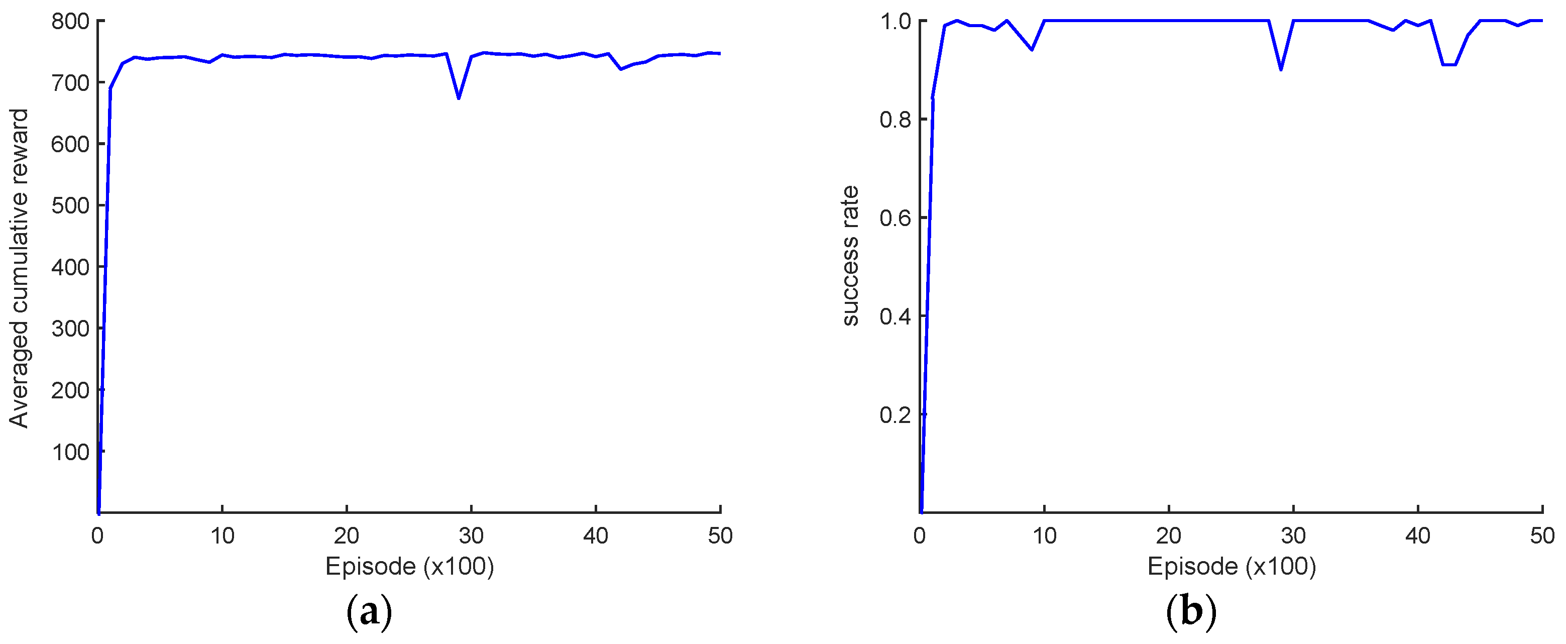
The results from the case of steady plume tracing show that initial sampling may not be as beneficial as we believed. In transient plume tracing, we switched the survey strategy and let the AUV learn from the scratch. A fast convergence is observed in Figure 8, indicating an efficient learning process. It shows that the AUV can learn an optimal path to the plume source after around two hundred attempts. It may seem rather time-consuming at first glance, but an inspiring clue is found when we take a closer look into the first one hundred attempts. Repetitive runs show that the AUV arrives at a proximity to the plume source within about 20 surveys. Figure 9 illustrates one instance of AUV adaptive survey process. It presents the first successful attempt to locate the plume source in one run. The source locating process is illustrated by time evolution.

4.5. Learning Performance

Learning performance is crucial for applying DRL approaches to plume source tracing problems. Using DRL approaches, AUVs can learn from interactions with ocean environments and gain knowledge of the plume under investigation. The learning performance of DRL algorithms is closely related to survey efficiency.
In this section, comparative investigation is conducted between the developed DDQN algorithm and the Proximal Policy Optimization (PPO) algorithm. PPO is a widely employed strategy optimization algorithm in the realm of reinforcement learning [40]. It is a policy gradient-based approach, which is different to value function-based algorithms like DDQN. The PPO framework is based on actor–critic architecture. The actor network is responsible for generating actions, while the critic network evaluates the performance of the agent. The learning performance of the DDQN and PPO algorithms on the plume tracing examples are compared in Table 4. These results are obtained using the same reward structure.
In Table 4, the high success rate of reaching the global extreme value in the two plume structures indicates that both DDQN and PPO can be used to find a survey path to the plume source. It is also indicated that the DDQN algorithm outperforms the PPO algorithm in the learning efficiency. The PPO algorithm converges much slower than the DDQN algorithm, roughly in two orders of magnitude. Similar results can be inferred from the data of the first successful episode. It is observed that the first successful episode obtained by the DDQN algorithm also appears earlier in two orders of magnitude than the PPO algorithm.
The difference in the algorithm performance consists in their learning mechanism. In the DDQN algorithm, the action value is evaluated through the target network and the optimal action is selected using the action selection network. While in the PPO algorithm, the policy function is directly optimized. The policy is represented by a probability distribution over possible actions at the current state. This requires a large amount of training data to achieve good performance. Therefore, from a cost-effectiveness point of view, the DDQN algorithm would be more suitable for plume source tracing problems in engineering practice.

4.6. Comparison with Lawnmower Approach

Lawnmower pattern is a canonical survey approach commonly used in engineering practice to achieve full coverage over a studied region. It is used in oceanographic observation based on previous knowledge on oceanic phenomena, and adequate representation of the studied region can often be obtained [41]. However, it may not be a good option for plume source tracing using AUVs because prior knowledge of the plume concentration is not available, and due to energy limitation, AUVs may not be able to complete a full coverage survey, especially over a large survey region.
This section presents a comparison between the proposed adaptive approach and the lawnmower approach. In both cases of the steady and transit plumes, survey paths generated by the adaptive approach and the lawnmower approach are presented in Figure 7 and Figure 9, respectively. These results indicate that the adaptive path planning approach eventually provides a feasible solution to the plume source tracing problem, but it may take much time to learn from the interactions with the environment. As indicated in the results presented in Section 4.3 and Section 4.4, about 50 episodes are required to detect the source of the steady plume represented by the Ackley function, and 20 episodes are needed for the Gaussian transit plume. In the case of the lawnmower survey pattern, we suppose a survey range of 60 km and a 1 km distance between the track lines for each operation, corresponding to 60 time steps in the numerical simulation. The individual operation time can then be obtained by a simple calculation as 33 h and 20 min. A total of 15 successive operations would be required to achieve full coverage over the survey region. When only one AUV is utilized, the total survey time is an accumulation of the duration of every individual operation. The comparison on the total survey time required by the adaptive approach and the lawnmower approach is presented in Figure 10. It is apparent that the lawnmower survey pattern would be a better strategy when only one AUV is available, especially when the plume structure is complex.
For large-scale or long-range surveys, as indicated in our presented example considering the capability of the AUV and the requirement of the survey task, it would be more time-effective to use multiple AUVs. Take the steady plume tracing problem demonstrated in Section 4.3 as an example. When the lawnmower survey pattern is adopted, AUVs operate in a relay mode and the total survey time is estimated as 500 h, while in the case of the adaptive survey approach, the total survey time is calculated based on the estimate of the first successful survey, as presented in Table 1. Here, for simple calculation, we suppose 50 individual surveys are needed and each survey is also restricted to a duration of 33 h and 20 min. Because multiple AUVs can operate in a parallel mode, the survey efficiency increases as the number of AUVs simultaneously used increases. It can be safely concluded from the comparison in Figure 10 that the adaptive survey approach is more efficient than the lawnmower approach when more than three AUVs operate in parallel.

5. Experiment with AGV

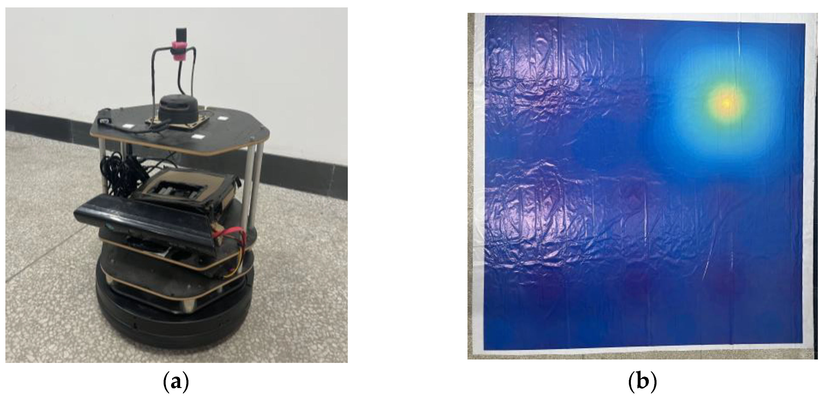
This section presents the experiment used to demonstrate the feasibility of using the adaptive path planning algorithm for autonomous robot navigation to locate the global extreme in a static environment. In the experiment, a TurtleBot 2 robot with Kobuki base, as shown in Figure 11, was deployed to locate the extreme point on a 3 m × 3 m map. The map was printed with the same contour plot of the Ackley environment feature as presented in the numerical simulation in Section 4.4. The robot was equipped with a Microsoft Kinect V1 Xbox 360 (Redmond, WA, USA), which relayed real-time visual data to a remote computer. This computer, running Ubuntu 14.04 and equipped with an AMD Ryzen 7 5800H processor (Surry Hills, NSW, Australia), 16 GB of RAM, and an NVIDIA RTX 3060 GPU, processed the data using the developed DDQN algorithm implemented in PyTorch 1.11.0. The TurtleBot 2 robot and the remote computer were configured to set up communications on the same network. The IP address was used to established the ROS environment variable for communication.
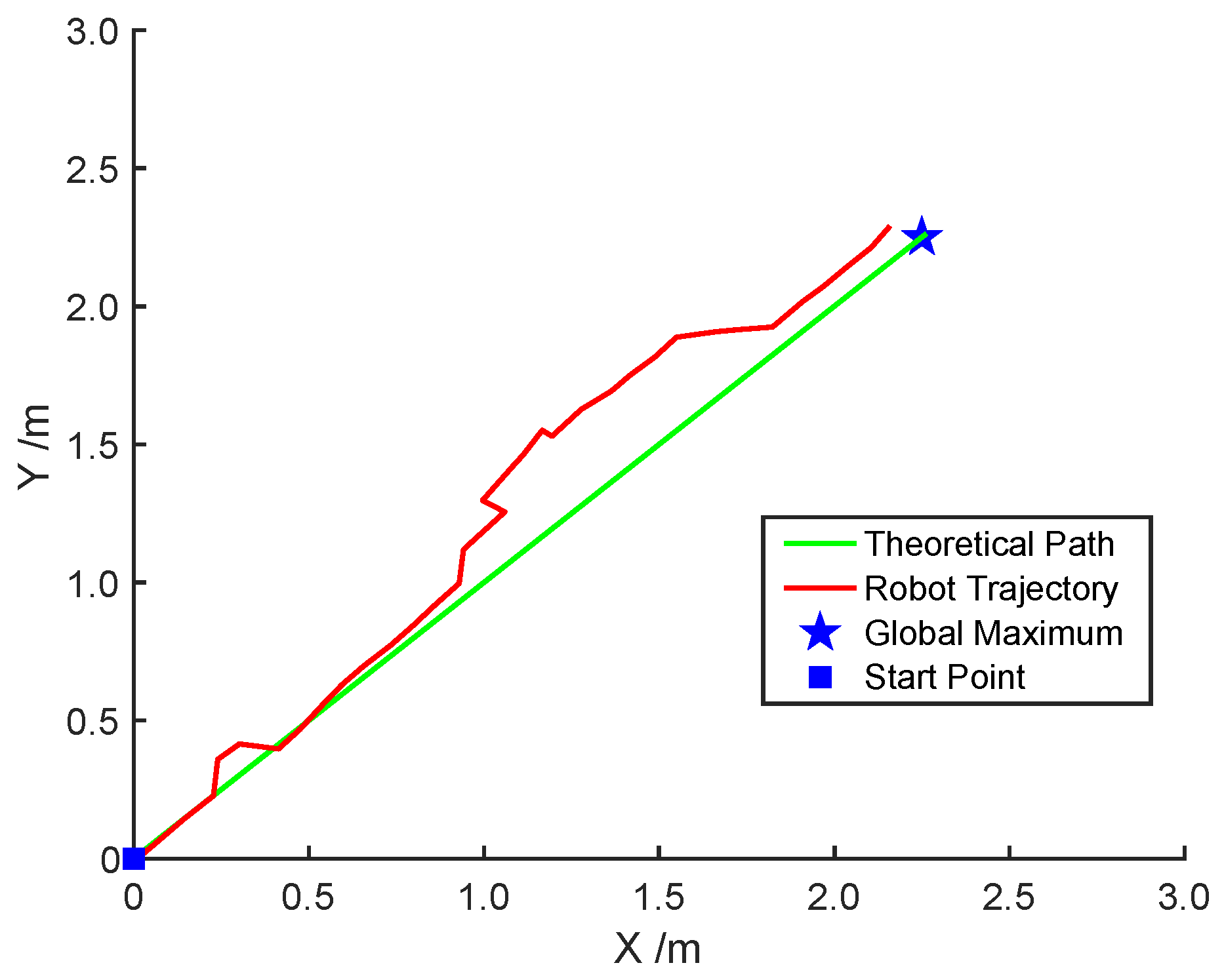
In the experiment, the robot moved with a step size of 100 mm, and the maximum number of steps was set as 60. The global extreme locating task is believed to be successfully completed if within 60 steps, the robot arrives at a location that is less than 100 mm from the destination; otherwise, it fails. Figure 12 shows the autonomous navigation process using the proposed adaptive path planning approach, and Table 5 lists the experimental results. It took the robot 36 steps to arrive to the proximity of the global extreme. The actual robot trajectory and the theoretical optimal path are demonstrated in Figure 13. The experimental outcomes showed that the robot could autonomously move to the proximity of the global maximum using the proposed adaptive path planning approach. The distance between the robot’s final location and the goal is around 94 mm. The deviation between the robot’s trajectory and the theoretical path may be a result of actuation error and sensor uncertainty.

6. Conclusions

In this paper, we present an adaptive path planning approach for AUVs to autonomously locate the subsurface plume source. The plume tracing problem is analogous to unknown environment exploration. The similarity consists in the lack of prior knowledge on the interest of concern. This presented approach is developed in the reinforcement learning paradigm, using a model-free DDQN algorithm. AUVs could learn from interactions with marine environments and acquire the mapping from a state to an optimal maneuver. Although the application of reinforcement learning approaches in real-world applications may sometimes seem impractical because it usually takes considerable time for the agent to learn the optimal strategy, it is indicated in our preliminary results that this learning paradigm may be appropriate for the plume tracing problem because the goal is to locate the source, which may be accomplished before the training process is completed. It is also indicated that adaptive path planning approach developed in the deep reinforcement learning framework can be more efficient than the conventional lawnmower survey pattern in large-scale exploration when multiple AUVs operate in a parallel mode.

7. Future Work

AUVs are well suited for unknown environment exploration. They could operate autonomously in remote areas that might be hostile or dangerous to human beings. Implementation of artificial intelligent algorithms could enable AUVs to make intelligent decisions and incorporation of the adverse conditions into these algorithms could eventually achieve an increase in the degree of autonomy. This work presents an adaptive path planning approach for plume tracing problems. To apply this approach in engineering practice, the following aspects will be investigated in the future work.
  • Dynamics of ocean currents. Ocean currents are the major environmental factors that affect AUVs’ motion and path planning. In this work, we consider a simplified case of uniform flow field. The dynamics of ocean currents will be included into the algorithm by sophisticated modeling or oceanographic data for more accurate estimation.
  • Obstacle avoidance. Underwater obstacles such as subsea terrain features and man-made structures can pose navigation hazards to AUVs. Strategies will be designed for collision avoidance in the reinforcement learning framework.
  • Sensor and actuation errors. Variations in water density, temperature, and salinity can affect acoustic communication and influence the performance of sensors for navigation. In this work, we model the AUV decision-making processes as MDPs. The MDP model will be replaced by Partially Observable Markov Decision Process (POMDP) to represent influence of these uncertainties.
  • AUV field trials. Field trials play an important role in path planning algorithm testing. The algorithm performance needs to be evaluated and the models used within can then be improved using measurement and data from underwater experiments.

Author Contributions

Conceptualization, Z.W. and F.L.; methodology, Z.W. and S.W.; software, X.S. and Z.B.; validation, X.S. and S.W.; formal analysis, Z.W. and X.S.; investigation, F.L.; resources, Z.W.; writing—original draft preparation, Z.W., X.S. and S.W.; writing—review and editing, S.W.; visualization, S.W. and X.S.; project administration, F.L. All authors have read and agreed to the published version of the manuscript.

Funding

This research was funded by the National Natural Science Foundation of China, grant number 52375025. The APC was funded by MDPI Robotics.

Data Availability Statement

The datasets generated and supporting the findings of this article are obtainable from the corresponding author upon reasonable request.

Acknowledgments

The authors would like to thank the editors for their recommendation. We would also like to thank the reviewers for their comments and constructive suggestions that help us improve the quality of our manuscript.

Conflicts of Interest

The authors declare no conflicts of interest. The funders had no role in the design of the study; in the collection, analyses, or interpretation of data; in the writing of the manuscript; or in the decision to publish the results.

References

  1. Beyer, J.; Trannum, H.C.; Bakke, T.; Hodson, P.V.; Collier, T.K. Environmental effects of the Deepwater Horizon oil spill: A review. Mar. Pollut. Bull. 2016, 110, 28–51. [Google Scholar] [CrossRef]
  2. Westerholm, D.A.; Rauch, S.D., III. Deepwater Horizon Oil Spill: Final Programmatic Damage Assessment and Restoration Plan and Final Programmatic Environmental Impact Statement. Deep. Horiz. Nat. Resour. Damage Assess. Trustees 2016. [Google Scholar]
  3. Zhang, Y.; McEwen, R.S.; Ryan, J.P.; Bellingham, J.G.; Thomas, H.; Thompson, C.H.; Rienecker, E. A peak-capture algorithm used on an autonomous underwater vehicle in the 2010 Gulf of Mexico oil spill response scientific survey. J. Field Robot. 2011, 28, 484–496. [Google Scholar] [CrossRef]
  4. Kujawinski, E.B.; Soule, M.C.K.; Valentine, D.L.; Boysen, A.K.; Longnecker, K.; Redmond, M.C. Fate of Dispersants Associated with the Deepwater Horizon Oil Spill. Environ. Sci. Technol. 2011, 45, 1298–1306. [Google Scholar] [CrossRef] [PubMed]
  5. Jones, C.E.; Dagestad, K.; Breivik, Ø.; Holt, B.; Röhrs, J.; Christensen, K.H.; Espeseth, M.; Brekke, C.; Skrunes, S. Measurement and modeling of oil slick transport. J. Geophys. Res. Ocean. 2016, 121, 7759–7775. [Google Scholar] [CrossRef]
  6. Hwang, J.; Bose, N.; Nguyen, H.D.; Williams, G. Acoustic Search and Detection of Oil Plumes Using an Autonomous Underwater Vehicle. J. Mar. Sci. Eng. 2020, 8, 618. [Google Scholar] [CrossRef]
  7. Camilli, R.; Reddy, C.M.; Yoerger, D.R.; Van Mooy, B.A.S.; Jakuba, M.V.; Kinsey, J.C.; McIntyre, C.P.; Sylva, S.P.; Maloney, J.V. Tracking Hydrocarbon Plume Transport and Biodegradation at Deepwater Horizon. Science 2010, 330, 201–204. [Google Scholar] [CrossRef]
  8. Wynn, R.B.; Huvenne, V.A.I.; Le Bas, T.P.; Murton, B.J.; Connelly, D.P.; Bett, B.J.; Ruhl, H.A.; Morris, K.J.; Peakall, J.; Parsons, D.R.; et al. Autonomous Underwater Vehicles (AUVs): Their past, present and future contributions to the advancement of marine geoscience. Mar. Geol. 2014, 352, 451–468. [Google Scholar] [CrossRef]
  9. Reddy, C.M.; Arey, J.S.; Seewald, J.S.; Sylva, S.P.; Lemkau, K.L.; Nelson, R.K.; Carmichael, C.A.; McIntyre, C.P.; Fenwick, J.; Ventura, G.T.; et al. Composition and fate of gas and oil released to the water column during the Deepwater Horizon oil spill. Proc. Natl. Acad. Sci. USA 2012, 109, 20229–20234. [Google Scholar] [CrossRef]
  10. DiPinto, L.; Forth, H.; Holmes, J.; Kukulya, A.; Conmy, R.; Garcia, O. Three-Dimensional Mapping of Dissolved Hydrocarbons and Oil Droplets Using a REMUS-600 Autonomous Underwater Vehicle. In Report to Bureau of Safety and Environmental Enforcement; BSEE: New Orleans, LA, USA, 2019. [Google Scholar]
  11. Hwang, J.; Bose, N.; Millar, G.; Gillard, A.B.; Nguyen, H.D.; Williams, G. Enhancement of AUV Autonomy Using Backseat Driver Control Architecture. Int. J. Mech. Eng. Robot. Res. 2021, 10, 292–300. [Google Scholar] [CrossRef]
  12. Gomez-Ibanez, D.; Kukulya, A.L.; Belani, A.; Conmy, R.N.; Sundaravadivelu, D.; DiPinto, L. Autonomous Water Sampler for Oil Spill Response. J. Mar. Sci. Eng. 2022, 10, 526. [Google Scholar] [CrossRef]
  13. Berg, H.C. Bacterial microprocessing. Cold Spring Harb. Symp. Quant. Biol. 1990, 55, 539–545. [Google Scholar] [CrossRef] [PubMed]
  14. Petillo, S.; Schmidt, H.R. Autonomous and Adaptive Underwater Plume Detection and Tracking with AUVs: Concepts, Methods, and Available Technology. IFAC Proc. Vol. 2016, 45, 232–237. [Google Scholar] [CrossRef]
  15. Farrell, J.A.; Pang, S.; Li, W. Chemical plume tracing via an autonomous underwater vehicle. IEEE J. Ocean. Eng. 2005, 30, 428–442. [Google Scholar] [CrossRef]
  16. Li, W.; Farrell, J.; Pang, S.; Arrieta, R. Moth-inspired chemical plume tracing on an autonomous underwater vehicle. IEEE Trans. Robot. 2006, 22, 292–307. [Google Scholar] [CrossRef]
  17. Grasso, F.W.; Atema, J. Integration of Flow and Chemical Sensing for Guidance of Autonomous Marine Robots in Turbulent Flows. Environ. Fluid Mech. 2002, 2, 95–114. [Google Scholar] [CrossRef]
  18. Hu, H.; Song, S.; Chen, C.L.P. Plume Tracing via Model-Free Reinforcement Learning Method. IEEE Trans. Neural Netw. Learn. Syst. 2019, 30, 2515–2527. [Google Scholar] [CrossRef]
  19. Marques, L.; Nunes, U.; de Almeida, A.T. Particle swarm-based olfactory guided search. Auton Robot. 2006, 20, 277–287. [Google Scholar] [CrossRef]
  20. Yang, B.; Ding, Y.; Jin, Y.; Hao, K. Self-organized swarm robot for target search and trapping inspired by bacterial chemotaxis. Robot. Auton. Syst. 2015, 72, 83–92. [Google Scholar] [CrossRef]
  21. Marjovi, A.; Marques, L. Optimal Swarm Formation for Odor Plume Finding. IEEE Trans. Cybern. 2014, 44, 2302–2315. [Google Scholar] [CrossRef]
  22. Sampathkumar, A.; Dugaev, D.; Song, A.; Hu, F.; Peng, Z.; Zhang, F. Plume tracing simulations using multiple autonomous underwater vehicles. In Proceedings of the 16th International Conference on Underwater Networks & Systems, Association for Computing Machinery, Boston, MA, USA, 14–16 November 2022. [Google Scholar]
  23. Smith, R.N.; Chao, Y.; Li, P.P.; Caron, D.A.; Jones, B.H.; Sukhatme, G.S. Planning and implementing trajectories for autonomous underwater vehicles to track evolving ocean processes based on predictions from a regional ocean model. Int. J. Robot. Res. 2010, 29, 1475–1497. [Google Scholar] [CrossRef]
  24. Li, R.; Wu, H. Multi-robot plume source localization by distributed quantum-inspired guidance with formation behavior. IEEE Trans. Intell. Transp. Syst. 2023, 24, 11889–11904. [Google Scholar] [CrossRef]
  25. Zhou, Y.; Wang, T.; Lei, X.; Peng, X. Collective behavior of self-propelled particles with heterogeneity in both dynamics and delays. Chaos Solitons Fractals 2024, 180, 114596. [Google Scholar] [CrossRef]
  26. Wang, T.; Peng, X.; Wang, T.; Liu, T.; Xu, D. Automated design of action advising trigger conditions for multiagent reinforcement learning: A genetic programming-based approach. Swarm Evol. Comput. 2024, 85, 101475. [Google Scholar] [CrossRef]
  27. Pang, S.; Farrell, J.A. Chemical Plume Source Localization. IEEE Trans. Syst. Man Cybern. Part B (Cybern.) 2006, 36, 1068–1080. [Google Scholar] [CrossRef]
  28. Jiu, H.-F.; Chen, Y.; Deng, W.; Pang, S. Underwater chemical plume tracing based on partially observable Markov decision process. Int. J. Adv. Robot. Syst. 2019, 16. [Google Scholar] [CrossRef]
  29. Marchant, R.; Ramos, F. Bayesian optimisation for Intelligent Environmental Monitoring. In Proceedings of the 2012 IEEE/RSJ International Conference on Intelligent Robots and Systems, Vilamoura-Algarve, Portugal, 7–12 October 2012. [Google Scholar]
  30. Wang, L.; Pang, S. Autonomous underwater vehicle based chemical plume tracing via deep reinforcement learning methods. J. Mar. Sci. Eng. 2023, 11, 366. [Google Scholar] [CrossRef]
  31. Bao, Z.; Li, Y.; Shao, X.; Wu, Z.; Li, Q. Adaptive path planning for plume detection with an underwater glider. In Proceedings of the IFToMM World Congress on Mechanism and Machine Science, Tokyo, Japan, 5–10 November 2023. [Google Scholar]
  32. Zhang, Y.; Hobson, B.W.; Kieft, B.; Godin, M.A.; Ravens, T.; Ulmgren, M. Adaptive Zigzag Mapping of a Patchy Field by a Long-Range Autonomous Underwater Vehicle. IEEE J. Ocean. Eng. 2024, 49, 403–415. [Google Scholar] [CrossRef]
  33. Blanchard, A.; Sapsis, T. Informative path planning for anomaly detection in environment exploration and monitoring. Ocean. Eng. 2022, 243, 110242. [Google Scholar] [CrossRef]
  34. Bracco, A.; Paris, C.B.; Esbaugh, A.J.; Frasier, K.; Joye, S.B.; Liu, G.; Polzin, K.L.; Vaz, A.C. Transport, Fate and Impacts of the Deep Plume of Petroleum Hydrocarbons Formed During the Macondo Blowout. Front. Mar. Sci. 2020, 7, 542147. [Google Scholar] [CrossRef]
  35. Su, F.; Fan, R.; Yan, F.; Meadows, M.; Lyne, V.; Hu, P.; Song, X.; Zhang, T.; Liu, Z.; Zhou, C.; et al. Widespread global disparities between modelled and observed mid-depth ocean currents. Nat. Commun. 2023, 14, 1–9. [Google Scholar] [CrossRef]
  36. Lewis, T.; Bhaganagar, K. A comprehensive review of plume source detection using unmanned vehicles for environmental sensing. Sci. Total Environ. 2021, 762, 144029. [Google Scholar] [CrossRef]
  37. Holzbecher, E. Environmental Modeling Using MATLAB; Springer: Berlin/Heidelberg, Germany, 2012; pp. 303–316. [Google Scholar]
  38. Naeem, W.; Sutton, R.; Chudley, J. Chemical Plume Tracing and Odour Source Localisation by Autonomous Vehicles. J. Navig. 2007, 60, 173–190. [Google Scholar] [CrossRef]
  39. Paris, C.B.; Le Hénaff, M.; Aman, Z.M.; Subramaniam, A.; Helgers, J.; Wang, D.-P.; Kourafalou, V.H.; Srinivasan, A. Evolution of the Macondo Well Blowout: Simulating the Effects of the Circulation and Synthetic Dispersants on the Subsea Oil Transport. Environ. Sci. Technol. 2012, 46, 13293–13302. [Google Scholar] [CrossRef] [PubMed]
  40. Boudlal, A.; Khafaji, A.; Elabbadi, J. Entropy adjustment by interpolation for exploration in Proximal Policy Optimization (PPO). Eng. Appl. Artif. Intell. 2024, 113, 108401. [Google Scholar] [CrossRef]
  41. Foster, S.D.; Hosack, G.R.; Hill, N.A.; Barrett, N.S.; Lucieer, V.L. Choosing between strategies for designing surveys: Autonomous underwater vehicles. Methods Ecol. Evol. 2014, 5, 287–297. [Google Scholar]
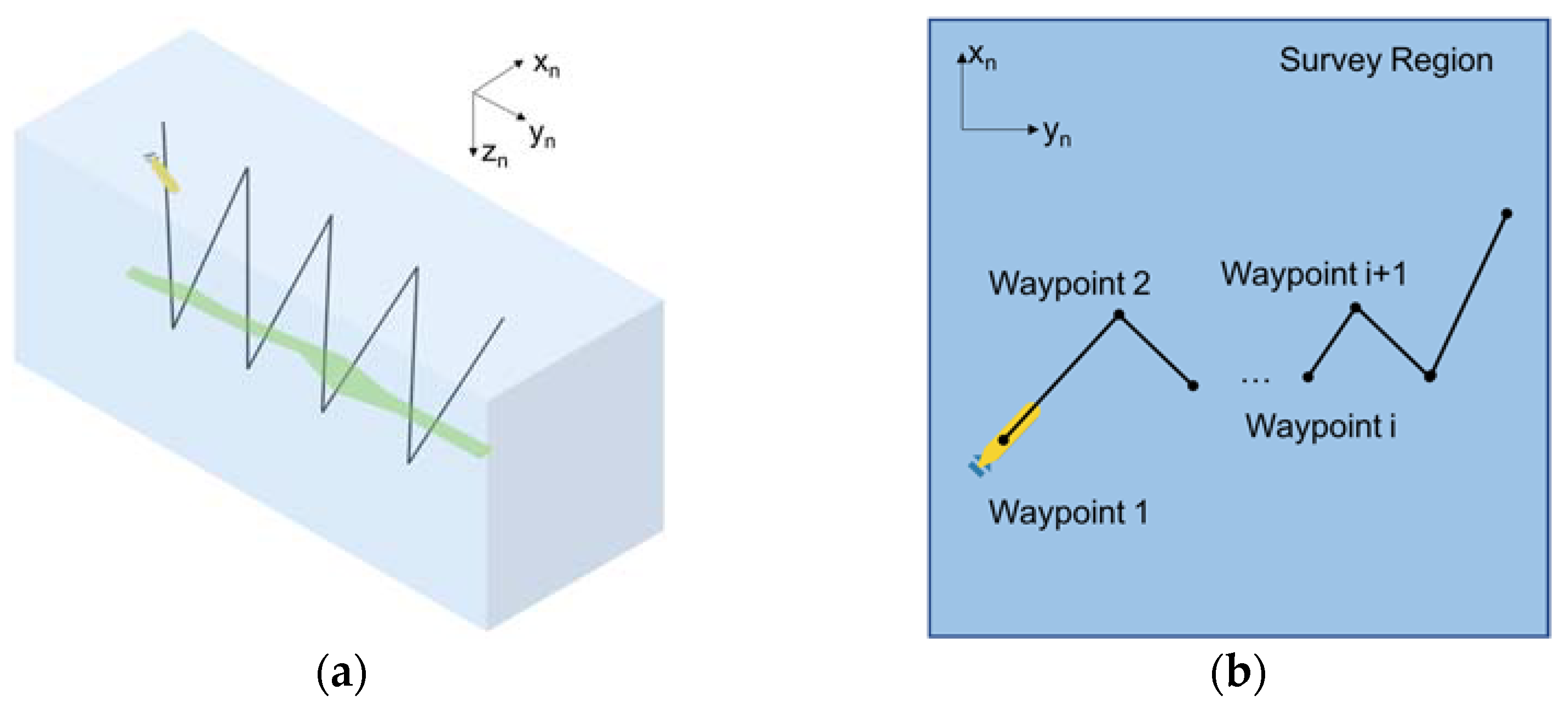
Figure 1. Schematics of AUV plume tracing phases: (a) Phase I: Sawtooth survey in the vertical plane; (b) Phase II: Plume characterization in the horizontal plane.
Robotics 13 00132 g001
Figure 2. AUV kinematic model in the NED system, where {xb, yb} denotes the body-fixed reference frame, α indicates the direction of the ocean current, and β denotes the angular difference between the NED system and the body-fixed reference frame.
Robotics 13 00132 g002
Figure 3. DDQN algorithm for AUV path planning for plume tracing, where s and s′ denote the current and the next states, respectively, a denotes the action taken, amax denotes the action corresponding to the maximal Q-value output from the action selection network, r denotes the immediate reward received after the action is executed, and {s,a,r,s′} denotes the experiences saved in the AUV experience replay buffer.
Robotics 13 00132 g003
Figure 4. Contour plot of the Ackley function as a steady plume. The picture is generated using Equation (5) with the coefficients a = −36, b = 2.2, and k = π.
Robotics 13 00132 g004
Figure 5. Asymptotic performance of the DDQN algorithm in the averaged cumulative reward: (a) survey strategy with 30 initial random sampling episodes; (b) survey strategy with 30 initial uniform sampling episodes; (c) survey strategy without initial sampling.
Robotics 13 00132 g005
Figure 6. Asymptotic performance of the DDQN algorithm in the success rate: (a) survey strategy with 30 initial random sampling episodes; (b) survey strategy with 30 initial uniform sampling episodes; (c) survey strategy without initial sampling.
Robotics 13 00132 g006
Figure 7. Evolution of the adaptive survey path w/o initial sampling. The AUV starts from the left lower corner. The red, green, and black lines are survey paths generated by the proposed approach in learning process, and the yellow line is the lawnmower path.
Robotics 13 00132 g007
Figure 8. Asymptotic performance of the DDQN algorithm in transient plume tracing: (a) averaged cumulative reward, indicating the average over every one hundred episodes; (b) success rate, indicating the rate of successfully arriving at the plume source over every one hundred episodes.
Robotics 13 00132 g008
Figure 9. Transient plume tracing using adaptive path planning and lawnmower survey pattern: (a) Stage 1: 10 time steps (~5.5 h); (b) Stage 2: 20 time steps (~11 h); (c) Stage 3: 30 time steps (~16.5 h); (d) Stage 4: 42 time steps (~23 h).
Robotics 13 00132 g009aRobotics 13 00132 g009b
Figure 10. Total survey time needed with different number of AUVs used in the steady plume source tracing problem. The time for individual operation in the lawnmower approach and the adaptive approach is setup as 60 time steps in the numerical simulation or 33 h and 20 min according to the preset vehicle endurance. Note that when one AUV is utilized, the battery charging time is ignored in the calculation.
Robotics 13 00132 g010
Figure 11. TurtleBot 2 and the map used in the experiment: (a) TurtleBot 2; (b) the map printed with a contour plot of the Ackley function with the coefficients a = −36, b = 2.2, and k = π. The global maximum is indicated with a color of bright yellow.
Robotics 13 00132 g011
Figure 12. Snapshots of TurtleBot 2 robot autonomous navigation in the static Ackley environment.
Robotics 13 00132 g012
Figure 13. Robot trajectory in the static Ackley environment.
Robotics 13 00132 g013
Table 1. Numerical experiment setup.
ParameterValue
Survey region 30 km × 30 km
AUV survey endurance36 h
Total time step limit per survey60
AUV speed0.5 m/s
Time step length 2000 s
Table 2. Performance comparison between three initial sampling strategies *.
Initial Sampling StrategyEarliest
Successful Episode
Number of Successful Episodes
within the First 100 Attempts
Random 55th21
Uniform 59th19
w/o53rd23
* Results are averaged over one hundred runs.
Table 3. Parameters in the case of transient plume tracing.
ParameterValueNote
Ocean current velocity0.1 m/sin the positive horizontal direction
Diffusion coefficient1 m2/shorizontal
Table 4. Performance of DDQN and PPO on the steady and transient plume tracing problems *.
Steady PlumeTransit Plume
DDQNPPODDQNPPO
Success rate100%100%100%100%
First successful episode~50th3000th~20th1800th
Convergence speed~300 eps~2.8 × 10⁴ eps~400 eps~3.7 × 10⁴ eps
* Results are averaged over one hundred runs.
Table 5. Results of TurtleBot 2 robot experiment.
ParameterPreset ValueExperimental ResultQualified (Yes/No)
Number of steps6036Yes
Distance to the goal (mm)100 94 Yes
Disclaimer/Publisher’s Note: The statements, opinions and data contained in all publications are solely those of the individual author(s) and contributor(s) and not of MDPI and/or the editor(s). MDPI and/or the editor(s) disclaim responsibility for any injury to people or property resulting from any ideas, methods, instructions or products referred to in the content.