Fixed-Wing UAV Pose Estimation Using a Self-Organizing Map and Deep Learning

Abstract

In many Unmanned Aerial Vehicle (UAV) operations, accurately estimating the UAV’s position and orientation over time is crucial for controlling its trajectory. This is especially important when considering the landing maneuver, where a ground-based camera system can estimate the UAV’s 3D position and orientation. A Red, Green, and Blue (RGB) ground-based monocular approach can be used for this purpose, allowing for more complex algorithms and higher processing power. The proposed method uses a hybrid Artificial Neural Network (ANN) model, incorporating a Kohonen Neural Network (KNN) or Self-Organizing Map (SOM) to identify feature points representing a cluster obtained from a binary image containing the UAV. A Deep Neural Network (DNN) architecture is then used to estimate the actual UAV pose based on a single frame, including translation and orientation. Utilizing the UAV Computer-Aided Design (CAD) model, the network structure can be easily trained using a synthetic dataset, and then fine-tuning can be done to perform transfer learning to deal with real data. The experimental results demonstrate that the system achieves high accuracy, characterized by low errors in UAV pose estimation. This implementation paves the way for automating operational tasks like autonomous landing, which is especially hazardous and prone to failure.

1. Introduction

The research on Unmanned Aerial Vehicles (UAVs) are very popular nowadays [1], being used for several applications, such as surveillance [2,3], Search And Rescue (SAR) [4,5], remote sensing [6,7], military Intelligence, Surveillance and Reconnaissance (ISR) operations [8,9], sea pollution monitoring and control [10,11], among many others. Performing UAV autonomous control is essential since it can decrease human intervention [12,13], increasing the system’s operational capabilities and reliability [14]. In typical UAV operations, the most dangerous stages are usually the take-off and landing [15,16], and the automation of these stages is essential to increase the safety of personnel and material, thus increasing the overall system reliability.

A rotary-wing UAV, due to its operational capabilities, can easily perform Vertical Take-Off and Landing (VTOL) [17]. Still, the same thing does not usually happen in the fixed-wing UAV case [18,19]. However, some fixed-wing currently present VTOL capability [20,21]. They are only suitable for certain operations where the platform may be stationary for a specific time period, and the landing’s site weather conditions allow a successful landing [22]. Using a ground-based Red, Green, and Blue (RGB) vision system to estimate the pose of a fixed-wing UAV can help adjust its trajectory during flight and perform guidance during a landing maneuver [23]. In real-life operations, all the possible incorporation of data in the control loop [12] should be considered since it will facilitate the operator’s operational procedures, decreasing the accident probability.

The standard UAV mission profile commonly consists of three stages, as illustrated in Figure 1. It typically includes a climb, a mission envelope, and the descent to perform landing, usually following a well-defined trajectory state machine [24]. In a typical landing trajectory state machine, the UAV performs loiters around the landing site’s predefined position until the detection is performed. After detection, the approach and the respective landing are performed. During the landing operation, as illustrated in Figure 1, it is essential also to consider two distinct cases: (i) when the approach is at a No Return state where the landing maneuver cannot be aborted even if needed, and (ii) when a Go Around maneuver is possible, and the landing maneuver can be canceled due to external reasons, e.g., camera data acquisition failure.

Many vision-based approaches have been developed for UAV pose estimation using Computer Vision (CV), and they are mainly divided into ground-based and UAV-based approaches [23]. The ground-based approaches typically use stereoscopic [25] or monocular vision [26,27] to detect the UAV in the frame and retrieve information used in the guidance process, and the UAV-based typically use its camera to detect landmarks [28,29,30] that can be used in the UAV guidance. The limited processing power available in most UAVs makes it preferable to use a ground-based approach since it allows access to more processing power [18,31]. The proposed system approach will use a RGB monocular ground-based system.

The proposed system, as illustrated in Figure 2, captures a single RGB frame and processes it into a binary image utilizing a Background Subtraction (BS) algorithm to represent the UAV. Subsequently, a Self-Organizing Map (SOM) [32,33,34] is used to identify the cluster in the image that represents the UAV. The resulting cluster is represented by 2D weights corresponding to the output space, which can be interpreted as the UAV’s pixel position cluster representation since the cluster maintains the input space topology. These weights are used as feature points for retrieving pose information using a Deep Neural Network (DNN) structure to estimate the UAV’s pose, including translation and orientation. Access to the UAV Computer-Aided Design (CAD) model allows the creation of a synthetic dataset for training the proposed networks. It also allows for pre-training the networks and fine-tuning using real data to perform transfer learning.

The primary objective is to build upon the work presented in [26,27] for RGB single frame fixed-wing UAV pose estimation. This involves implementing an alternative pose estimation framework that can estimate the UAV pose by combining techniques not commonly used together in this field. Subsequently, a comparison with [26,27] is conducted using similarly generated synthetic data and appropriate performance metrics to evaluate the advantages and disadvantages of adopting different components, including state-of-the-art components such as DNNs. Our focus is not on the BS algorithm [35,36], but rather on using the SOM output for pose estimation using DNNs and comparing the results with those obtained previously.

This article is structured as follows: Section 2 provides a brief overview of related work in the field of study. Section 3 presents the problem formulation and describes the methodologies used. Section 4 details the experimental results obtained, analyzing the system performance using appropriate metrics. Finally, Section 5 presents the conclusions and explores additional ideas for further developments in the field.

2. Related Work

This section will briefly describe some related work in the field, which is essential to understand better the article’s contribution and state-of-the-art. Section 2.1 will describe some of the UAV characteristics and operational details, Section 2.2 will explain some of the existing BS algorithms, Section 2.3 will describe the SOM algorithm and some of its applications, Section 2.4 will briefly explain some of the current state-of-the-art DNNs in the UAV field, and Section 2.5 will perform a resume of the section providing essential insights for the system implementation and analysis.

2.1. Unmanned Aerial Vehicles (UAVs)

UAVs can be classified based on various characteristics such as weight, type, propulsion, or mission profile [37,38,39]. The typical requirement for implementing guidance algorithms on a UAV is the existence of a simple controller that can perform trajectories given by a Ground Control Station (GCS) [40]. When choosing a UAV for a specific task, it is essential to consider all these characteristics since the mission success should be a priority. In regular UAV operations, the most critical stages are take-off and landing [19,27], being essential to automating these stages to ensure safety and reliability. Most accidents occur during the landing stage, mainly due to human factors [41,42]. Some UAV systems use a combination of Global Positioning System (GPS), Inertial Navigation System (INS), and CV data to perform autonomous landing [43]. Using CV allows operations in jamming environments [44,45,46].

2.2. Background Subtraction (BS)

Some CV systems use BS algorithms [47] to be able to detect objects in the image, using, e.g., a Gaussian Mixture Model (GMM) [48,49], a DNN [50,51], among many other methods. The CV applications are vast, ranging from human-computer interface [52], background substitution [53], visual surveillance [54], and fire detection [55], among others. Independently of the adopted methods, the objective is to perform BS and obtain an image representing only the objects or some desired regions of interest. Depending on the intended application, this pre-processing stage can be very important since it removes unnecessary information from the captured frame that can worsen the results or require more complex algorithms to obtain the same results [56,57]. The BS operation presents several challenges, such as dynamic backgrounds that continuously change, illumination variations typical of outdoor environments, and moving cameras that prevent the background from being static, among others [35,58]. Outdoor environments present a complex and challenging setting, and the current state-of-the-art methods include DNNs to learn more generalized features and effectively handle the variety existing in outdoor environments [59,60]. As described in Section 1, the main article focus will not be on the BS algorithm and methods but instead on using this data to perform single frame monocular RGB pose estimation combining a SOM with DNNs.

2.3. Self-Organizing Maps (SOMs)

SOMs are a type of Artificial Neural Network (ANN) based on unsupervised competitive learning that can produce a low dimensional discretized map giving training samples as input [32,33,34]. This map represents the data clusters as output space, usually used for pattern classification since it preserves the data topology given as input space [61,62,63,64]. A SOM can have several applications, such as in meteorology and oceanography [65], finance [66], intrusion detection [67], electricity demand daily load profiling [62], health [68], and handwriting digit recognition [69], among many others. The applications regarding CV pose estimation using RGB data are much less common. Some existing applications combine SOMs with a Time-of-Flight (TOF) camera to estimate human pose [70] or with isomaps for a non-linear dimensionality reduction [71,72]. Our application is intended to maximize the SOM advantages since it can obtain a representation of the UAV projection in the captured frame, a cluster of pixels using a matrix of weights. Those weights directly relate to the pixel’s location since the cluster representation (SOM output) maintains its topology.

2.4. Deep Neural Networks (DNNs)

Regarding DNNs, human [73,74,75] and object [76,77] pose estimation has been a highly researched topic over the past years. Some navigation and localization UAV methods predict latitude and longitude from aerial images using Convolutional Neural Networks (CNNs) [78], employ transfer learning from indoor to outdoor environments combined with Deep Learning (DL) to classify navigation actions and perform autonomous navigation [79], among others. The UAV field, particularly its pose estimation using DNNs, is a topic that has yet to be fully developed. Still, by its importance, it is essential to make proper contributions to the field since the UAV applications are increasingly daily [80,81,82]. Some applications use DNNs for UAV pose estimation using a ground system combining sensor data with CV [83] or a UAV-based fully onboard approach using CV [84]. Despite the great interest and development in the UAV field in the past years, the vast majority of the study problems are not yet fully solved and must be constantly improved, as must happen with the UAV pose estimation task [26,27]. Concerning UAV pose estimation using a CV ground-based system but combining different methods that are not purely based in DNNs, we currently have some applications that combine a pre-trained dataset of UAV poses with a Particle Filter (PF) [26,27] or use the Graphics Processing Unit (GPU) combined with an optimization algorithm [85].

2.5. General Analysis

Independently of the chosen method, ensuring a low pose estimation error and, if possible, real-time or near real-time pose estimation is essential. As described before, since a small size UAV usually has low processing power available onboard, the most obvious solution for the processing step is to perform it using a ground-based system and then transmit it to the UAV onboard controller by Radio Frequency (RF) at appropriate time intervals to ensure smooth trajectory guidance. Performing single-frame pose estimation is difficult, mainly when relying only on a single RGB frame without any other sensor or data fusion. Using only CV for pose estimation allows us to perform operations and estimations even in jamming environments where GPS data becomes unavailable. Still, it is a significant problem without an easy solution. As will be described, combining methods can help develop a system that can be used for single-frame pose estimation with acceptable accuracy for guidance purposes.

3. Problem Formulation & Methodologies

A monocular RGB ground-based pose estimation system can be helpful to ensure that we can estimate the UAV pose to be able to perform its trajectory guidance when needed. The proposed system assumes that we previously know the used UAV model and have its CAD model available, allowing the training of the proposed networks using synthetic data. The main focus will not be on the BS algorithm and methods [35,36], as initially described in Section 1, but on the use of a SOM combined with DNNs to estimate the UAV pose from a single frame without relying on any additional information. Other different approaches, architectures, and combinations of algorithms could be explored. Still, testing and exploring all the existing applications is impossible, so retrieving as much information as possible from the proposed architecture is essential.

When we capture a camera frame ${\mathbf{F}}_t$ at time t, our goal is to preprocess it to remove the background ${\mathbf{F}}_t^{BS}$ and estimate the cluster representing the UAV using a predefined set of weights ${\mathbf{W}}_t$ obtained from a SOM. These weights will serve as inputs for two different DNNs: one for translation estimation, ${\mathbf{T}}_t={[X,Y,Z]}^T$, and the other for orientation estimation using quaternion representation, ${\mathbf{O}}_t={[q_w,q_x,q_y,q_z]}^T$. Here, $q_w$ represents the real part, and ${[q_x,q_y,q_z]}^T$ represents the imaginary part of the quaternion representation, allowing us to estimate the UAV’s pose. The system architecture, along with the variables used, is illustrated in Figure 3.

This section will formulate the problem and explain the adopted methodologies. Section 3.1 will describe the synthetic data generation process used during the training and performance measurement tests, Section 3.2 will briefly describe the SOM and its use in the problem at hand, and Section 3.3 will describe the proposed DNNs used for pose estimation.

3.1. Synthetic Data Generation

As initially described before, to generate synthetic data, it is essential to have the UAV CAD model available, i.e., we must know what we want to detect and estimate previously. Nowadays, accessing the UAV CAD model is easy and does not present any significant issues in the system development and application. Since we are using a ground-based monocular RGB vision system [19,23], the intended application should be a small size UAV with a simple controller onboard, as illustrated in Figure 4. A CAD model in .obj format is typically constituted by vertices representing points in space, vertices normals representing normal vectors at each vertice for lighting calculations, and faces defining polygons made up of vertices that define the object surface.

For the UAV CAD model projection, we are using the pinhole camera model [86,87] that is a commonly used model for mapping a 3D point in the real world into a 2D point in the image plane (frame). It is possible to perform rotation and translation to the given points representing the model vertices using the extrinsic matrix, while the camera parameters are represented by the intrinsic matrix. This relationship can be represented as [88,89,90]:

$$\left[\begin{array}{c}u\\ v\\ 1\end{array}\right]=\underset{\mathrm{Intrinsic} \mathrm{matrix}}{\underbrace{\left[\begin{array}{ccc}{f}_x& \gamma & c_x\\ 0& f_y& c_y\\ 0& 0& 1\end{array}\right]}}\left[\begin{array}{cccc}1& 0& 0& 0\\ 0& 1& 0& 0\\ 0& 0& 1& 0\end{array}\right]\underset{\mathrm{Extrinsic} \mathrm{matrix}}{\underbrace{\left[\begin{array}{cc}\mathbf{R}& \mathbf{T}\\ 0& 1\end{array}\right]}}\left[\begin{array}{c}X\\ Y\\ Z\\ 1\end{array}\right]$$

(1)

where ${[X,Y,Z]}^T$ represents a 3D point, ${[u,v]}^T$ represents the 2D coordinates of a point in the image plane. The parameters ${[f_x,f_y]}^T={[1307.37,1305.06]}^T$ define the horizontal and vertical focal lengths, and ${[c_x,c_y]}^T={[618.97,349.74]}^T$ represent the optical center in the image. The matrices $\mathbf{R}\in {\mathbb{R}}^{3\times 3}$ and $\mathbf{T}\in {\mathbb{R}}^3$ correspond to the rotation and translation, respectively, and are known as extrinsic parameters. 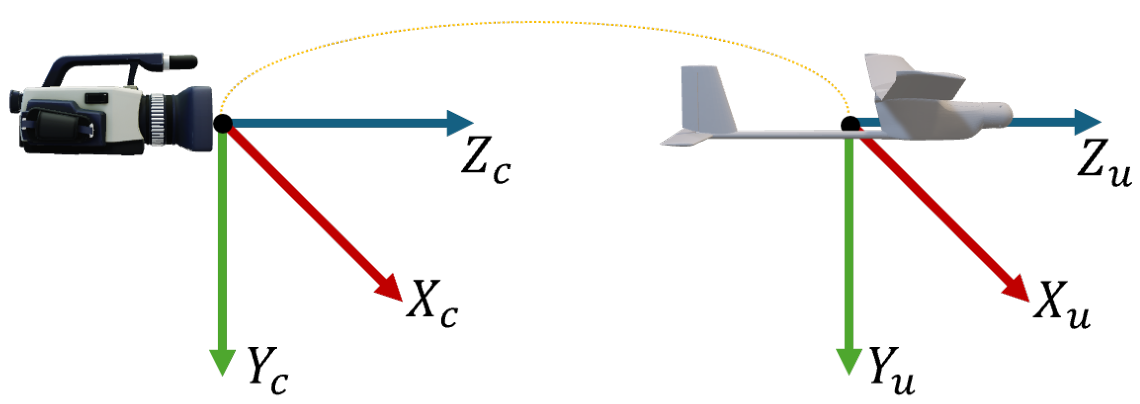The skew coefficient $\gamma$ is considered to be zero. The camera and UAV reference frames are depicted in Figure 5.

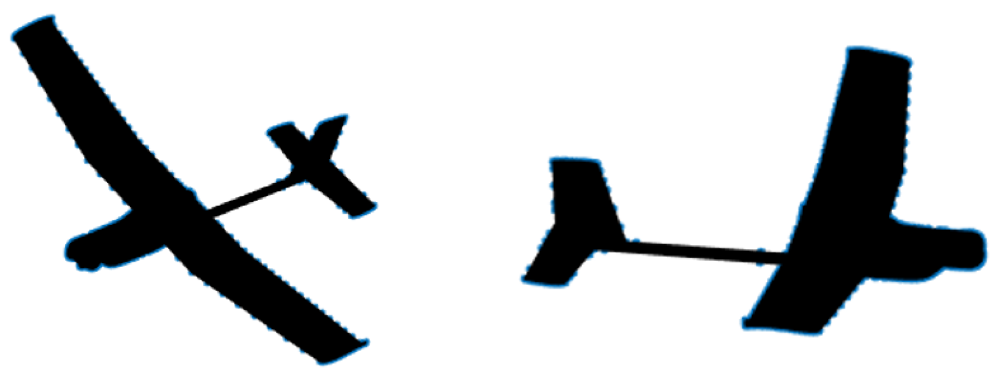
Both the chosen image size of 1280 width and 720 height ($1280\times 720$) and the intrinsic matrix parameters are consistent with those used in [26,27] for the purpose of performance comparison. By utilizing Equation (1), it becomes simple to create synthetic data for training algorithms and analyzing performance. Figure 6 illustrates two examples of binary images created using synthetic rendering. These binary images will be used as SOM input, as illustrated in Figure 3.

When capturing real-world images, considering the possibility of additional noise in the image when performing BS is important since a pre-processing step must ensure that it is minimized, not significantly influencing the SOM cluster detection. One way of performing this simple pre-processing is to use the Z-score [91,92]. Z-score is a statistical measure useful to quantify the distance between a data point and the mean of the provided dataset. The Z-score calculation can be obtained by [91,92]:

$${\mathbf{z}}_t={\displaystyle \frac{{\mathbf{x}}_t-{\mu }_t}{{\sigma }_t}}$$

(2)

where ${\mathbf{z}}_t$ represent the obtained Z-scores for a specific frame at time instant t, ${\mathbf{x}}_t={[{\mathit{\alpha }}_t^T,{\mathit{\beta }}_t^T]}^T$ describe the pixel coordinates that contain a binary value of 1 from the pre-processed binary image, ${\mu }_t$ denotes the mean of the pixel coordinates containing a binary value of 1, and ${\sigma }_t$ represents the Standard Deviation (SD) of the pixel coordinates containing a binary value of 1. Since we are dealing with $2D$ points in the image plane (frame) that represent pixels, we can compute the Euclidean distance from the origin to each point to be able to analyze each one using a single value. When the calculated distance for a certain point is below a predefined threshold $\lambda$, we can consider that point as part of our cluster. This technique, or another equivalent, has the primary objective of only selecting and using the pixels that belong to the UAV in the presence of noise, decreasing the obtained error, and obtaining a SOM input with lower error.

Each implementation case must be analyzed independently since, as expected, more errors usually result in a worse estimation. Therefore, it is essential to employ pre-processing with adequate complexity to deal with this kind of case. Most daily implementations have real-time processing requirements, and optimizing the system architecture to achieve them is essential.

3.2. Clustering Using a Self-Organizing Map (SOM)

A SOM allows the mapping of patterns known as input space onto a n-dimensional map of neurons known as output space [32,33,34,93]. In the intended application, the input space ${\mathbf{x}}_t={[{\mathit{\alpha }}_t^T,{\mathit{\beta }}_t^T]}^T$ at time instant t will be the pixel coordinates that contain a binary value of 1 from the pre-processed binary image. The binary image containing the UAV is represented by ${\mathbf{F}}_t^{BS}$, as illustrated in Figure 6, and has a size of $1280\times 720$. The output space will be a 2-dimensional map represented by a set of a predefined number of weights given by ${\mathbf{W}}_t$, that preserves the topological relations of the input space, as illustrated in Figure 3. The implemented SOM adapted to the problem at hand with all the proper descriptions of the definitions and notations is described in Algorithm 1.

Algorithm 1 Self-Organizing Map (SOM) [32,33,93]

1: Definitions & Notations: 2: Let $\mathbf{x}={[{\mathit{\alpha }}^T,{\mathit{\beta }}^T]}^T$ be the input vector, representing the 2D coordinates of the pixels that contain a binary value of 1 (input space). $\mathbf{x}$ consists of 2D pixels with coordinates u given by ${\mathit{\alpha }}^T$ and coordinates v given by ${\mathit{\beta }}^T$; 3: Let ${\mathbf{w}}_i={[{\mu }_i,{\nu }_i]}^T$ be the individual weight vector for neuron i; 4: Let $\mathbf{W}$ be the collection of all weight vectors ${\mathbf{w}}_i$ representing all the considered neurons (output space); 5: A SOM grid is a 2D grid where each neuron i has a fixed position and an associated weight vector ${\mathbf{w}}_i$. The grid assists in visualizing and organizing the neurons in a structured manner; 6: A Best Matching Unit (BMU) is the neuron b whose weight vector ${\mathbf{w}}_b$ is the closest to the input vector $\mathbf{x}$ regarding its Euclidean distance; 7: The initial learning rate is represented by ${\eta }_0$ and the final learning rate by ${\eta }_f$; 8: The total number of training epochs is given by $\Gamma$; 9: Let ${\mathbf{r}}_b$ and ${\mathbf{r}}_i$ be the position vectors of the BMU b and neuron i in the SOM grid, defined by their row and column coordinates in the grid; 10: Let $\sigma \left(e\right)$ be the neighborhood radius at epoch e, which decreases over time. 11: Input: $\mathbf{x}$ and the corresponding weight vectors $\mathbf{W}$. 12: Initialization: Initialize the weight vectors $\mathbf{W}$ randomly; Set the initial learning rate ${\eta }_0$, the final learning rate ${\eta }_f$, and the total number of epochs $\Gamma$. 13: Training - For each epoch $e=1$ to $\Gamma$: For each input vector $\mathbf{x}$: Competition: - Calculate the distance $d_i=\parallel \mathbf{x}-{\mathbf{w}}_i\parallel$ for all neurons i; - Identify the BMU ${\mathbf{w}}_b$ that minimizes the distance $b={argmin}_i\parallel \mathbf{x}-{\mathbf{w}}_i\parallel$; - Calculate the position vector ${\mathbf{r}}_b$ of the BMU b and the position vectors ${\mathbf{r}}_i$ of all neurons i in the SOM grid. Adaptation: - Update the weight vectors of the BMU and its neighbors to move closer to the input vector $\mathbf{x}$. The update rule is given by ${\mathbf{w}}_i^{(k+1)}={\mathbf{w}}_i^{\left(k\right)}+\eta \left(e\right)·h_{b,i}\left(e\right)·(\mathbf{x}-{\mathbf{w}}_i^{\left(k\right)})$; - Here, $\eta \left(e\right)$ is the learning rate at epoch e, which decreases over time, following $\eta \left(e\right)={\eta }_0{\left({\displaystyle \frac{{\eta }_f}{{\eta }_0}}\right)}^{{\displaystyle \frac{e}{\Gamma }}}$; - The neighborhood function $h_{b,i}\left(e\right)$ decreases with the distance between the BMU b and neuron i, modeled as Gaussian $h_{b,i}\left(e\right)=exp\left(-{\displaystyle \frac{\parallel {\mathbf{r}}_b-{\mathbf{r}}_i{\parallel }^2}{2{\sigma }^2\left(e\right)}}\right)$, where $\sigma \left(e\right)$ also decreases over time. 14: Output: The trained weight vectors $\mathbf{W}$ (output space) at the end of the training process represent the positions of the neurons in the input space after mapping the input data, as illustrated in Figure 7 and Figure 8.

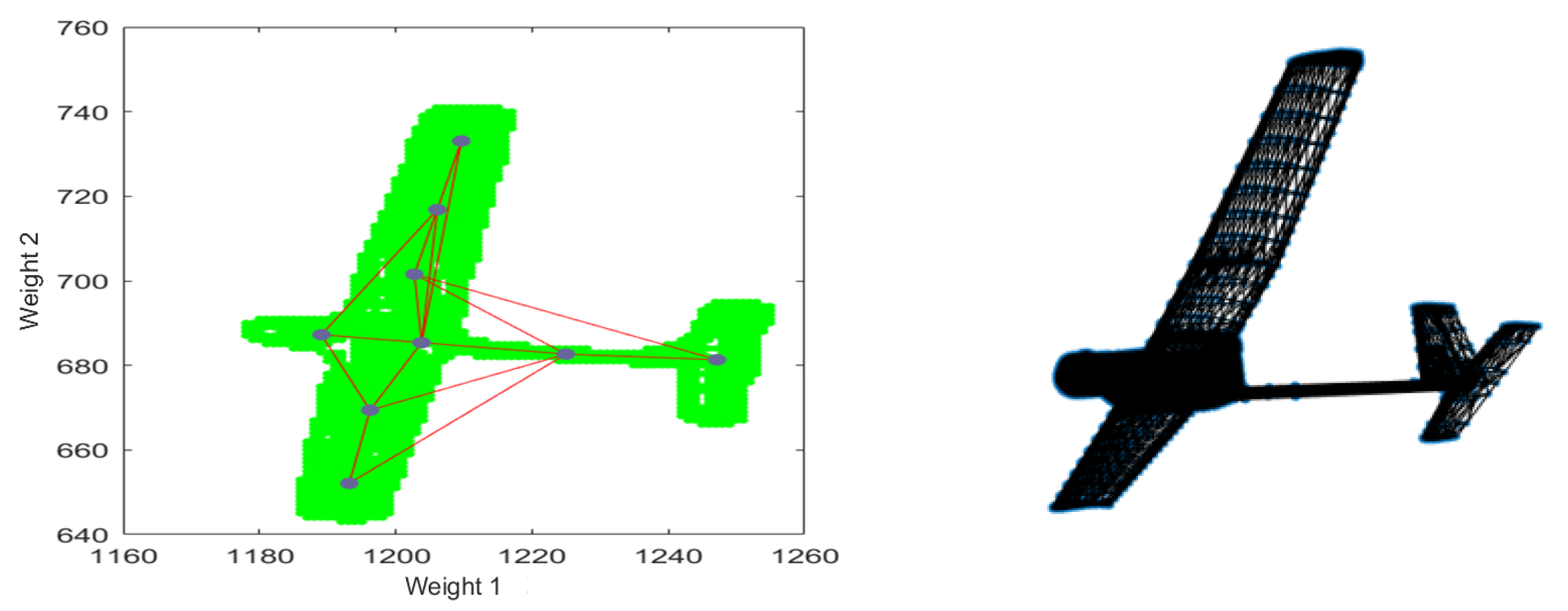
In Figure 7 and Figure 8, it is illustrated three different cases of the SOM output space after $\Gamma =250$ training epochs (iterations) with an initial learning rate of ${\eta }_0=0.1$ and a final learning rate of ${\eta }_f=0.05$ for two different examples. After analyzing the figures, it is possible to see a relationship between the output space given by the neuron positions represented by the dots and the topology of the input space in green. After analyzing Figure 7right, it is also possible to state that a higher number of neurons in the grid does not always represent our cluster or UAV better since, e.g., in the $4\times 4$ grid case, we have neurons located outside the considered input space that is represented using green color.

Figure 7. Example I of obtained clustering maps using SOM after 250 iterations: $2\times 2$ grid (left), $3\times 3$ grid (center) and $4\times 4$ grid (right). The dots represent the neuron positions according to their weights $\mathbf{W}$ (output space).

Figure 7. Example I of obtained clustering maps using SOM after 250 iterations: $2\times 2$ grid (left), $3\times 3$ grid (center) and $4\times 4$ grid (right). The dots represent the neuron positions according to their weights $\mathbf{W}$ (output space).

Figure 8. Example II of obtained clustering maps using SOM after 250 iterations: $2\times 2$ grid (left), $3\times 3$ grid (center) and $4\times 4$ grid (right). The dots represent the neuron positions according to their weights $\mathbf{W}$ (output space).

Figure 8. Example II of obtained clustering maps using SOM after 250 iterations: $2\times 2$ grid (left), $3\times 3$ grid (center) and $4\times 4$ grid (right). The dots represent the neuron positions according to their weights $\mathbf{W}$ (output space).

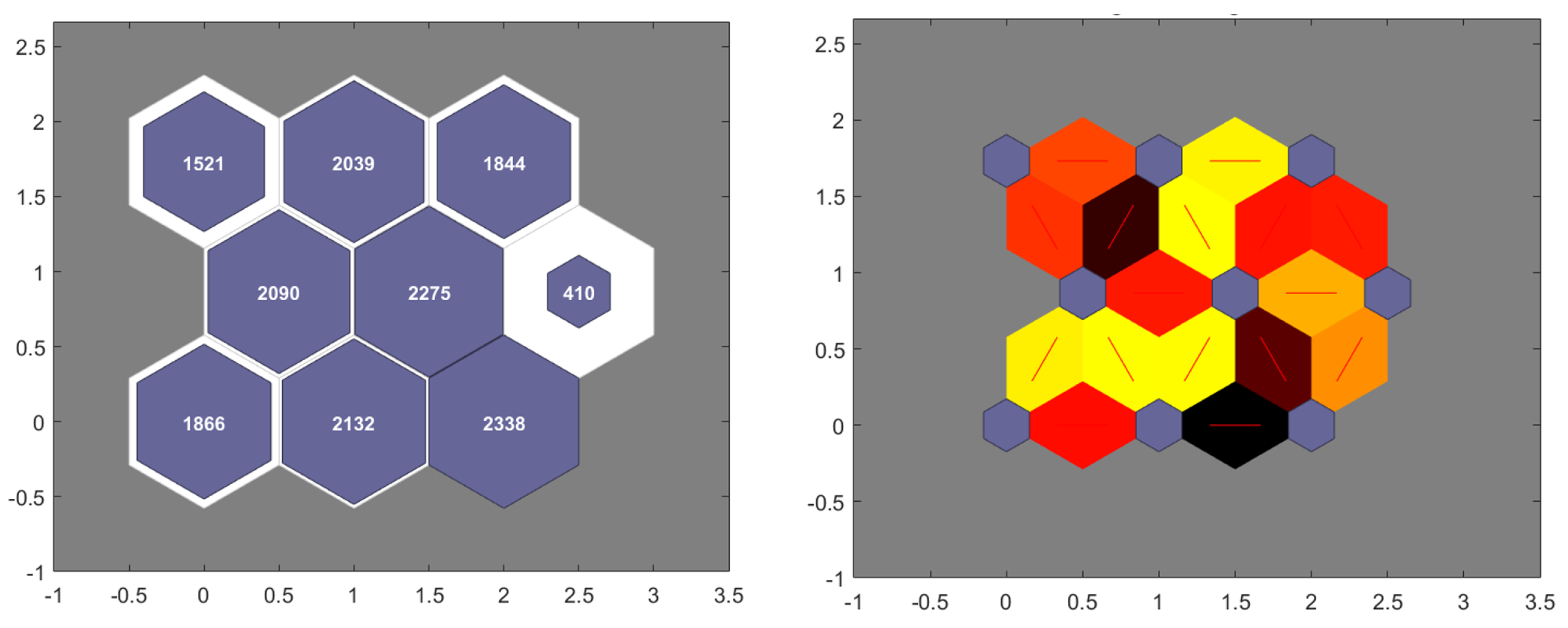
In Figure 9, it is illustrated the sample hit histogram and the neighbor distances map for the $3\times 3$ neuron grid (output space) shown in Figure 7 center. The sample hit histogram demonstrates the number of input vectors classified for each neuron, providing insight into the data distribution. The neighbor distances map illustrates the variance between adjacent neurons. The blue hexagons represent the neurons, the red lines depict the connections between neighboring neurons, and the colors indicate the distances, with darker colors representing larger distances and lighter colors representing smaller distances. Observing this data makes it possible to see that we have a cluster representation of the input space using a SOM, as needed and expected to be able to perform the pose estimation task.

It is possible to try to estimate the original UAV pose directly from the output space representing the input space topology, but it is not an easy task. It resembles trying to estimate an object’s pose considering a series of feature points with the advantage of being positioned according to the input space topology. Given the vast amount of possible UAV poses using, e.g., a pre-computed codebook [94] to try to estimate the UAV poses in a specific frame is impractical due to its dimension and can lead to a high error rate causing this estimate to have so much error that it cannot be used reliably.

3.3. Pose Estimation Using Deep Neural Networks (DNNs)

Using the SOM output space, it is possible to try to estimate the UAV pose using data obtained from a single frame. As briefly described before, and given the vast amount of possible UAV poses, using a pre-computed codebook of known poses is impractical [94]. DNNs are highly used nowadays in our daily lives and present a good capacity to solve complex and non-linear problems that generally will be unsolvable or need highly complex algorithm design. It is impractical to test all the possible network architectures, particularly since they are practically infinite without a parameter size limit. Since the output space of the SOM are weights that represent the topology of the input space, they can be considered as 2D feature points representing the input space.

To be able to use different loss functions, we have used almost the same network structure for translation and orientation but divided it into two different networks. Since we are dealing with weights that we have considered similar to 2D feature points, we have used Self-Attention (SA) layers [95,96], as described in Section 3.3.1, to consider the entire input and not a local neighborhood as usually considered in the standard convolutional layers. Also, when dealing with rotations and especially due to the quaternion representation, it was used a Quaternion Activation Function (QReLU) [97,98], as described in Section 3.3.3.

Section 3.3.1 will provide some notes about the common architecture layers used for translation and orientation estimation, Section 3.3.2 will describe the specific loss function and architecture used for the translation estimation, and finally, Section 3.3.3 will also describe the loss function and architecture used for the orientation estimation. Both used architectures are similar, with some adaptations to the task’s specificity.

3.3.1. General Description

SA layers were used in the adopted DNNs architectures to capture relations between the elements in the input sequence [95,96]. If we consider an input tensor $\mathbf{S}$ with shape $(H,W,C)$, where H is the height, W is the width, and C is the number of channels, the SA mechanism allows the model to attend to different parts of the input while considering their interdependencies (relationships). This approach is highly valuable when dealing with tasks that require capturing long-range dependencies or relationships between distant elements. The model can concentrate on relevant information and efficiently extract important features from the input data by calculating query and value tensors and implementing attention mechanisms. This enhances the model’s capacity to learn intricate patterns and relationships within the input sequence. The implemented SA layer is described in Algorithm 2.

Algorithm 2 Self-Attention Layer [95,96]

1: Definitions & Notations: 2: Let $\mathbf{S}$ be the input tensor with shape $(H,W,C)$, where H is the height, W is the width, and C is the number of channels; 3: Let f and h represent the convolution operations that produce the query and value tensors, respectively; 4: Let ${\mathbf{W}}_Q\in {\mathbb{R}}^{C\times {\displaystyle \frac{C}{8}}}$ and ${\mathbf{W}}_V\in {\mathbb{R}}^{C\times C}$ be the weight matrices for the query and value convolutions. 5: Input: $\mathbf{S}$ with shape $(H,W,C)$. 6: Initialization: Compute query and value tensors via $1\times 1$ convolutions: $$\begin{array}{cc}\hfill \mathbf{Q}& \leftarrow f\left(\mathbf{S}\right)=\mathbf{S}\ast {\mathbf{W}}_Q\hfill \\ \hfill \mathbf{V}& \leftarrow h\left(\mathbf{S}\right)=\mathbf{S}\ast {\mathbf{W}}_V\hfill \end{array}$$ 7: Attention scores calculation: Compute attention scores using a softmax function on the query tensor: $$\begin{array}{cc}\hfill {\mathbf{A}}_{i,j}& \leftarrow {\displaystyle \frac{exp\left({\mathbf{Q}}_{i,j}\right)}{{\sum }_{j^{\prime }}exp\left({\mathbf{Q}}_{i,j^{\prime }}\right)}}\hfill \end{array}$$ where i indexes the height and width dimensions, and j indexes the channels within the input tensor. The attention scores tensor $\mathbf{A}$ is reshaped and permuted to match the dimensions of $\mathbf{V}$. 8: Output: Compute the scaled value tensor via element-wise ⊙ multiplication: $$\begin{array}{cc}\hfill \mathbf{G}& \leftarrow \mathbf{V}\odot \mathbf{A}\hfill \end{array}$$ where $\mathbf{G}$ has shape $(H,W,C)$.

Both architectures for translation and orientation estimation share the same main architecture, only differing in the used loss functions and activation function since the orientation DNN use the QReLU activation function [97,98] near the output and performs quaternion normalization to ensure that the orientation estimation is valid, as will be explored in the next sections.

3.3.2. Translation Estimation

The translation estimation DNN is intended to estimate the vector ${\mathbf{T}}_t={[X,Y,Z]}^T$ at each instant t with low error. Given the SOM output, and taking into account the relations between the elements in the input sequence using SA layers, it was possible to create a DNN structure to perform this estimation, as illustrated in Figure 10. The details of each layer, its output shape, the number of parameters, and notes are described in Appendix A.

As illustrated in Figure 10, the proposed architecture primarily consists of 2D convolutions (Conv), SA layers (Attn), dropout to prevent overfitting (Dout), batch normalization to normalize the activations - neuron outputs (BN), and fully connected layers (FC). Since we want to estimate translations in meters, the implemented loss function was the Mean Square Error (MSE) between the labels (true value) and the obtained predictions. Although the structure seems complex, only the 2D convolution, the batch normalization, and the fully connected layers present trainable parameters, as described in

Table A1. DNN model used for the translation estimation summary.

Layer (Type)	Output Shape	Parameters	Notes	Label
Input	(3, 3, 2)	-	-	Input
2D Convolution	(3, 3, 64)	1216	-	Conv1
Batch Normalization	(3, 3, 64)	256	-	BN1
Activation (ReLU)	(3, 3, 64)	-	-	ReLU1
Self Attention	(3, 3, 64)	4689	-	Attn1
2D Convolution	(3, 3, 64)	36,928	-	Conv2
Batch Normalization	(3, 3, 64)	256	-	BN2
Activation (ReLU)	(3, 3, 64)	-	-	ReLU2
Self Attention	(3, 3, 64)	4689	-	Attn2
2D Convolution	(3, 3, 64)	36,928	-	Conv3
Batch Normalization	(3, 3, 64)	256	-	BN3
Activation (ReLU)	(3, 3, 64)	-	-	ReLU3
Self Attention	(3, 3, 64)	4689	-	Attn3
Dropout	(3, 3, 64)	-	0.5	Dout1
Self Attention	(3, 3, 64)	4689	-	Attn4
2D Convolution	(3, 3, 128)	73,856	-	Conv4
Batch Normalization	(3, 3, 128)	512	-	BN4
Activation (ReLU)	(3, 3, 128)	-	-	ReLU4
Self Attention	(3, 3, 128)	18,593	-	Attn5
2D Convolution	(3, 3, 128)	147,584	-	Conv5
Batch Normalization	(3, 3, 128)	512	-	BN5
Activation (ReLU)	(3, 3, 128)	-	-	ReLU5
Self Attention	(3, 3, 128)	18,593	-	Attn6
Dropout	(3, 3, 128)	-	0.5	Dout2
2D Convolution	(3, 3, 256)	295,168	-	Conv6
Batch Normalization	(3, 3, 256)	1024	-	BN6
Activation (ReLU)	(3, 3, 256)	-	-	ReLU6
2D Convolution	(3, 3, 256)	590,080	-	Conv7
Batch Normalization	(3, 3, 256)	1024	-	BN7
Activation (ReLU)	(3, 3, 256)	-	-	ReLU7
2D Convolution	(3, 3, 256)	590,080	-	Conv8
Batch Normalization	(3, 3, 256)	1024	-	BN8
Activation (ReLU)	(3, 3, 256)	-	-	ReLU8
Dropout	(3, 3, 256)	-	0.5	Dout3
Flatten	2304	-	-	Flatten
Fully Connected	512	1,180,160	ReLU, L2 ($\lambda =0.001$)	FC1
Dropout	512	-	0.5	Dout4
Fully Connected	256	131,328	ReLU, L2 ($\lambda =0.001$)	FC2
Dropout	256	-	0.5	Dout5
Fully Connected	3	771	Linear	Output

.

3.3.3. Orientation Estimation

The orientation estimation DNN is intended to estimate the vector ${\mathbf{O}}_t={[q_w,q_x,q_y,q_z]}^T$ at each instant t with low error. Given the SOM output, and taking into account the relations between the elements in the input sequence using SA layers, it was possible to create a DNN structure to perform estimation, as illustrated in Figure 11. The details of each layer, its output shape, the number of parameters, and notes are described in Appendix B.

As illustrated in Figure 11, the proposed architecture primarily consists of 2D convolutions (Conv), SA layers (Attn), dropout to prevent overfitting (Dout), batch normalization to normalize the activations—neuron outputs (BN), fully connected layers (FC), and a layer that obtains the quaternion normalization as the network output. Since we want to estimate orientation using a quaternion near the output, it was implemented the QReLU [97,98] activation function. The traditional Rectified Linear Unit (ReLU) activation function can lead to the dying ReLU problem, where neurons stop learning due to consistently negative inputs. QReLU addresses this issue by applying ReLU only to the real part of the quaternion, enhancing the robustness and performance of the neural network in the orientation estimation. Given a quaternion $\mathbf{q}={[q_w,q_x,q_y,q_z]}^T$, where $q_w$ represent the real part and ${[q_x,q_y,q_z]}^T$ the imaginary part, the QReLU can be defined as [97,98]:

$$\mathrm{QReLU}\left(\mathbf{q}\right)=\mathrm{QReLU}\left(\left[\begin{array}{c}{q}_w\\ q_x\\ q_y\\ q_z\end{array}\right]\right)=\left[\begin{array}{c}\mathrm{ReLU}\left(q_w\right)\\ q_x\\ q_y\\ q_z\end{array}\right]=\left[\begin{array}{c}max(0,q_w)\\ q_x\\ q_y\\ q_z\end{array}\right]$$

(3)

The adopted loss function $\mathcal{L}$ was the quaternion loss [99,100]. Given the true quaternion ${\mathbf{q}}_{\mathrm{true}}$ (label) and the predicted quaternion ${\mathbf{q}}_{\mathrm{pred}}$, it can be defined as [99,100]:

$$\mathcal{L}({\mathbf{q}}_{\mathrm{true}},{\mathbf{q}}_{\mathrm{pred}})={\displaystyle \frac{1}{N}}\sum _{i=1}^N\left(1-{\left({\displaystyle \frac{{\mathbf{q}}_{\mathrm{true},i}·{\mathbf{q}}_{\mathrm{pred},i}}{\parallel {\mathbf{q}}_{\mathrm{true},i}\parallel \parallel {\mathbf{q}}_{\mathrm{pred},i}\parallel }}\right)}^2\right)$$

(4)

where $\parallel \mathbf{q}\parallel =\sqrt{q_w^2+q_x^2+q_y^2+q_z^2}$ and the dot product ${\mathbf{q}}_{\mathrm{true},i}·{\mathbf{q}}_{\mathrm{pred},i}$ is given by:

$${\mathbf{q}}_{\mathrm{true},i}·{\mathbf{q}}_{\mathrm{pred},i}=q_{w,\mathrm{true},i}{q}_{w,\mathrm{pred},i}+q_{x,\mathrm{true},i}{q}_{x,\mathrm{pred},i}+q_{y,\mathrm{true},i}{q}_{y,\mathrm{pred},i}+q_{z,\mathrm{true},i}{q}_{z,\mathrm{pred},i}$$

(5)

By analyzing Equation (4), it is possible to state that it ensures the normalization of quaternions and computes the symmetric quaternion loss based on the dot product of normalized quaternions, averaged over all samples N. This is especially useful when we use batches during training. As described before, although the structure seems complex, only the 2D convolution, the batch normalization, and the fully connected layers present trainable parameters, as described in

Table A2. DNN model used for the orientation estimation summary.

Layer (Type)	Output Shape	Parameters	Notes	Label
Input	(3, 3, 2)	-	-	Input
2D Convolution	(3, 3, 64)	1216	-	Conv1
Batch Normalization	(3, 3, 64)	256	-	BN1
Activation (ReLU)	(3, 3, 64)	-	-	ReLU1
Self Attention	(3, 3, 64)	4689	-	Attn1
2D Convolution	(3, 3, 64)	36,928	-	Conv2
Batch Normalization	(3, 3, 64)	256	-	BN2
Activation (ReLU)	(3, 3, 64)	-	-	ReLU2
Self Attention	(3, 3, 64)	4689	-	Attn2
2D Convolution	(3, 3, 64)	36,928	-	Conv3
Batch Normalization	(3, 3, 64)	256	-	BN3
Activation (ReLU)	(3, 3, 64)	-	-	ReLU3
Self Attention	(3, 3, 64)	4689	-	Attn3
Dropout	(3, 3, 64)	-	0.5	Dout1
2D Convolution	(3, 3, 128)	73,856	-	Conv4
Batch Normalization	(3, 3, 128)	512	-	BN4
Activation (ReLU)	(3, 3, 128)	-	-	ReLU4
Self Attention	(3, 3, 128)	18,593	-	Attn4
2D Convolution	(3, 3, 128)	147,584	-	Conv5
Batch Normalization	(3, 3, 128)	512	-	BN5
Activation (ReLU)	(3, 3, 128)	-	-	ReLU5
Self Attention	(3, 3, 128)	18,593	-	Attn5
Dropout	(3, 3, 128)	-	0.5	Dout2
2D Convolution	(3, 3, 256)	295,168	-	Conv6
Batch Normalization	(3, 3, 256)	1024	-	BN6
Activation (ReLU)	(3, 3, 256)	-	-	ReLU6
2D Convolution	(3, 3, 256)	590,080	-	Conv7
Batch Normalization	(3, 3, 256)	1024	-	BN7
Activation (ReLU)	(3, 3, 256)	-	-	ReLU7
2D Convolution	(3, 3, 256)	590,080	-	Conv8
Batch Normalization	(3, 3, 256)	1024	-	BN8
Activation (ReLU)	(3, 3, 256)	-	-	ReLU8
Dropout	(3, 3, 256)	-	0.5	Dout3
Flatten	2304	-	-	Flatten
Fully Connected	512	1,180,160	-	FC1
Activation (QReLU)	512	-	-	QReLU1
Dropout	512	-	0.5	Dout4
Fully Connected	256	131,328	-	FC2
Activation (QReLU)	256	-	-	QReLU2
Dropout	256	-	0.5	Dout5
Fully Connected	4	1028	-	-
Normalization	4	-	Quaternion Normalization	Output

.

4. Experimental Results

This section presents experimental results to evaluate the performance of the developed architecture. Section 4.1 describes the used datasets, the network training process, and the parameters used. Section 4.2 explains the performance metrics adopted to quantify the results. Section 4.3 details the translation and orientation errors obtained, compares them with current state-of-the-art methods in RGB monocular UAV pose estimation using a single frame, and explores the system’s robustness in the presence of noise typical of real-world applications. Section 4.4 includes ablation studies to analyze the performance based on the adopted network structure. Section 4.5 provides some insights and analysis about applying the current system architecture to the real world. Finally, Section 4.6 presents a comprehensive overall analysis and discussion of the primary results achieved.

4.1. Datasets, Network Training & Parameters

Since there is no publicly available dataset with ground truth data and we have not been able to acquire an actual image dataset, we used a realistic synthetic dataset [101,102]. The system can then be applied to real data using transfer learning or by performing fine-tuning with the acquired real data. The training dataset contains 60,000 labeled inputs and was created using synthetically generated data, containing images with a size of $1280\times 720$. The synthetic data is created by rendering the UAV CAD model directly at the desired pose. This method ensures that the training dataset includes a wide range of scenarios and orientations. The ability to render the UAV in a wide range of poses and orientations using synthetic data enables the training of a robust and dependable model. The rendered poses vary in the following intervals: $X,Y\in [-1.5,1.5]$ m, and $Z\in [5,10]$ guaranteeing that the UAV is rendered on the generated frame. The synthetically generated pose orientations vary within the interval of $[-180,180]$ degrees around each Euler angle, as illustrated in Figure 5. In real captured frames, the obtained BS error could be decreased and ideally removed using the Z-score approach, as described in Section 3.1.

The considered SOM output space consisted of 9 neurons arranged in a $3\times 3$ grid, which were trained over 250 iterations, as detailed in Section 3.2. Our main goal was to estimate the UAV pose using 9 feature points ($3\times 3$ neuron grid) obtained from the SOMs output (output space). This number of feature points is reasonable considering the number of pixels available for clustering connected to the UAV distance to the camera.

During the training of the DNNs, the MSE was used as a loss function for translation estimation, and quaternion loss was utilized as a loss function for orientation estimation, as described in Section 3.3. 80% of the dataset was used for training and 20% for validation over 50,000 iterations using the Adaptive Moment Estimation (ADAM) optimizer and a batch size of 256 images. As expected, the loss decreased during training, with a significant reduction observed during the initial iterations, as described in Section 4.4. Minor adjustments were performed during the remainder of the training to optimize the trainable parameter values and minimize errors. The pose estimation performance analysis used three different datasets of 850 poses at $Z=5,7.5,$ and 10, with X and Y varying within the intervals of $[-0.5,0.5]$ m and Euler angles within the interval of $[-180,180]$ degrees.

4.2. Performance Metrics

The algorithms were implemented on a 3.70 GHz Intel i7-8700K Central Processing Unit (CPU) and NVIDIA Quadro P5000 with a bandwidth of 288.5 GB/s and a pixel rate of 110.9 GPixel/s. The obtained processing time was not a performance metric since we used a ground-based system without power limitations and easy access to high processing capabilities. Although this is not a design restriction, a simple system was developed to allow the system implementation without requiring high computational resources.

The translation error between the estimated poses and the ground truth labels was determined using the Euclidean distance. In contrast, the quaternion error ${\mathbf{q}}_{\mathrm{error}}$ was calculated as follows:

$${\mathbf{q}}_{\mathrm{error}}={\mathbf{q}}_{\mathrm{true}}\otimes {\overline{\mathbf{q}}}_{\mathrm{pred}}$$

(6)

where ⊗ represents the unit quaternion multiplication, ${\mathbf{q}}_{\mathrm{true}}$ represents the ground truth, and ${\overline{\mathbf{q}}}_{\mathrm{pred}}$ represents the conjugate of the predicted quaternion (estimate). The angular distance in radians corresponding to the orientation error is obtained by:

$${\theta }_{\mathrm{radians}}=2·arccos\left(\right|{\mathbf{q}}_{\mathrm{error}}\left|\right)$$

(7)

where ${\theta }_{\mathrm{radians}}$ is them converted into degrees ${\theta }_{\mathrm{degrees}}$ to be analyzed. Both translation and orientation errors were analyzed using Median, Mean Absolute Error (MAE), SD, and Root Mean Square Error (RMSE) [103].

4.3. Pose Estimation Error

Given three different datasets of 850 poses, as described in Section 4.1, the pose estimation error was analyzed at different camera distances using the performance metrics described in Section 4.2. Estimating the UAV pose with low error is essential to automate important operational tasks such as autonomous landing.

When analyzing

Table 1. Obtained translation error in meters.

Distance	Minimum	Median	Maximum	MAE	RMSE	SD
5	0.10	0.28	1.25	0.32	0.34	0.14
7.5	0.02	0.25	1.93	0.33	0.42	0.26
10	0.14	0.42	2.34	0.49	0.56	0.27

, it is clear that the translation error increases as the distance from the camera increases. The greatest error occurs in the Z coordinate since the scale factor is difficult to estimate. However, the performance is still satisfactory, with a low error of around 0.33 m as indicated by the obtained MAE at distances of 5 and 7.5 m.

By analyzing

Table 2. Obtained orientation error in degrees.

Distance	Minimum	Median	Maximum	MAE	RMSE	SD
5	0.77	14.77	179.8	29.26	47.44	37.37
7.5	1.81	14.31	178.7	28.34	45.98	36.23
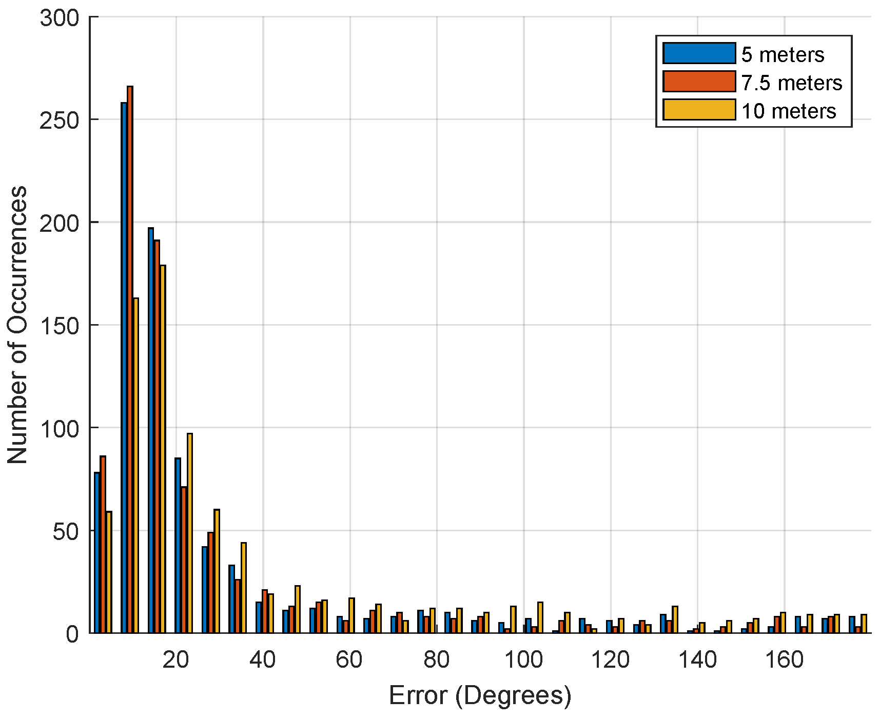
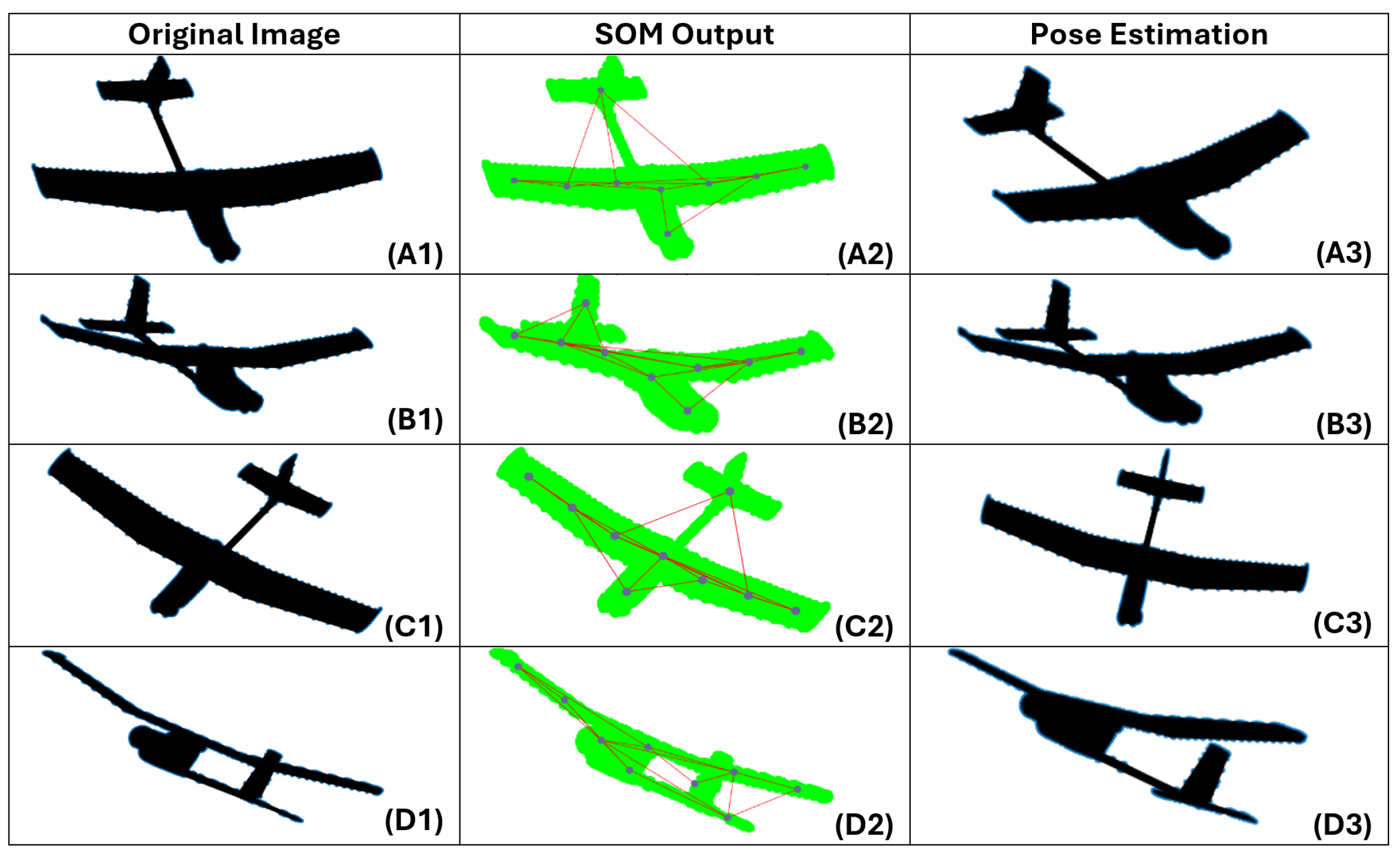
10	0.98	19.88	178.1	39.71	59.01	43.68

, it is evident that the orientation error also increases with the camera distance but at a lower rate than the observed for the translation. A MAE of approximately 29 degrees at distances of 5 and 7.5 m was obtained. The maximum error is observed near 180 degrees, primarily due to the UAV’s symmetry. It makes it difficult to differentiate between symmetric poses because the rendered pixels present almost the same topology, as illustrated in Figure 12.

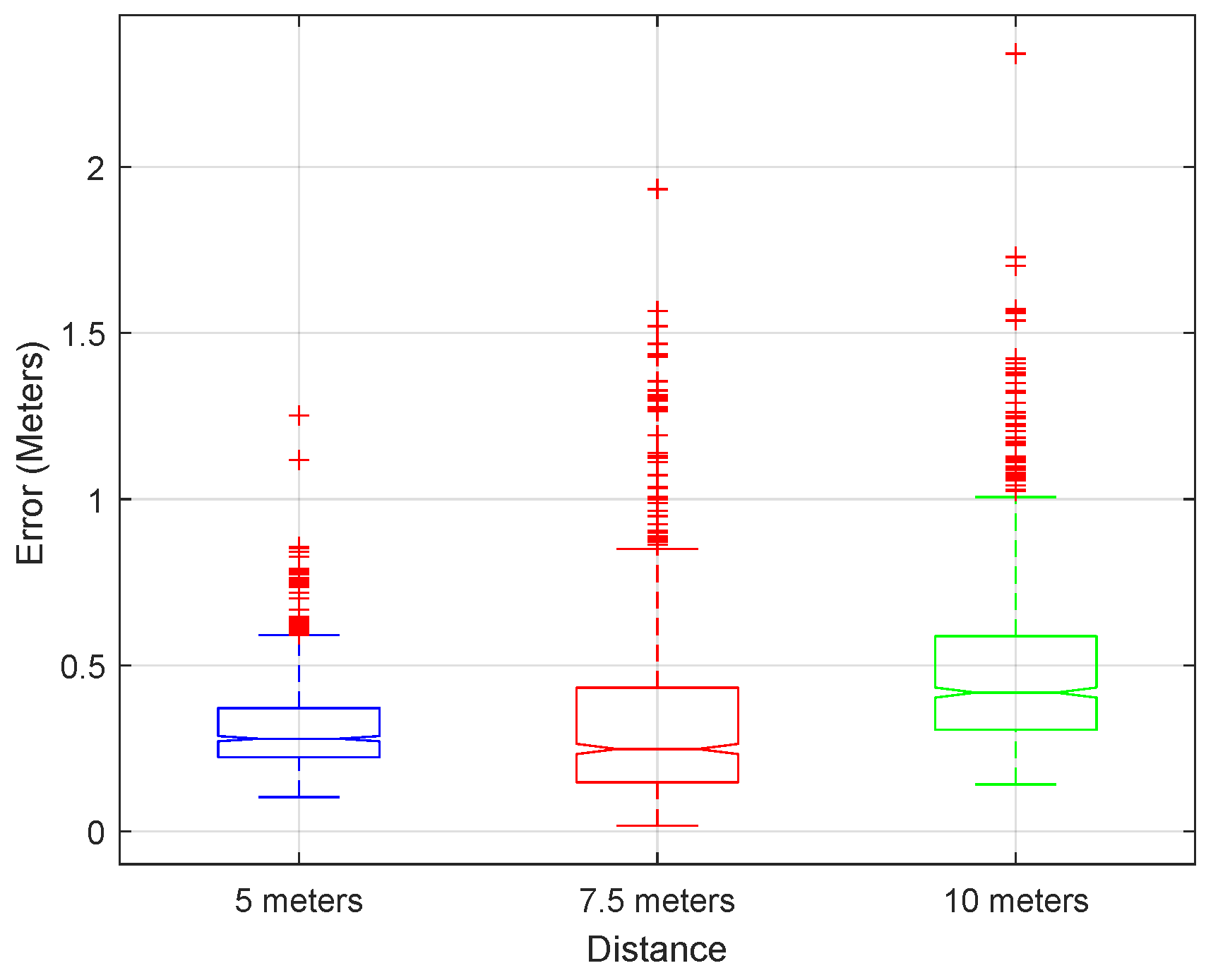
The translation error boxplot is illustrated in Figure 13, where we can see the existence of some outliers. Still, most of the translation estimations are near the median, as described before. On the other hand, when analyzing the orientation error histogram, as illustrated in Figure 14, we can see that the vast majority of the error is near zero degrees, as expected.

Some examples of pose estimation using the proposed architecture are illustrated in Figure 15, demonstrating the good orientation performance obtained by the proposed method. As described earlier and illustrated in Figure 14, some bad estimations and outliers will exist, but they can be reduced using temporal filtering [23].

4.3.1. Comparison with Other Methods

It is possible to compare the proposed system with other state-of-the-art RGB ground-based UAV pose estimation systems. In [26], a PF based approach using 100 particles is employed, enhanced by optimization steps using a Genetic Algorithm based Framework (GAbF). In [27], three pose optimization techniques are explored under different conditions from those in [26], namely Particle Filter Optimization (PFO), a modified Particle Swarm Optimization (PSO) version, and the GAbF again. These applications do not perform pose estimation in a single shot, relying on pose optimization steps using the obtained frame.

When we compare the translation error achieved by the current state-of-the-art ground-based UAV UAV pose estimation systems using RGB data, as outlined in

Table 3. Translation error comparison in meters with current state-of-the-art applications at 5 m.

Method	Median	MAE
SOM + DNN (Ours)	0.28	0.32
GAbF [26]	0.27	0.19
PFO [27]	0.00	0.21
Modified PSO [27]	0.00	0.18
GAbF [27]	0.01	0.09

, it becomes apparent that the used optimization algorithms in [26,27] result in more accurate translation estimates. This is primarily attributed to optimizing the estimate using multiple filter iterations on the same frame, which allows for a better scale factor adjustment and consequently provides a more accurate translation estimation. However, it should be noted that we are discussing very small errors that are suitable for most trajectory guidance applications [23].

The main advantage is verified in orientation estimation, as shown in

Table 4. Orientation error comparison in degrees with current state-of-the-art applications at 5 m.

Method	Median	MAE
SOM + DNN (Ours)	14.77	29.26
GAbF [26]	14.6	37.2
PFO [27]	1.47	94.26
Modified PSO [27]	0.30	97.37
GAbF [27]	2.71	89.22

, where the obtained MAE is, on average, 2.72 times smaller than that achieved by the state-of-the-art methods. It is important to note that these results are obtained in a single shot without any post-processing or optimization, unlike the considered algorithms that rely on a local optimization stage. The obtained results can be further improved using temporal filtering, as multiple frame information can enhance the current pose estimation [19].

As far as we know, no other publicly available implementations of single-frame RGB monocular pose estimation exist for a proper comparative analysis. Therefore, we chose these methods for comparison.

4.3.2. Noise Robustness

In real-world applications, it is typical to have noise present that can affect the estimate. As described before, the main focus of this article is not on the BS algorithm and methods but rather on using this data to perform single-frame monocular RGB pose estimation by combining a SOM with DNNs. To analyze the performance of the DNN in the presence of noise, a Gaussian distribution with mean zero ($\mu =0$) and different values of SD ($\sigma$) was added to the obtained weights (SOM output), and the resulting error was analyzed. Adding noise to the output space of the SOM is equivalent to adding noise to the original image since the final product of this noise will be a direct error in the cluster topology represented by the weights. Given the three different datasets of 850 poses, as described in Section 4.1, the pose estimation error was analyzed at different camera distances and with the addition of Gaussian noise using the performance metrics described in Section 4.2.

By analyzing

Table 5. Translation error at 5 m when varying the Gaussian noise SD (meters).

Noise SD	Minimum	Median	Maximum	MAE	RMSE	SD
1	0.10	0.28	1.29	0.32	0.34	0.14
5	0.09	0.28	1.17	0.32	0.35	0.15
10	0.09	0.28	1.66	0.33	0.37	0.16
15	0.11	0.28	1.69	0.34	0.39	0.19
30	0.09	0.29	2.04	0.37	0.45	0.25
50	0.09	0.32	3.37	0.41	0.50	0.28
100	0.13	0.52	3.82	0.66	0.82	0.49
200	0.17	0.91	4.04	1.10	1.25	0.60

, it is clear that there is a direct relationship between the obtained error and the added Gaussian noise SD, as the error increases with the increase in the SD value. The RMSE increases by approximately 47.1%, the MAE increases by approximately 28.1%, and the maximum obtained error increases by approximately 161.2% when varying the noise SD from one to 50. Additionally, the network demonstrates remarkable robustness to noise, as adding Gaussian noise with a $\sigma =50$ significantly changes the weights’ positions. However, the DNN can still interpret and retrieve scale information from them.

After analyzing

Table 6. Orientation error at 5 m when varying the Gaussian noise SD (degrees).

Noise SD	Minimum	Median	Maximum	MAE	RMSE	SD
1	1.54	14.68	179.20	29.29	47.44	37.34
5	1.86	15.67	179.40	32.60	51.93	40.45
10	1.52	21.85	179.86	41.72	61.00	44.53
15	2.19	30.93	179.79	54.37	73.83	49.97
30	2.86	86.07	179.89	90.74	106.04	54.92
50	7.76	120.26	179.70	110.77	121.11	48.99
100	12.56	132.39	179.82	125.64	131.95	40.36
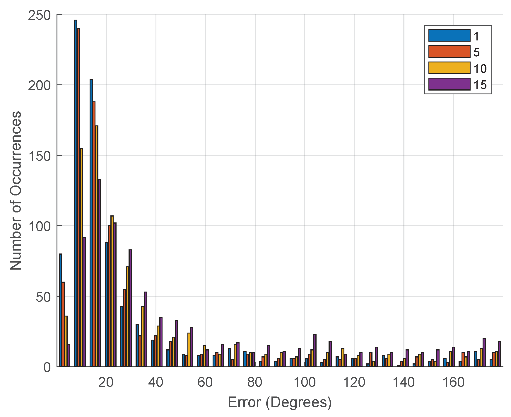
200	6.77	134.47	180.00	126.00	132.12	39.80

, it is evident that the orientation estimation is highly affected by the weights’ topology (SOM output space), as expected. The RMSE increases by approximately 55.6%, and the MAE increases by approximately 85.6% when varying the noise SD from one to 15. The topology is randomly changed when Gaussian noise is added to the weights, and the orientation estimation error increases. However, the error remains acceptable even without temporal filtering [23] and relying solely on single-frame information since the considered sigmas provide a significant random change in the weight values. Figure 16 illustrates the orientation error histogram obtained when changing the SD. It is evident that as the SD increases, the orientation error also increases, resulting in more non-zero error values.

4.4. Ablation Studies: Network Structure

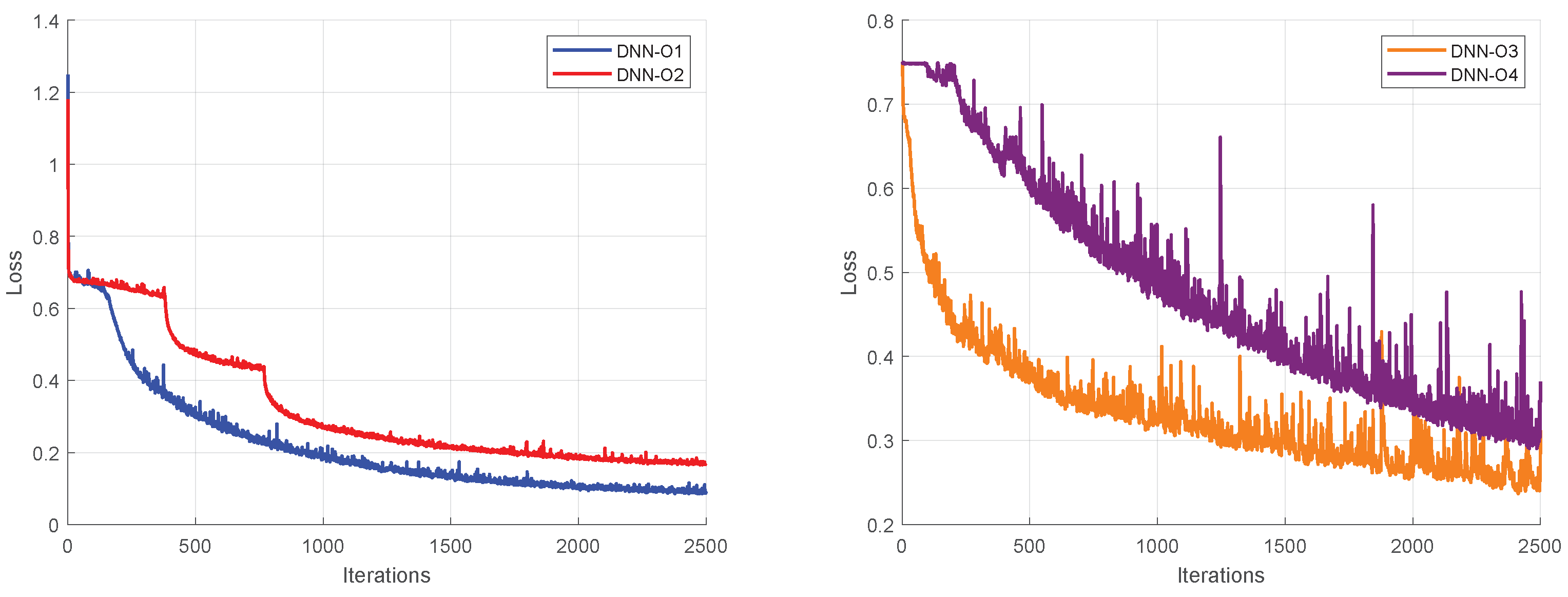
In this section, we conducted ablation studies to evaluate the impact of each layer in the network structure on the training process. We analyzed how each layer influenced the network learning during training. We systematically removed layers from the proposed architecture during the ablation studies to understand their contribution during training. The network was trained for 2500 iterations using the dataset containing 60,000 labeled inputs described in Section 4.1.

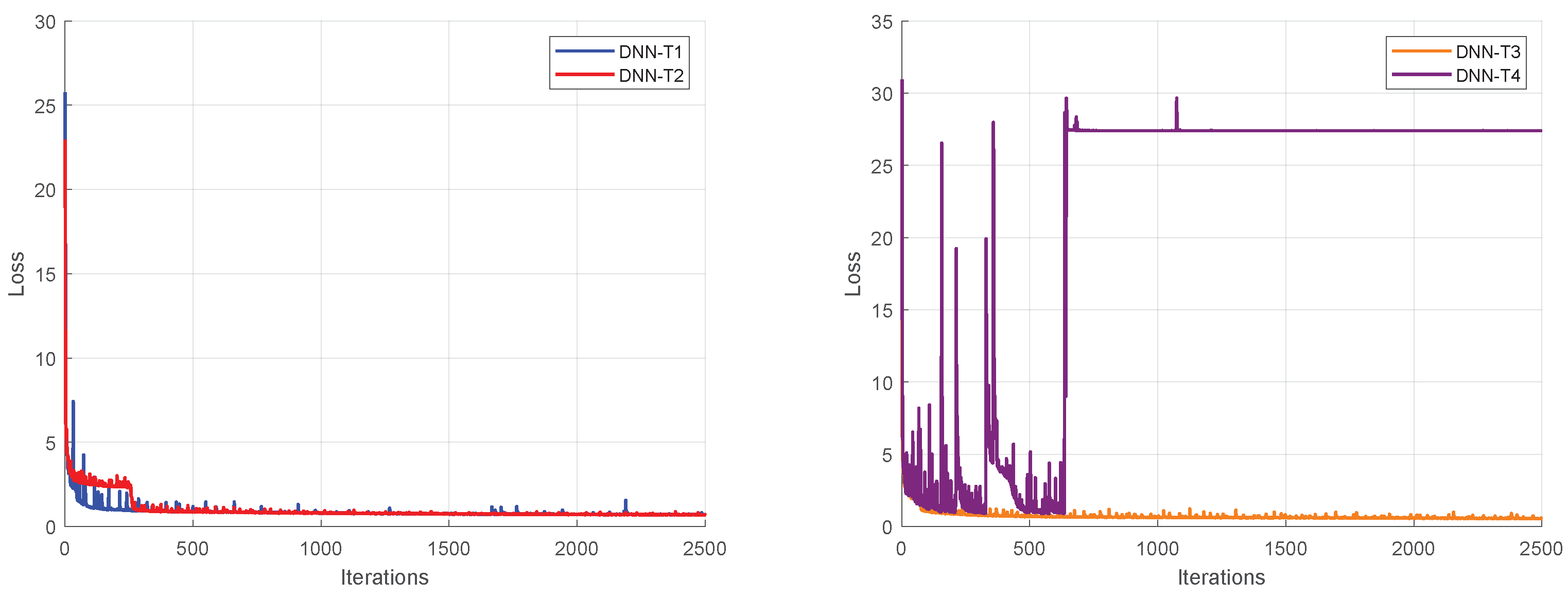
For the translation DNN analysis, the network layers were removed according to the described in

Table 7. Summary of DNN models for translation estimation used for ablation studies.

Name	Variant
DNN-T1	Considered DNN for translation estimation without any change
DNN-T2	Removing the SA layers
DNN-T3	Removing the SA layers & the kernel regularizers
DNN-T4	Removing the SA layers & the kernel regularizers & the batch normalization layers

. From the analysis of Figure 17, it is possible to state that the training loss obtained by the MSE is slightly affected when using DNN-T2 and DNN-T3. Still, when removing the batch normalization layers DNN-T4, the network cannot learn from its inputs, justifying its use in the proposed structure.

The network layers were removed according to the description in

Table 8. Summary of DNN models for orientation estimation used for ablation studies.

Name	Variant
DNN-O1	Considered DNN for orientation estimation without any change
DNN-O2	Removing the SA layers
DNN-O3	Removing the SA layers & the kernel regularizers
DNN-O4	Removing the SA layers & the kernel regularizers & the batch normalization layers

for the orientation DNN analysis. Analysis of Figure 18 indicates that training is significantly affected by removing network components. The importance of the SA block is evident, as it allows for better capture of the relationship between input elements, which is particularly important for orientation estimation. Since the loss is determined by the quaternion loss, seemingly minor differences in the obtained values represent major differences obtained during training and, consequently, during the estimation process.

4.5. Qualitative Analysis of Real Data

Due to the absence of ground-truth real data, only a simple qualitative analysis was possible. Figure 19 shows the original captured frame and the result of implementing a BS algorithm. It is easily perceptible that the UAV in the captured frame is located at a higher distance than those used in the synthetic dataset generated for training our DNN.

A qualitative comparison of the obtained result with the original frame is also possible. From the analysis of Figure 20, some pose error is evident. Still, the orientation error is acceptable and can be minimized by training the DNNs with more samples at higher distances and performing fine-tuning with a real captured dataset. It is important to note that we are not implementing any algorithm to fine-tune the obtained pose estimation. Instead, we consider the SOM output space as 9 feature points and use only that information to perform pose estimation. Due to the considered UAV distance to the camera, the number of used feature points was considered fixed at 9 ($3\times 3$ grid). For higher distances, the need to use fewer points should be analyzed as the pixel image information becomes too low, and more points do not bring any additional information.

It is important to state that the system can be trained using synthetic data to obtain better performances in real-world scenarios and then fine-tuned using real data to ensure high pose estimation accuracy.

4.6. Overall Analysis & Discussion

We have implemented an architecture that performs single-frame RGB monocular pose estimation without relying on additional data or information. The proposed system demonstrates comparable performance and superior orientation estimation accuracy compared with other state-of-the-art methods [26,27]. As described in Section 4.3.2, and as expected, the addition of noise increases the pose estimation error since the pose estimation is dependent on the SOM output space topology. However, the system demonstrates overall good performance and acceptable robustness to noise. As described in Section 3, testing all possible network structures and implementations is impractical due to the almost infinite possibilities. The system was developed as a small network with limited trainable parameters, allowing it to be implemented on devices with low processing power capabilities if needed while maintaining high accuracy. For example, in fixed-wing autonomous landing operations in net-based retention systems [16,23], the typical landing area is about $5\times 6$ m, and the developed system’s accuracy is sufficient to meet this requirement. Including a temporal filtering architecture [8,18] that relies on information from multiple frames using temporal filtering can improve results, as the physical change in UAV pose between successive frames is limited.

5. Conclusions

A new architecture for single RGB frame UAV pose estimation has been developed based on a hybrid ANN model, enabling essential estimates to automate mission tasks such as autonomous landing. High accuracy is achieved by combining a SOM with DNNs, and the results can be further improved by incorporating temporal filtering in the estimation process. This work fixed the SOM grid at $3\times 3$, representing its output space and DNNs input. Future research could adapt the grid size to the UAV’s distance from the camera and combine multiple SOM output grids for better pose estimation, investigating the impact of different grid sizes and configurations to optimize computational efficiency and accuracy. Additionally, incorporating temporal filtering to utilize information between frames can smooth out estimation noise and enhance robustness. Integrating additional sensor data, such as Light Detection And Ranging (LIDAR), Infrared Radiation (IR) cameras, or Inertial Measurement Units (IMUs), could provide a more comprehensive understanding of the UAV’s environment and further enhance accuracy. However, this was not explored here since one of the objectives was to maintain robustness against jamming actions using only CV. The architecture’s application can extend beyond autonomous landing to tasks such as obstacle avoidance, navigation in GPS-denied environments, and precise maneuvering in complex terrains. Continuous development and testing in diverse real-world scenarios is essential to validate the system’s robustness and versatility. In conclusion, the proposed hybrid ANN model for single RGB frame UAV pose estimation represents a significant advancement in the field, with the potential to greatly improve the reliability of UAV operations.