Technical Note

Image-to-Image Translation-Based Deep Learning Application for Object Identification in Industrial Robot Systems

1
Department of Vehicles Engineering, Faculty of Engineering, University of Debrecen, Ótemető Str. 2–4, 4028 Debrecen, Hungary
2
Department of Data Science and Visualization, Faculty of Informatics, University of Debrecen, Kassai Str. 26, 4028 Debrecen, Hungary
*
Author to whom correspondence should be addressed.
Robotics 2024, 13(6), 88; https://doi.org/10.3390/robotics13060088
Submission received: 29 March 2024 / Revised: 24 May 2024 / Accepted: 27 May 2024 / Published: 2 June 2024
(This article belongs to the Topic Smart Production in Terms of Industry 4.0 and 5.0)

Abstract

:
Industry 4.0 has become one of the most dominant research areas in industrial science today. Many industrial machinery units do not have modern standards that allow for the use of image analysis techniques in their commissioning. Intelligent material handling, sorting, and object recognition are not possible with the machinery we have. We therefore propose a novel deep learning approach for existing robotic devices that can be applied to future robots without modification. In the implementation, 3D CAD models of the PCB relay modules to be recognized are also designed for the implantation machine. Alternatively, we developed and manufactured parts for the assembly of aluminum profiles using FDM 3D printing technology, specifically for sorting purposes. We also apply deep learning algorithms based on the 3D CAD models to generate a dataset of objects for categorization using CGI rendering. We generate two datasets and apply image-to-image translation techniques to train deep learning algorithms. The synthesis achieved sufficient information content and quality in the synthesized images to train deep learning algorithms efficiently with them. As a result, we propose a dataset translation method that is suitable for situations in which regenerating the original dataset can be challenging. The results obtained are analyzed and evaluated for the dataset.

1. Introduction

In industry, there are a lot of old machine units in use whose applicability could be extended. Robots on production lines are mechanically capable of performing various machining and logistic tasks. Their limitations are mainly on the software side, as one of the foundations of Industry 4.0 is network-based communication and monitoring, which is difficult to implement [1]. Furthermore, the higher computational demands of deep learning-based imaging tasks cannot be met by traditional solutions. Several studies have shown examples of the use of deep learning for legacy robotic units.
Deep learning has enhanced the basic functionality of an older ABB IRB2400L in one of the studies, allowing for more efficient data processing [2]. In a similar industrial context, neural networks have been applied to a two-armed robot unit called Baxter. One of the primary reasons for this was that it was an older model, and the factory sensor units provided limited options for object detection. Therefore, the F-SIOL-310 dataset was created to improve the object detection rate [3]. The use of neural networks is also a key focus in the development of warehousing systems. In one case, an old Toshiba Machine VL500 7 DOF performed sorting tasks so that the boxes were texture-less [4]. In some cases, such as the Franka Emika Panda medical robot [5], a simulation framework first learns a model before implementing it in a real environment.
Generally, vision sensors and neural networks have been used to make these robots smart [6].
In the case of multi-axis robotic arms, the same detection of object displacement is required as in the case of mobile vehicles to perform evasive maneuvers [7]. However, an important difference is that in the workspace of robotic units, the conveyor belts that transport the raw materials are on constrained paths. In this paper, an assembly line robot unit performing material handling tasks in two application areas is used to develop a method to enable legacy machine units to perform deep learning-based image analysis tasks. One of the multi-axis robots is the KUKA KR5 [8] with a Flexlink XK conveyor in its workspace, while the other is the Sony SCARA SRX-611 [9] with a PARO QE 01 31-6000 conveyor belt (see also Figure 1).
During the implementation, sample test pieces will be designed and manufactured on-site using a 3D printer and additive manufacturing technology. The parts that pass on the conveyor belts will be detected using our own trained neural network.
While machine learning techniques can provide robust and reliable solutions to problems that are difficult or less well-addressed by classical algorithms, the right dataset is always a crucial part of the training process. In the prior related work [10], the possibilities of extending the functionality of older robots were also discussed based on a deep learning-based neural network, and a learning dataset was generated based on rendering methods and achieved reasonable accuracy; however, when examined on real images, the accuracy of the trained algorithms was significantly degraded in cases in which the real images were really different and in which other phenomena, such as reflections, various distortions, illumination, and color variations, etc., occurred in large quantities. The reason is that the quality of the image data and the information content of the dataset itself significantly determine the accuracy of the training and whether we can provide the most general procedure possible. In our case, the image dataset used for training deep learning algorithms is produced using data synthesis, more specifically using data synthesis based on image-to-image translation techniques, to achieve the most realistic results possible. Thus, based on the information content and quality of the synthesized images, we can measure the threshold that must be reached during the synthesis in order to train deep learning algorithms with sufficient accuracy. Moreover, based on our work, we propose a dataset translation procedure, which will mostly be applicable in cases in which the regeneration of datasets can become difficult or impossible in the future. In order to run the trained neural network, the necessary computational hardware specifications must be determined, too.
The rest of this work is structured as follows: The technical background of the multi-axis robot units and conveyor belts is described in Section 2. Section 3 describes the dataset translation method, including the theoretical background and the model. Section 4 presents the in-house-developed FDM 3D printer and test object printing. It also discusses creating a dataset to train a neural network with real and rendered images. The architecture description of the chosen detectors is enclosed in Section 5. Section 6 describes the settings and parameter adjustments made during training and summarizes the results of deep learning-based algorithms, depending on the results. Conclusions are drawn in Section 7.

2. Multi-Axis Robot Units and Conveyor Belts

First of all, we have to discuss the old devices and their configuration because our developed methodology depends on the primary hardware environment, and we have to optimize it to improve devices into smart devices (for details, see Figures 7 and 13).
The industrial assembly line available in our robotics laboratory, which is a member of the Flexlink XK pallet system, was used in the project. It is typically used in the automotive industry to perform logistics tasks [11]. The main advantages of the industrial plastic conveyor manufactured by Flexlink XK are the short delivery time and the flexible modular design. The low weight of the aluminum cube placed by the robot does not cause any difficulties for the conveyor belt, as it has a load capacity of up to nearly 10 kg. The plastic belt part itself is 45 mm wide and nearly 5200 mm long [12].
Also, part of the robot cell system is the KUKA KR5 robot unit in the middle, which is also widely used in the automotive industry. The robot design is mainly used for arc welding tasks.
It has a working envelope volume of 8.4 m3, which makes it suitable for complex tasks, and has a repeatability of 0.04 mm. The robot has six axes and weighs 127 kg. The payload of the gripper element is 5 kg. With the help of the KUKA KR5 Gmbh electro-pneumatic gripper itself, it is able to load the parts onto the Flexlink XK conveyor in its work area, which then performs the transport task. Around the robot arm, a robot cell was built from aluminum profiles, which included a Flexlink XK conveyor belt.
The other robot unit is the Sony SCARA SRX-611, which is used for logistics tasks in the industry. The robot arm has a weight of 35 kg and a payload of 2 kg, which will be considered when designing 3D-printed sample workpieces. In this case, the gripper is also electro-pneumatic, and a PARO QE 01 31-6000 [13] conveyor belt installed in the workroom ensures the transport of the pallets, which is equipped with four additional stop mechanisms, each with an inductive sensor.

3. Dataset Translation Method

This section explains more about the dataset translation technique to create realistic images.
Firstly, we provide an overview of the most relevant publications and theoretical backgrounds for image descriptiveness. After that, we introduce a theoretical model that describes in detail the main components of a realistic image.
As a result, we present our proposed image-to-image translation-based deep learning method, which we have transformed and optimized according to the given application.

3.1. Related Works

In all cases in which real image recordings are examined, a number of specific phenomena, such as reflections, color variations, and various light phenomena, can be observed in the images, which are caused by specific environmental effects, either by the specific characteristics of the object and its environment or by the specific lens system architecture of the image capture device. In the latter case, in which the physical properties and parameters are not disclosed by the device maker, it is extremely difficult to build a theoretical model for each unique system [14,15]. From an illumination standpoint, optimum circumstances can be set in many manufacturing processes [16], but as Martinez et al. pointed out in their work on an automated steel production process supported by visual sensors, there can be restrictions on the components to be produced [17]. Given the above reasons, it is necessary to first characterize the phenomena discovered in the real image in order to explore and suggest a robust solution to the resulting problems. Formally, the following relationship [18] describes a real image (see Figure 2):
I r e a l = I n o r m a l + I p h e n o n e m a + N 0 ,   σ 2 ,
where I n o r m a l denotes the feature-free image inversion component, I p h e n o m e n a denotes the feature-containing image component separately, and N denotes a random Gaussian noise, whose variance is sampled from a scaled chi-square distribution as σ 2 0.01 χ 2 .
Reflections and flares are the two basic categories for the components that contain individual phenomena. Extreme lighting conditions cause reflections to form on the surface of the camera system’s lenses. Their form and frequency are mostly determined by the lens system’s design. They can be classified into two groups based on their type as follows: scattered and reflective. This phenomenon is far less likely to occur in production processes, in which illumination is highly regulated, and it can impede object detection. Nonetheless, it is essential to keep in mind that when it occurs, it might result in severely burned-out pixel areas, which can considerably influence the performance of machine learning algorithms and aggravate the loss of detection precision [19]. The second major category is reflections, which can occur significantly more frequently depending on the manufacturing specifications of the object, such as the shape and material of the surface, its smoothness, the presence of other reflective films, other labels, or marks on the surface, etc. Formally, reflections can be defined as the sum of surface reflections and spectral energy distributions of illuminations, so they can be given as follows [20]:
R ( x ) = R s ( x ) + R d ( x )

3.2. Theoretical Model of Scene

Based on the previous subsection (for details, see Section 3.1), we introduced several notations and definitions. In our scenario, an image scene comprises multiple classes and objects, further subdivided into corresponding subregions.
Let W = i = 1 n C i denote a geometric scene containing n object classes. Each C i is divided further into distinct m i subregions r i , j ( j = 1 ,   ,   m i )   as follows:
C i = j = 1 m i r i , j
Moreover, each region has a specific material from the set of all possible materials M = { m k   :   k = 1 , , l } . That is, taking all possible combinations of regions and materials ( r i , j , m k ) , S = { ( r i , j , m k )   :   i = 1 , , n ;   j = 1 , , m i ;   k = 1 , , l } will define a possible scene, in which each region has a material assigned.
Using the above notation, an image I that contains realistic lighting conditions and phenomena can be given as follows:
I = S + L + P + N 0 ,   σ 2
where S denotes the rasterized, perspective-projected, and transformed (rendered) version of S , L means the lighting intensity and color temperature component, and P is the phenomenon-only component, including reflections. Additionally, the model contains the random Gaussian noise component N.

3.3. Architecture of Our Proposed Deep Learning-Based Image Domain Translation Method

According to the theoretical model (see Section 3.1 and Section 3.2 for details), an image scene is divided into additional main components and subregions. In various cases, the structure of these parts can be too complex to describe in a classical approach or cannot be precisely determined because several parameters are not known or unavailable. Therefore, a robust approach is required to automatically discover the occurrence of these essential features and learn the corresponding pair of regions and materials ( ( r i , j , m k ) ) in the current context of the application. In our scenario, it is necessary to convert the image domain to project the effects of real-world phenomena and materials onto the rendered pieces of scenery.
The structure and principal components of our proposed dataset translation method are shown in Figure 3.
During its operation, the algorithm will perform several steps to generate the components defined in the model, which will also be required to transform the dataset.
First, once the initial dataset is available, preprocessing is required. This process produces geometric scenes with label pixels, which serve as the input data for the encoder. We will also apply preprocessing routines to the captured images of the environment included in the dataset, as they necessitate multiple conversions in a consistent manner to transform them into a value range and format that the encoders can comprehend.
After automatic feature extraction, the object classes encoder will extract the characteristics of the S component mentioned in the theoretical model (see Section 3.2). The environmental encoder will be responsible for learning the lighting conditions and the environmental light phenomena (producing descriptors of the L and P components). The fourth component, which represents the random noise, will be provided by the random noise component in a size equal to the resolution of the input environmental image.
The S, L, P, and N components are produced during the image domain conversion step. After merging the individual components, the set of image data required for object detection and training the detectors is produced as a final step.
Today, a variety of relevant strategies that can be implemented in an industrial context have been developed, some of which are briefly described here. Branytskyi et al. introduced a new application of generative adversarial networks (GAN) using a modified neural network architecture [21] that incorporates a so-called digital visual processing layer, hence enhancing the network’s robustness and stability. Mei et al. [22] proposed a unique machine learning-based solution for manufacturing defect detection in another related work. This work applied a convolutional denoising automatic coding network model based on a multilevel Gaussian image pyramid, which synthesizes detection results by reconstructing image patches according to the specified resolution. The paper by Kaji et al. [23] on the applicability of image-to-image translation-based algorithms for solving modality conversion, super-resolution, denoising, and reconstruction issues in medical image analysis is also relevant.
We require picture domain conversion in order to provide the most realistic images possible for the given context after rendering. Because these algorithms are specifically developed for image-to-domain conversion, i.e., to learn the G : X Y domain mapping, we have selected an image-to-image translation-based technique. In our example, it will be capable of learning descriptions of reflections and other surface phenomena.
In the case of image-to-image translation, we can talk about pair or unpair cases, depending on, in the { a i ,   b i } training dataset, whether each image a i has a pair of images b i associated with it or not. Since we have an ordered dataset and each image has an associated image pair, we will use the paired case. The image-to-image translation may currently be implemented with a variety of deep learning architectures [24,25], among which we choose the pix2pixHD-based one due to its ability to generate both photorealistic and high-resolution images with excellent precision. Figure 4 illustrates the generation process in which rendered images are converted and the image dataset required to train the detectors is generated. The chosen pix2pixHD method converts images using a modified, improved adversarial loss function, which can be described as follows (for details see [24]):
m i n G   m a x D 1 , D 2 , D 3   L G A N G , D k + λ k = 1 , 2 , 3   L F M G , D k ,
where the following:
L F M = E ( s , x ) i = 1 T   1 N i D k ( i ) ( s , x ) D k ( i ) ( s , G ( s ) ) 1 .
Additionally, we performed several major and minor modifications to fine-tune the network architecture and improve the training result.
We first modified the key components of the primary network and their connections to adapt them to the aforementioned industrial area. We used the structure described in Figure 3 as a basis to achieve this. Accordingly, we optimized the size and number of feature extraction subnetworks in the primary network (object class and environment encoders). It is crucial to remember that the length of the feature vectors generated by the encoders, which will serve as the network’s feature_num parameter, corresponds to the number of distinct object classes in the geometric scene. For this reason, we also modified the cluster size of the features, the value of which will be equal to the number of subregions belonging to all object classes found in the geometric scene.
After that, we doubled the number of discriminators from two to four and the downsample layer from four to eight in the generator. We also extended the architecture with the Gaussian noise component, which increased the precision of the results.
Finally, we included a robust algorithm in the training process to measure the quality and similarity of synthesized images and real ones (for details, see subsection pix2pixHD in Section 6).
We also tested the CycleGAN [25] architecture in our work, but since pix2pixHD gave significantly better image quality results, we used only this method to shift the datasets during image synthesis.

4. Creating Datasets to Train the Dataset Translation Method with Real and Rendered Images

This section provides details on creating a dataset to train our proposed dataset translation method, including the in-house developed 3D printer device.

4.1. In-House-Developed FDM 3D Printer and Printing of Test Objects

Our laboratory has recently been the site of a number of research and development projects. Therefore, in order to produce customized parts, a dedicated FDM-based 3D printer was designed and built (see Figure 5). This work only covers some of the elements of the 3D printer, as it focuses mainly on the fabrication of the objects it produces and their deep learning-based applications.
FDP-type 3D printers are often used for prototyping when the number of elements is small [26].
The 3D printer is a TTT type, which means that it also determines the scope of the work at any given time.
On the x-axis is the extruder, whose main function is to use an auxiliary motor to pull the filament to melt it into the hot end, which performs the melting. In the case of a 3D printer, the nozzle is one of the determining factors that greatly affects the quality of the final product. In our case, the nozzle is 0.2 mm in diameter.
As a key factor for FDM printers is to keep the thermal resolution constant, a frame was built for this purpose.
The printing range of the in-house-developed FDM 3D printer is as follows:
  • Height: 32 cm;
  • Width: 15 cm;
  • Length: 20 cm.
Using a 3D CAD modeling program, a test sample workpiece was created, which is a 25 × 25 mm cube. The 3D model was exported as an STL file for subsequent slicing software. In our case, the slicing software was Ultimaker Cura [27]. The imported objects are shown in Figure 6 below.
The elements used for the robot cell were sample 3D models. That is, v-slot_nut_m3_10mm aluminum profile fixing elements.
As the parts to be printed are intended for industrial use, the type of thermoplastic filament was chosen accordingly. In our case, the material was acrylonitrile butadiene styrene (ABS+), a plastic with high hardness and strength, black and white for contrast. The extruder temperature used for printing was 245 °C, and the heated bed was 90 °C. The parameters specific to the filament are shown in Table 1 [28].
After the test pieces were 3D printed, the dimensions of the objects were checked.

4.2. Rendered Scene Datasets with Real Captured Images

In order to train the dataset translation network for both v_slot elements and PCB relay board-based workpieces, two datasets need to be generated. The methodology of our solution can be seen in Figure 7.
Figure 7. Framework chart of the methodology.
Robotics 13 00088 g007
The first dataset containing the real images of the workpieces is produced by installing a Tapo C200 IP [29] camera in the workspace of a KUKA KR5 industrial robot arm, which can see the entire Flexlink XK conveyor. The camera itself has a resolution of 1080p Full HD (1920 × 1080 pixels), which makes it suitable for taking high-resolution pictures.
The v_slot-based test pieces were then placed on the Flexlink XK conveyor. The Flexlink XK conveyor belt was then moved several times at a constant speed, while the images were captured in PNG format for later evaluation.
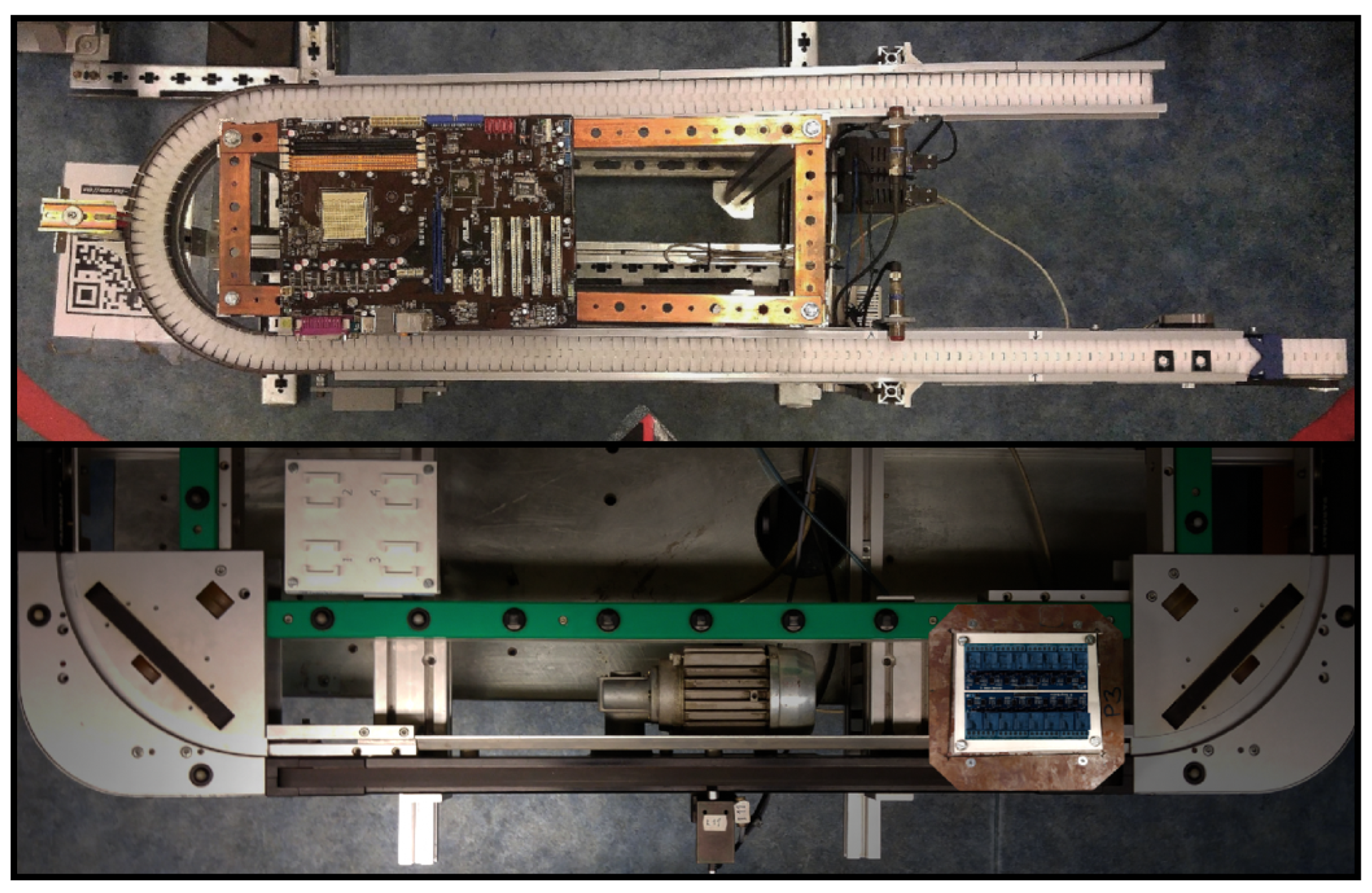
The PCB-based test piece was performed on the Sony SCARA SRX-611 PARO QE 01 31-6000 conveyor (see also Figure 8).
After the above process, a total of 14,576 images became available and captured by the Tapo C200 camera.
The second dataset contains the initial scenes, including classes and the corresponding subregions. We had to take additional steps to create these images.
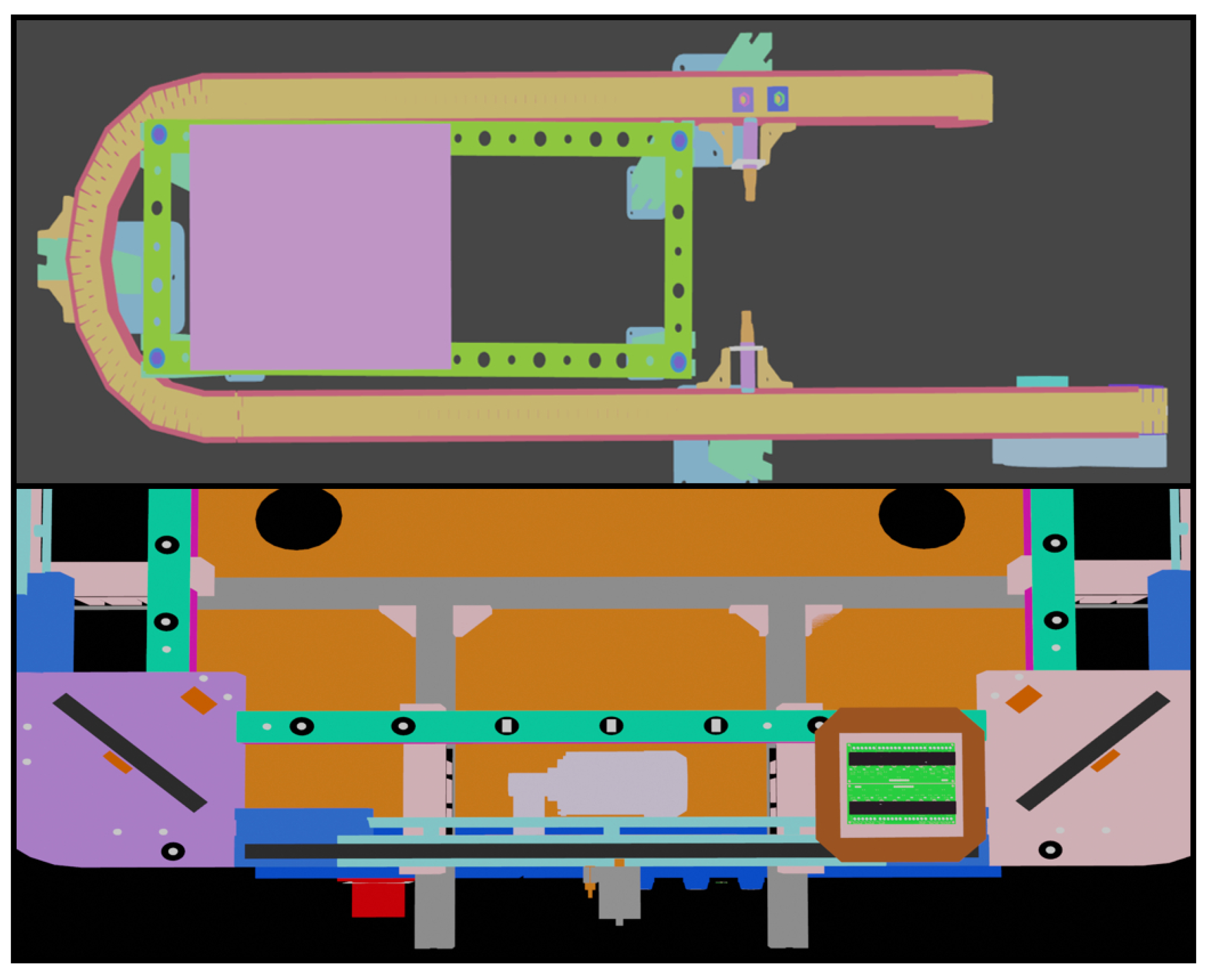
As mentioned earlier, there are two main tasks in designing 3D CAD models of objects moving on an assembly line. One is to actually manufacture the objects using 3D FDM technology, which will be needed for comparison. Once the 3D CAD models are available, the alternative is to produce the element set required for the neural network dataset through digital rendering (see Figure 9).
In our case, the solution was provided by Blender, which is software that is widely used in the industry to perform visualizations and simulations [30]. The program itself is open-source certified (GNU GPL) [31].
We designed 3D CAD models of both Flexlink XK and PARO QE conveyors and then performed polygon reduction on them to reduce the computational demand. We then added a virtual camera to the 3D workspace and virtually guided the test workpieces through the conveyors, rendering them with the same 1080p full HD resolution as the Tapo C200. The rendering was performed using the Cycles engine and a sample voltage of 32 volts (see also Figure 10).
Since it is a 3D CAD model-based rendering, we can produce any number of elements needed for the dataset. As a result, the same 14,576 number of rendered images as for the real images is produced.
The real and generated images are produced in PNG format, as described above, but annotation software is necessary to learn the objects in the images. Therefore, LabelImg [32] was used to achieve this.
First, the photos taken using the real IP camera were annotated using bounding boxes, which were associated with the names of the objects to be recognized (see also Figure 11).
After that, the annotation of the 3D-rendered images was performed. From the RGB color scale, it can be seen that the colors are consistent for rendered images, i.e., they do not contain textures. We now have two datasets for deep-learning-based training.
For annotation and rendering, we used a machine in our lab that is connected to the network. The desktop PC had an Intel Xeon W-2123 CPU (four-core eight-thread), an Nvidia RTX 4060Ti graphics unit, and 64 GB of RAM [33].

5. Architecture Description of the Deep Learning-Based Detector Algorithms

In this section, the architecture of the detectors used to train robot units is described. Several publications are also available on the use of machine learning in real-time operation tasks, which are suitable for industrial applications. Zamora Hernandez et al. described in [34] a visual inspection helper technique based on deep learning and the you only look once (YOLO) architecture. Yu et al. also proposed an effective machine vision-based fault detection process using FPGA acceleration and YOLO V3 architecture-based implementation [35]. Zhou et al. presented an application in which a hybrid architectural solution based on MobileNetv2 and YOLOV4 was considered to improve the accuracy of detecting significantly tiny objects in photos [36]. A. Bochkovskiy et al. improved the YOLO architecture by applying mosaic data augmentation, a new anchor-free detection head, and an improved new loss function [37]. In 2020, another version of YOLO called YOLOv5 was released by the company Ultralytics [38]. As a result, the network architecture has been significantly improved by adding new features such as hyperparameter optimization and integrated experiment tracking. Chien-Yao Wang et al. introduced in [39] a new state-of-the art model based on an approach of trainable bag-of-freebies sets and applying model re-parameterization and scaling techniques to improve the accuracy and speed of their architecture, called YOLOv7. Furthermore, Ultralytics released new YOLO architectures [38,40,41], which introduced new features and improvements for enhanced performance, flexibility, and efficiency and supported a full range of vision AI tasks, including detection, segmentation, pose estimation, tracking, and classification.
Considering the preceding work, we have selected two main YOLO architectures [42,43] for detection since they have very efficient and rapid implementation and can attain a very reasonable level of detection precision.
In the first case, the YOLOv3 detectors can be separated into two major architectural components as follows: the backbone and the detection parts. The backbone block consists of the primary layers, such as the convolution, batch-normalization, MaxPool, and LeakyRELU activation layers, which are responsible for extracting the primary image features. On the other hand, the detection part predicts the object’s bounding box based on the features collected by the backbone block. In our case, we selected the following four distinct architectures for the primary built-in detectors: YOLOV3-tiny, YOLOV3-tiny-3l, YOLOV3-SPP, and YOLOv3-5l. Since our main goal is to verify the operability and accuracy of the detectors, we did not perform any major architectural adjustments; rather, we optimized the detector blocks for the dataset generated through data synthesis. Based on the following equation [37], the number of convolutional layer filters preceding each YOLO layer was determined using the following:
F = 3 · ( D + 5 )
where D denotes the number of detectable classes. Since this will be a single object in our case, substituting it into (5) gives F = 18 layers.
Finally, for each detector, the anchor values were recalculated to achieve the best possible detection accuracy; for this, we used the built-in clustering algorithm, k-means ++ [44]. The values obtained are shown in Table 2.
The loss function of detectors is given as follows (see [43,45]):
l o s s = c l s L o s s + l o c L o s s + c o n f L o s s d + c o n f L o s s m ,
where c l s L o s s denotes the classification, l o s L o s s denotes the localization, and c o n f L o s s d ,   c o n f L o s s m denotes the confidence losses.
In the second case, we have chosen the following four YOLOv8 default detectors depending on the network size and computation demands: YOLOv8-nano, YOLOv8-small, YOLOv8-medium, and YOLOv8-large.
The basic architecture of a network is divided into three parts as follows: the backbone, neck, and head. The backbone block contains the main feature extraction components of the network. The neck part is responsible for connecting the backbone and the head. The last head part generates the final output, and its structure is the same as that of the YOLOv3 detection parts.
Because the network architecture contains several built-in methods and hyperparameter optimization, applying other optimization techniques and methods was not required.

6. Experiments

6.1. Training Details of the Selected Deep Learning-Based Algorithms

In this section, we provide the details of the chosen learning configuration and parameters during the training and evaluation process.

6.1.1. pix2pxHD

The training configuration of the deep learning network that we used for generating the synthesized images were chosen as follows: As an optimizer, the Adam algorithm [46] was used with an initial learning rate of 0.0005, which was left unchanged for the first 40 epochs with a linear decrease afterward. The algorithm was trained over a total number of 200 epochs on 400 image pairs with a resolution of 2048 × 1024 pixels, with a chosen mini-batch size of 16 and without pixel labels, since only the image captures were available. For the rendered images, we created image pairs at the real scene under the lighting conditions typical during operation. We applied only rotation and mirror augmentation during training.

6.1.2. YOLO-Based Detectors

In the first step, we created the initial dataset, which can be divided into the training and validation parts. The training dataset contained 400 images, which were also generated using the selected pix2pixHD algorithm, and the validation part contained only 100 real captured images. In both cases, the resolution of the images was 2048 × 1024.
In cases of YOLOv3, we also applied additional image augmentation algorithms, such as the modification of saturation and exposure, resizing image scenes, and hue shifting [47] to prevent over-training during the learning process. The methods associated with the corresponding parameters are given in Table 3.
After the description of the augmentation process, we selected the Adam method [46] as the appropriate optimizer algorithm. The settings of the momentum and decay parameters of Adam are given in Table 4.
After selecting the optimizer, we had to configure additional learning parameters, such as the initial learning rate, and a scheduler that could provide the proper learning rate values in every epoch. In this case, we choose the exponential scheduler, which is given as follows [48]:
l r = l r initial   exp k #   epochs   ,
where l r initial   is the initial learning rate,   k denotes a hyperparameter value, and epochs will be the number of maximum training iterations. We performed numerous experiments to find the best adjustments for the learning rate and parameter   k . As a result, we have applied a logarithmic search to the parameter domain and obtained the value k = 1 × 10 1 . The best values found for the learning rate are enclosed in Table 3. In the next step, we further configured the learning parameters, such as the maximum epoch value and the burned-in parameter. The burned-in parameter is responsible for providing stability at the beginning of the training process; therefore, it is really important to choose this value properly. In our case, the best value is found to be 100 for each detector. As the last step, we determined the maximum epoch number, which can be expressed as follows [10,37,43]:
E = 2000   ·   D ,
where E denotes the maximum epoch number, and D is the number of classes. In our case, the dataset contained only one detectable object; therefore, that value was 2000.
In the cases of YOLOv8 detectors, we applied the built-in augmentation methods with automatic parameters such as mosaic augmentation and resizing techniques. The corresponding learning parameters, which are applied during training, are given in Table 5.

6.2. Results

This section presents the obtained results of every deep learning-based algorithm with the corresponding metrics, and we also measured the difference between the real and synthetic datasets, which is required for the successful training of the detectors. The algorithms were trained using an Intel Xeon W-2123 CPU (four-core eight-thread), an Nvidia RTX 4060Ti graphics unit, and 64 GB of RAM.
A.
pix2pixHD
The results of the selected pix2pixHD algorithm are given in Table 6 and Table 7. The sampled images obtained during the training process can be seen in Figure 12. The table also contains additional evaluated values with the corresponding standard deviation and the minimum and maximum values at every relevant epoch. We chose a robust algorithm called complex wavelet structural similarity (CWSSIM) [49] because this algorithm is invariant to various transformations, such as rotation and resizing, and is useful in our case. Because of the different sizes of objects and images, some errors can occur in the application of the classical structural similarity method. The intensity and small geometric distortions could also be problem factors. In these cases, we applied minor preprocessing methods to avoid future issues. During the evaluation, we performed histogram equalizations and color corrections. We also included geometric distortion corrections to prevent the main geometric issues. It is important to note that this method can only be applied if the camera matrix and the lens parameters are available.
Therefore, we had to handle and avoid these issues during the evaluation process. The evaluation was applied both to the entire image and to the regions of the objects to be detected. The quality values for the entire image achieved good accuracy at the beginning of the training and the training process reached an acceptable quality, which is already suitable for detection. Consequently, since we will train the detectors based on these regions, they will be the relevant values to obtain the maximum difference between real and synthesized datasets and reach the required image quality and similarity. After computing the standard deviation values and the best and worst results for the dataset, we established that there are minimal deviations for all the images, while we obtained much higher values for the object regions. In the latter case, depending on the proportion of higher- and lower-quality regions, the similarity can significantly affect the accuracy of the detectors during the training process.
B.
YOLO-based detectors
The results of the selected YOLO-based detectors with the corresponding measured quality values (precision, mean average precision, recall, and F1-score) are summarized in Table 8 and Table 9 (mAP50 denotes the average precision up to 0.5 and mAP50–95 denotes the results obtained between 0.5 and 0.95).
As a reference, the detectors were also trained on real images, and the results were given in the first row of the table. In each case, the size of the generated training image dataset consisted of a total of 256,000 images, and the validation dataset contained only 400 real image scenes.
In cases of YOLOv3 detectors, we measured that the accuracy of the detectors decreased significantly in cases in which the structural similarity fell below 0.5. Consequently, we obtained the maximum difference between real and synthesized datasets, which had to be ensured during the training of YOLO-based detector algorithms. During the evaluation, we also established that beginning with a similarity value of at least 0.6, the accuracy of the detectors approaches the results trained on real images. The standard deviation of the object value was also an important factor because if the dataset contained a higher proportion of lower-quality regions, the accuracy of the detectors would be significantly reduced.
In the cases of YOLOv8 detectors, based on the given results, it can be seen that the architecture is more robust than the YOLOv3 detectors. Although the network achieved sufficient accuracy even on low-quality synthetic images, based on the mean average precision, we obtained a similar decrease in accuracy as in the previous case.
Based on the given result, it can be seen easily that the measured similarity affects the precision of training. Suppose the quality level does not meet the minimal requirements after the training of the translation method is finished. In that scenario, the synthesized images significantly deviate from the real ones, making it impossible to train the deep learning algorithms to produce acceptable results.
The reason is that the diversity and content of the initial translation dataset are not adequate. Therefore, we have to improve it by extending various materials and modifying our class regions into new ones.
C.
Real application
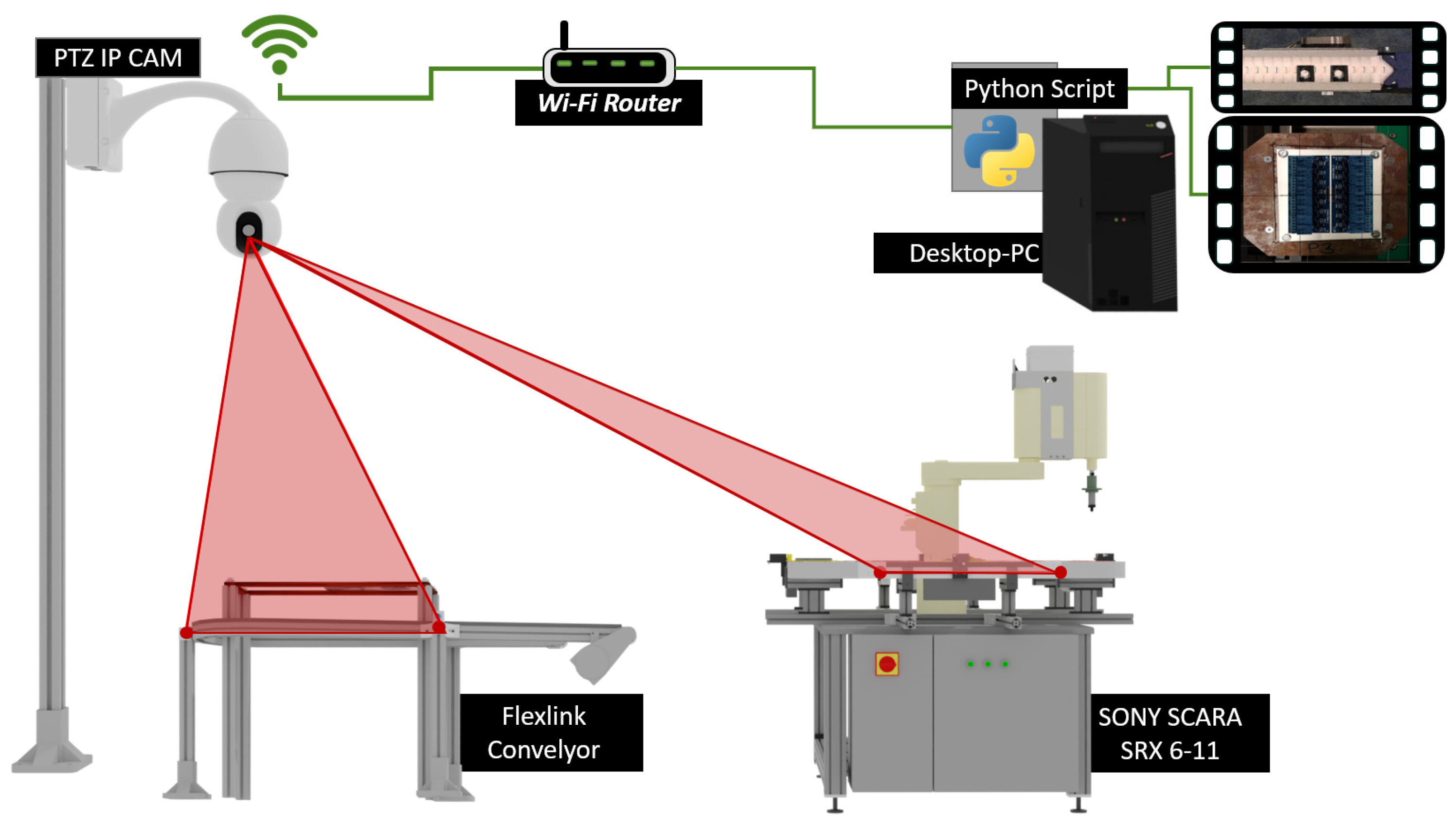
We have also performed real tests with the trained detectors on several devices, such as a desktop PC with an Nvidia RTX 4060Ti GPU card and an Nvidia Jetson Nano development kit [50] and our implemented test environment is shown in Figure 13. It is important to note that industrial machines are not capable of using complex image processing techniques because of hardware limitations.
Figure 13. Layout of our implemented test system. The images are retrieved with a Tapo C200 PTZ IP camera, and the captured scenes are processed using a Python script.
Robotics 13 00088 g013
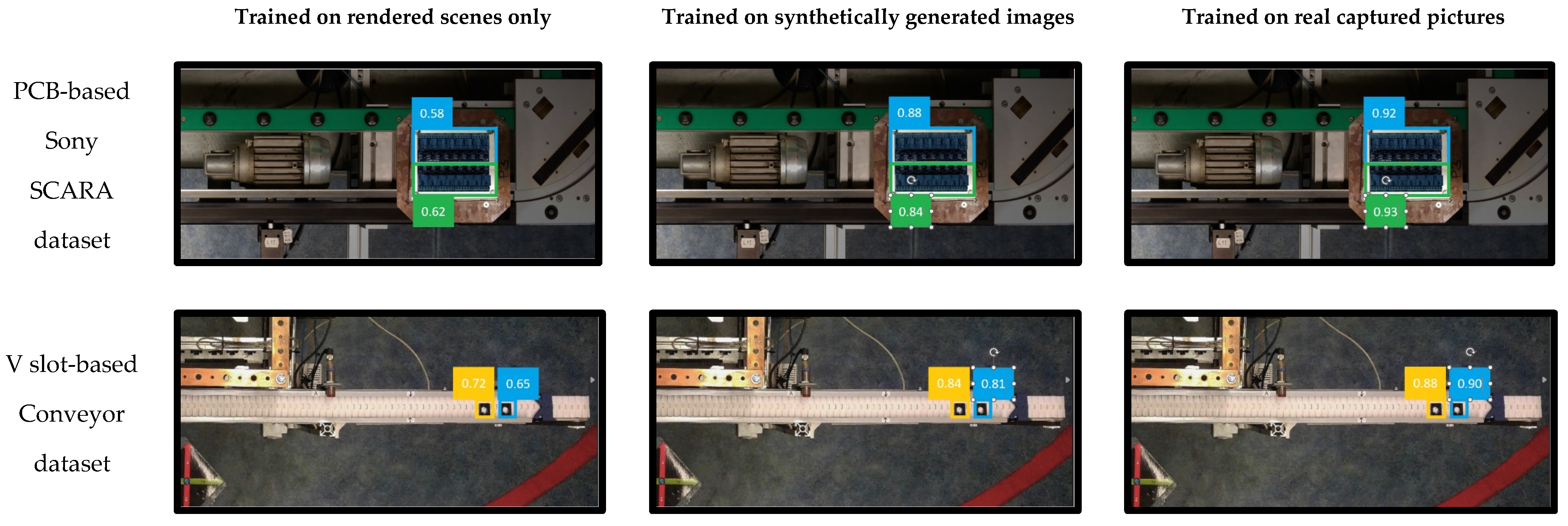
The obtained results according to the different training datasets, are given in Table 10. As detectors for performing tests, we have chosen the following two detectors based on their computing requirements and precision capabilities: YOLOv3-tiny-3l for the conveyor dataset and YOLOv8-nano for the Sony SCARA dataset. Based on the given results, detectors trained on synthetically generated datasets can achieve close to accurate detections as trained on real images (see Figure 14).
During testing, we also measured the inference times on both devices. For YOLOv3-tiny-3l, we obtained about 54.19 milliseconds, and for YOLOv8-nano, we obtained 76.29 milliseconds, which were reasonable results on the Nvidia Jetson device. Performing detectors on a desktop RTX 4060Ti graphical card, we achieved 27.87 and 73.11 milliseconds on average.
Finally, we mention that the proposed dataset translation architecture can also be applied in other cases, such as converting an old image dataset into a new one. Additionally, the texture replacement of objects becomes possible in image scenes. In these cases, three main options are available.
The first is the simplest and fastest solution, but it can only be applied if we can take new pictures with the same camera parameters and settings and if the arrangement of the main objects in the scenes is the same as the previous ones. The borders and sizes of the objects must also be pixel precise. In most cases, this solution is helpful in replacing the materials and lighting conditions on the old dataset images. In the second case, we must take additional steps. If the conditions mentioned in the first option are not met, we have to perform preprocessing to generate train data, including label pixels. The preprocessing can automatically be performed using classical and machine learning algorithms, depending on the complexity of the application area. Several clustering or segmentation algorithms can also be helpful in creating the required label maps to train the data translation method.
In the third case, the preprocessing algorithms can be replaced or combined with handcrafted methods or a manual annotation process to create the class regions. We recommend this solution only if the first two are not applicable and preprocessing does not give accurate results. Additionally, it is essential that the dataset is not too complex or large because of the time-consuming procedures.

7. Conclusions

In this work, training neural networks based on data synthesis was carried out. The data synthesis was implemented using image-to-image translation and 3D modeling. The similarity and quality of the synthesized images were evaluated using the complex wavelet structural similarity metric, and the training of the YOLO detectors was performed based on these values. As a result, we developed an image dataset translation method that applied an image-to-image translation technique to generate new datasets. In metric terms, we reached the quality level, for which the accuracy of detector training approximates that of the reference training. The solution enabled us to apply deep learning-based neural networks to a pre-existing industrial robot unit and the corresponding datasets without completely replacing its control system and at no additional cost.

Author Contributions

T.I.E. and T.P.K. conducted research, established the methodology and designs, and participated in the writing of the paper; G.H. and A.H. conducted the formal analysis and review of the paper. All authors have read and agreed to the published version of the manuscript.

Funding

This research was supported by the TKP2020-NKA-04 project, which has been implemented with the support provided by the National Research, Development, and Innovation Fund of Hungary, financed under the 2020-4.1.1-TKP2020 funding scheme.

Acknowledgments

The authors would like to thank the editor and reviewers for their helpful comments and suggestions, as well as the Doctoral School of Informatics of the University of Debrecen and the Department of Vehicles Engineering of the Faculty of Engineering for infrastructural support. Masuk Abdullah is commended for their invaluable contributions to the development.

Conflicts of Interest

The authors declare no conflicts of interest.

References

  1. Rikalovic, A.; Suzic, N.; Bajic, B.; Piuri, V. Industry 4.0 Implementation Challenges and Opportunities: A Technological Perspective. IEEE Syst. J. 2022, 16, 2797–2810. [Google Scholar] [CrossRef]
  2. Pascal, C.; Raveica, L.-O.; Panescu, D. Robotized application based on deep learning and Internet of Things. In Proceedings of the 2018 22nd International Conference on System Theory, Control and Computing (ICSTCC), Sinaia, Romania, 10 October 2018; pp. 646–651. [Google Scholar] [CrossRef]
  3. Ayub, A.; Wagner, A.R. F-SIOL-310: A Robotic Dataset and Benchmark for Few-Shot Incremental Object Learning. In Proceedings of the 2021 IEEE International Conference on Robotics and Automation (ICRA), Xi’an, China, 30 May–5 June 2021; pp. 13496–13502. [Google Scholar] [CrossRef]
  4. Jiang, P.; Ishihara, Y.; Sugiyama, N.; Oaki, J.; Tokura, S.; Sugahara, A.; Ogawa, A. Depth Image–Based Deep Learning of Grasp Planning for Textureless Planar-Faced Objects in Vision-Guided Robotic Bin-Picking. Sensors 2020, 20, 706. [Google Scholar] [CrossRef] [PubMed]
  5. Lobbezoo, A.; Qian, Y.; Kwon, H.-J. Reinforcement Learning for Pick and Place Operations in Robotics: A Survey. Robotics 2021, 10, 105. [Google Scholar] [CrossRef]
  6. Sumanas, M.; Petronis, A.; Bucinskas, V.; Dzedzickis, A.; Virzonis, D.; Morkvenaite Vilkonciene, I. Deep Q-Learning in Robotics: Improvement of Accuracy and Repeatability. Sensors 2022, 22, 3911. [Google Scholar] [CrossRef]
  7. Imad, M.; Doukhi, O.; Lee, D.J.; Kim, J.C.; Kim, Y.J. Deep Learning-Based NMPC for Local Motion Planning of Last-Mile Delivery Robot. Sensors 2022, 22, 8101. [Google Scholar] [CrossRef] [PubMed]
  8. KUKA Robotics, Official Documentation of Industrial ARC Welder Robot Arm. Available online: https://www.eurobots.net/robot_kuka_kr5_arc-en.html (accessed on 1 May 2023).
  9. SONY SCARA SRX—11; High-Speed Assembly Robot, Operation Manual. SONY Corporation: Tokyo, Japan, 1996.
  10. Kapusi, T.P.; Erdei, T.I.; Husi, G.; Hajdu, A. Application of deep learning in the deployment of an industrial scara machine for real-time object detection. Robotics 2022, 11, 69. [Google Scholar] [CrossRef]
  11. Bajda, M.; Hardygóra, M.; Marasová, D. Energy Efficiency of Conveyor Belts in Raw Materials Industry. Energies 2022, 15, 3080. [Google Scholar] [CrossRef]
  12. Stepper Motor, ST5918L4508-B—STEPPER MOTOR—NEMA 23. Available online: https://en.nanotec.com/products/537-st5918l4508-b (accessed on 22 January 2023).
  13. PARO QE 01 31-6000; Manual of the Modular Conveyor. PARO AG: Subingen, Switzerland, 2016.
  14. Hullin, M.; Eisemann, E.; Seidel, H.-P.; Lee, S. Physically-based real-time lens flare rendering. ACM Trans. Graph. 2011, 30, 108. [Google Scholar] [CrossRef]
  15. Lee, S.; Eisemann, E. Practical real-time lens-flare rendering. Comput. Graph. Forum 2013, 32, 1–6. [Google Scholar] [CrossRef]
  16. Seland, D. An industry demanding more: Intelligent illumination and expansive measurement volume sets the new helix apart from other 3-d metrology solutions. Quality 2011, 50, 22–24. Available online: https://link.gale.com/apps/doc/A264581412/AONE (accessed on 25 August 2023).
  17. Martinez, P.; Ahmad, D.R.; Al-Hussein, M. A vision-based system for pre-inspection of steel frame manufacturing. Autom. Constr. 2019, 97, 151–163. [Google Scholar] [CrossRef]
  18. Wu, Y.; He, Q.; Xue, T.; Garg, R.; Chen, J.; Veeraraghavan, A.; Barron, J.T. How to Train Neural Networks for Flare Removal. In Proceedings of the IEEE/CVF International Conference on Computer Vision (ICCV), Montreal, QC, Canada, 17 October 2021; pp. 2239–2247. [Google Scholar]
  19. Chen, S.-T.; Cornelius, C.; Martin, J.; Chau, D.H. Robust Physical Adversarial Attack on Faster R-CNN Object Detector. arXiv 2018, arXiv:1804.05810. [Google Scholar]
  20. Kapusi, T.P.; Kovacs, L.; Hajdu, A. Deep learning-based anomaly detection for imaging in autonomous vehicles. In Proceedings of the 2022 IEEE 2nd Conference on Information Technology and Data Science (CITDS), Debrecen, Hungary, 16–18 May 2022; pp. 142–147. [Google Scholar]
  21. Branytskyi, V.; Golovianko, M.; Malyk, D.; Terziyan, V. Generative adversarial networks with bio-inspired primary visual cortex for industry 4.0 Procedia Computer. Science 2022, 200, 418–427. [Google Scholar] [CrossRef]
  22. Mei, S.; Yudan, W.; Wen, G. Automatic fabric defect detection with a multi-scale convolutional denoising autoencoder network model. Sensors 2018, 18, 1064. [Google Scholar] [CrossRef] [PubMed]
  23. Kaji, S.; Kida, S. Overview of image-to-image translation by use of deep neural networks: Denoising, super-resolution, modality conversion, and reconstruction in medical imaging. Radiol. Phys. Technol. 2019, 12, 235–248. [Google Scholar] [CrossRef] [PubMed]
  24. Wang, T.-C.; Liu, M.-Y.; Zhu, J.-Y.; Tao, A.; Kautz, J.; Catanzaro, B. High-resolution image synthesis and semantic manipulation with con- ditional gans. In Proceedings of the IEEE Conference on Computer Vision and Pattern Recognition, Salt Lake City, UT, USA, 18–22 June 2018; pp. 8798–8807. [Google Scholar]
  25. Zhu, J.-Y.; Park, T.; Isola, P.; Efros, A.A. Unpaired image-to-image translation using cycle-consistent adversarial networks. In Proceedings of the IEEE International Conference on Computer Vision (ICCV), Venice, Italy, 22–29 October 2017. [Google Scholar]
  26. Andreucci, C.A.; Fonseca, E.M.M.; Jorge, R.N. 3D Printing as an Efficient Way to Prototype and Develop Dental Implants. BioMedInformatics 2022, 2, 671–679. [Google Scholar] [CrossRef]
  27. Korol, M.; Vanca, J.; Majstorovic, V.; Kocisko, M.; Baron, P.; Torok, J.; Vodilka, A.; Hlavata, S. Study of the Influence of Input Parameters on the Quality of Additively Produced Plastic Components. In Proceedings of the 2022 13th International Conference on Mechanical and Aerospace Engineering (ICMAE), Bratislava, Slovakia, 20 July 2022; pp. 39–44. [Google Scholar] [CrossRef]
  28. Engineers EDGE, “ABS Plastic Filament Engineering Information”. Available online: https://www.engineersedge.com/3D_Printing/abs_plastic_filament_engineering_information_14211.htm (accessed on 12 October 2023).
  29. Chatzoglou, E.; Kambourakis, G.; Smiliotopoulos, C. Let the Cat out of the Bag: Popular Android IoT Apps under Security Scrutiny. Sensors 2022, 22, 513. [Google Scholar] [CrossRef] [PubMed]
  30. Du, Y.; Sun, H.Q.; Tian, Q.; Zhang, S.Y.; Wang, C. Design of blender IMC control system based on simple recurrent networks. In Proceedings of the 2009 International Conference on Machine Learning and Cybernetics, Baoding, China, 12 July 2009; pp. 1048–1052. [Google Scholar] [CrossRef]
  31. Takala, T.M.; Mäkäräinen, M.; Hamalainen, P. Immersive 3D modeling with Blender and off-the-shelf hardware. In Proceedings of the Conference: 3D User Interfaces (3DUI), 2013 IEEE Symposium, Orlando, FL, USA, 16–17 March 2013. [Google Scholar]
  32. Li, J.; Meng, L.; Yang, B.; Tao, C.; Li, L.; Zhang, W. LabelRS: An Automated Toolbox to Make Deep Learning Samples from Remote Sensing Images. Remote Sens. 2021, 13, 2064. [Google Scholar] [CrossRef]
  33. Lenovo. ThinkCentre M93 Tower. Available online: https://www.lenovo.com/hu/hu/desktops/thinkcentre/m-series-towers/ThinkCentre-M93P/p/11TC1TMM93P (accessed on 2 October 2022).
  34. Zamora, M.; Vargas, J.A.C.; Azorin-Lopez, J.; Rodr’ıguez, J. Deep learning-based visual control assistant for assembly in industry 4.0. Comput. Ind. 2021, 131, 103485. [Google Scholar] [CrossRef]
  35. Yu, L.; Zhu, J.; Zhao, Q.; Wang, Z. An efficient yolo algorithm with an attention mechanism for vision-based defect inspection deployed on FPGA. Micromachines 2022, 13, 1058. [Google Scholar] [CrossRef]
  36. Zhou, X.; Xu, X.; Liang, W.; Zeng, Z.; Shimizu, S.; Yang, L.T.; Jin, Q. Intelligent small object detection for digital twin in smart manufacturing with industrial cyber-physical systems. IEEE Trans. Ind. Inform. 2022, 18, 1377–1386. [Google Scholar] [CrossRef]
  37. Bochkovskiy, A.; Wang, C.; Liao, H.M. Yolov4: Optimal speed and accuracy of object detection. arXiv 2020, arXiv:2004.10934. Available online: https://arxiv.org/abs/2004.10934 (accessed on 30 July 2023).
  38. Gašparović, B.; Mauša, G.; Rukavina, J.; Lerga, J. Evaluating YOLOV5, YOLOV6, YOLOV7, and YOLOV8 in Underwater Environment: Is There Real Improvement? In Proceedings of the 2023 8th International Conference on Smart and Sustainable Technologies (SpliTech), Split/Bol, Croatia, 20–23 June 2023; pp. 1–4. [Google Scholar] [CrossRef]
  39. Wang, C.-Y.; Bochkovskiy, A.; Liao, H.-Y.M. YOLOv7: Trainable Bag-of-Freebies Sets New State-of-the-Art for Real-Time Object Detectors. In Proceedings of the 2023 IEEE/CVF Conference on Computer Vision and Pattern Recognition (CVPR), Vancouver, BC, Canada, 17–24 June 2023; pp. 7464–7475. [Google Scholar] [CrossRef]
  40. Afdhal, A.; Saddami, K.; Sugiarto, S.; Fuadi, Z.; Nasaruddin, N. Real-Time Object Detection Performance of YOLOv8 Models for Self-Driving Cars in a Mixed Traffic Environment. In Proceedings of the 2023 2nd International Conference on Computer System, Information Technology, and Electrical Engineering (COSITE), Banda Aceh, Indonesia, 2 August 2023; pp. 260–265. [Google Scholar] [CrossRef]
  41. Wang, C.Y.; Yeh, I.H.; Liao, H.Y. YOLOv9: Learning What You Want to Learn Using Programmable Gradient Information. arXiv 2024, arXiv:2402.13616. Available online: https://arxiv.org/abs/2402.13616 (accessed on 20 March 2024).
  42. Adarsh, P.; Rathi, P.; Kumar, M. Yolo v3-tiny: Object detection and recognition using one stage improved model. In Proceedings of the 2020 6th international conference on advanced computing and communication systems (ICACCS), Coimbatore, India, 6–7 March 2020; pp. 687–694. [Google Scholar]
  43. Redmon, J.; Farhadi, A. Yolov3: An incremental improvement. arXiv 2018, arXiv:1804.02767. Available online: http://arxiv.org/abs/1804.02767 (accessed on 2 August 2023).
  44. Arthur, D.; Vassilvitskii, S. K-means++: The advantages of careful seeding. Soda 2007, 8, 1027–1035. [Google Scholar]
  45. Redmon, J.; Divvala, S.; Girshick, R.; Farhadi, A. You only look once: Unified, real-time object detection. In Proceedings of the IEEE Conference on Computer Vision and Pattern Recognition, Las Vegas, Nevada, USA, 27–30 June 2016; pp. 779–788. [Google Scholar]
  46. Kingma, D.P.; Ba, J. Adam: A method for stochastic optimization. arXiv 2014, arXiv:1412.6980. Available online: https://arxiv.org/abs/1412.6980 (accessed on 2 August 2023).
  47. Perez, L.; Wang, J. The effectiveness of data augmentation in image classification using deep learning. arXiv 2017, arXiv:1712.04621. Available online: http://arxiv.org/abs/1712.04621 (accessed on 25 August 2023).
  48. Li, Z.; Arora, S. An exponential learning rate schedule for deep learning. arXiv 2019, arXiv:1910.07454. Available online: http://arxiv.org/abs/1910.07454 (accessed on 3 August 2023).
  49. Sampat, M.P.; Wang, Z.; Gupta, S.; Bovik, A.C.; Markey, M.K. Complex wavelet structural similarity: A new image similarity index. IEEE Trans. Image Process. 2009, 18, 2385–2401. [Google Scholar] [CrossRef]
  50. Nvidia Jetson Nano Developer Kit. 2024. Available online: https://developer.nvidia.com/embedded/jetson-nano-developer-kit (accessed on 9 December 2023).
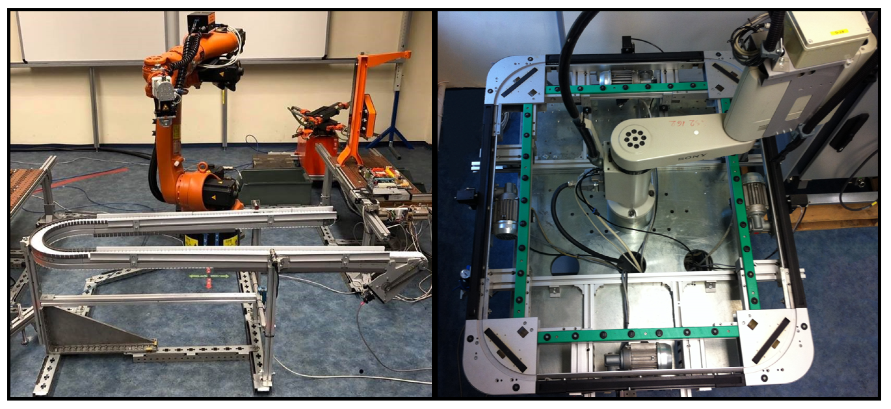
Figure 1. KUKA KKR5 Flexlink XK and Sony SCARA SRX-611 PARO QE 01 31-6000.
Robotics 13 00088 g001
Figure 2. Components of real image descriptiveness.
Robotics 13 00088 g002
Figure 3. Architecture of dataset translation method.
Robotics 13 00088 g003
Figure 4. Translation of the images.
Robotics 13 00088 g004
Figure 5. In-house-developed FDM 3D printer.
Robotics 13 00088 g005
Figure 6. Layer and speed view of objects.
Robotics 13 00088 g006
Figure 8. Workpieces on Flexlink XK and PARO QE conveyors.
Robotics 13 00088 g008
Figure 9. Creating a synthesized dataset.
Robotics 13 00088 g009
Figure 10. 3D CAD-based image rendering.
Robotics 13 00088 g010
Figure 11. Annotations of the real images.
Robotics 13 00088 g011
Figure 12. Outputs of synthesized image scenes during the training of the pix2pixHD algorithm.
Robotics 13 00088 g012
Figure 14. Some results of the tested detectors.
Robotics 13 00088 g014
Table 1. Parameters of ABS filament [28].
PropertyAcrylonitrile Butadiene Styrene (ABS)
Density p (Mg/m3)1.00–1.22
Young’s Modulus E (GPa)1.12–2.87
Elongation at break (%)3–75
Melting (softening) Temperature (°C)88–128
Glass Transition Temperature (°C)100
Ultimate Tensile Strength (MPa)33–110
Table 2. Newly computed anchor values.
AnchorYOLOV3-TinyYOLOV3-tini-3lYOLOV3-SPPYOLOV3-5l
010 × 912 × 712 × 710 × 6
113 × 89 × 109 × 1010 × 10
210 × 1010 × 1010 × 109 × 10
311 × 1011 × 1011 × 1010 × 10
412 × 1011 × 1011 × 1010 × 10
514 × 1011 × 1011 × 1011 × 10
6-13 × 1013 × 1011 × 10
7-14 × 914 × 911 × 10
8-15 × 1115 × 1113 × 8
9---12 × 10
10---11 × 10
11---12 × 10
12 13 × 10
13 14 × 10
14 15 × 12
Table 3. Applied image augmentation algorithms and their parameter settings.
Algorithm NameParameter Value
Saturation1.5
Exposure1.5
Resizing1.5
Hue shifting0.3
Table 4. Learning parameters of the YOLOv3-based detectors.
Detector TypeLearning RateMomentumDecay
YOLOV3-tiny0.0050.90.0005
YOLOV3-tiny-3l0.00050.90.0005
YOLOV3-SPP0.00030.90.0005
Table 5. Learning parameters of the YOLOv8-based detectors.
Parameter NameValue
initial learning rate0.01
final learning rate0.001
momentum0.937
weight_decay0.0005
warmup_epochs3.0
warmup_momentum0.8
warmup_bias_learning rate0.1
Table 6. Quality results of the pix2pixhd algorithm based on the conveyor dataset.
Epochs C W S S I M I m a g e ¯ σ C W S S I M I m a g e m i n C W S S I M I m a g e m a x C W S S I M I m a g e C W S S I M o b j ¯ σ C W S S I M o b j m i n C W S S I M o b j m a x C W S S I M o b j
10.61349.5687 × 10−50.61110.61560.38450.03470.12450.6289
20.68269.2365 × 10−40.68060.68430.40050.05480.18690.6902
30.72548.9854 × 10−40.72240.72790.42540.06540.21430.7216
40.73899.7564 × 10−40.73680.73970.44930.04580.21100.7304
50.78268.7052 × 10−40.78140.78430.46470.05990.24040.7477
60.80538.9652 × 10−40.80340.80640.48860.03210.23120.7507
70.81157.4652 × 10−40.81030.81310.49310.02450.24080.7633
80.81497.3254 × 10−40.81210.81570.50260.04580.26550.7707
90.82046.7478 × 10−40.81940.82120.49160.05010.28870.7798
100.83497.6548 × 10−40.83240.83610.51340.05460.32470.7925
200.83536.2248 × 10−40.83310.83690.54950.04960.33350.7811
300.84696.0654 × 10−40.84470.84830.57660.05120.34690.7761
400.85795.6335 × 10−40.85600.85910.60240.05640.35040.7848
500.86224.4256 × 10−40.86030.86340.58890.05240.34750.7991
600.86765.2145 × 10−40.86580.86890.61240.05300.36640.7948
700.87065.0125 × 10−40.86920.87140.60650.05350.35860.7890
800.87654.7879 × 10−40.87510.87830.62480.05090.34960.8122
900.87894.4578 × 10−40.87620.87980.64240.04960.37890.8046
1000.87954.1254 × 10−40.87740.89090.63490.05240.38640.7899
1400.88023.8878 × 10−40.87890.88140.64010.05960.39410.7943
2000.88153.7998 × 10−40.88010.88320.65780.05520.42290.7873
Table 7. Quality results of the pix2pixhd algorithm based on the Sony SCARA dataset.
epochs C W S S I M I m a g e ¯ σ C W S S I M I m a g e m i n C W S S I M I m a g e m a x C W S S I M I m a g e C W S S I M o b j ¯ σ C W S S I M o b j m i n C W S S I M o b j m a x C W S S I M o b j
10.75424.2548× 10−30.75140.75860.43480.06010.36210.5408
20.79453.9547× 10−30.79260.79140.49630.05690.40900.6140
30.80023.6985× 10−30.79750.80420.52690.03540.43560.6432
40.82392.9645× 10−30.82100.82510.50480.04870.45410.6892
50.84772.4123× 10−40.84530.84900.53690.03690.48020.7013
60.89142.2658× 10−40.89020.89320.60870.05780.54020.7274
70.90011.5478 × 10−30.89820.90240.63960.04690.55040.7364
80.90571.9625 × 10−40.90340.90760.68960.03980.56660.7559
90.91111.4785 × 10−40.90990.91270.70690.03520.58690.7624
100.91599.6582 × 10−40.91350.91670.68740.02450.57640.7318
200.92097.6584 × 10−40.91880.92130.73690.02690.61450.8236
300.92386.1458 × 10−40.92200.92510.78460.02100.69520.8735
400.92936.6548 × 10−40.92870.93100.75690.02890.68400.8833
500.93595.2145 × 10−40.93400.93720.82470.03690.72480.9103
600.94485.9658 × 10−40.94230.94650.85690.02030.78650.9245
700.95065.4568 × 10−40.94850.95160.87400.03260.82490.9143
800.95485.1254 × 10−40.95340.95620.86740.03540.83410.9354
900.96274.9854 × 10−40.96040.96450.89900.04980.85170.9366
1000.96814.2458 × 10−40.96690.96980.90690.02830.87240.9449
1400.97065.3200 × 10−40.96920.97100.91870.03230.88440.9504
2000.97276.1205 × 10−40.97090.97440.92690.02950.89970.9569
Table 8. Results obtained by the detector for synthesized image quality based on the conveyor dataset.
C W S S I M o b j ¯ YOLOV3-TinyYOLOv3-Tiny-3lYOLOv3-SPPYOLOv3-5l
mAPPrec.RecallF1-ScoremAPPrec.RecallF1-ScoremAPPrec.RecallF1-ScoremAPPrec.RecallF1-Score
1.0000.90650.910.900.910.84680.850.870.860.87780.890.850.870.92961.000.940.96
0.38450.31450.440.250.290.12210.030.000.000.39490.420.400.480.45010.550.200.33
0.40050.36980.490.260.350.14690.260.080.150.42110.490.450.500.50680.670.290.46
0.42540.38460.520.220.340.39860.410.240.340.48010.520.470.490.56980.750.380.54
0.49310.48650.580.350.450.44250.560.350.410.52590.560.540.550.64210.810.510.67
0.50260.54690.620.560.600.56850.600.480.520.54580.630.510.610.72480.860.690.71
0.51340.56940.760.620.690.60480.650.540.580.68460.710.680.690.86940.890.720.79
0.54950.64850.780.730.750.63810.670.620.630.79540.810.780.790.88960.920.760.83
0.64010.80690.840.810.820.79540.810.770.780.83050.850.820.840.910.960.840.91
Table 9. Results obtained by the detector for synthesized image quality based on Sony SCARA dataset.
C W S S I M o b j ¯ YOLOv8-NanoYOLOv8-SmallYOLOv8-MediumYOLOv8-Large
Prec.RecallmAP50mAP50–95 Prec.RecallmAP50mAP50–95Prec.RecallmAP50mAP50–95Prec.RecallmAP50mAP50–95
1.000.9991.0000.9950.8350.9991.0000.9950.8430.9991.0000.9950.8360.9981.0000.9950.845
0.43480.89700.7200.7230.5430.8930.6510.7050.5510.7340.7100.7280.4550.8710.4430.6910.433
0.49630.88000.8600.8840.6130.8960.7750.7310.6670.7780.7590.7960.6530.7790.5250.7100.607
0.52690.88600.9020.8460.6580.8960.8950.7640.6990.8480.7930.8360.7350.8600.7460.7400.681
0.63960.89801.0000.8960.7120.9280.9900.8250.7460.8890.8900.8820.7450.9270.8470.8840.703
0.68960.92601.0000.9120.7360.9511.0000.8950.7660.9480.9400.9050.7860.9680.9550.8950.743
0.68740.91801.0000.9230.7420.9981.0000.9010.8120.9980.9800.9440.7970.9890.9790.9250.784
0.73690.98801.0000.9790.7860.9971.0000.9950.8290.9980.9900.9890.8190.9921.0000.9850.802
0.91870.99801.0000.9910.8020.9981.0000.9950.8350.9981.0000.9950.8270.9981.0000.9950.814
Table 10. Detection results regarding the different training datasets.
Training DatasetConveyor DatasetSony SCARA Dataset
TrainValTestTrainValTest
Rendered only0.6240.6120.5110.6890.6740.655
Synthetic image translation generated0.7950.7840.7780.8020.7820.775
Real images0.8470.8230.8140.8350.8220.802
Disclaimer/Publisher’s Note: The statements, opinions and data contained in all publications are solely those of the individual author(s) and contributor(s) and not of MDPI and/or the editor(s). MDPI and/or the editor(s) disclaim responsibility for any injury to people or property resulting from any ideas, methods, instructions or products referred to in the content.