Article

Evaluating the Performance of Mobile-Convolutional Neural Networks for Spatial and Temporal Human Action Recognition Analysis

by
Stavros N. Moutsis
*,
Konstantinos A. Tsintotas
,
Ioannis Kansizoglou
and
Antonios Gasteratos
Department of Production and Management Engineering, Democritus University of Thrace, 12 Vas. Sophias, GR-671 32 Xanthi, Greece
*
Author to whom correspondence should be addressed.
Robotics 2023, 12(6), 167; https://doi.org/10.3390/robotics12060167
Submission received: 27 September 2023 / Revised: 28 November 2023 / Accepted: 5 December 2023 / Published: 8 December 2023
(This article belongs to the Special Issue Towards Socially Intelligent Robots)

Abstract

:
Human action recognition is a computer vision task that identifies how a person or a group acts on a video sequence. Various methods that rely on deep-learning techniques, such as two- or three-dimensional convolutional neural networks (2D-CNNs, 3D-CNNs), recurrent neural networks (RNNs), and vision transformers (ViT), have been proposed to address this problem over the years. Motivated by the fact that most of the used CNNs in human action recognition present high complexity, and the necessity of implementations on mobile platforms that are characterized by restricted computational resources, in this article, we conduct an extensive evaluation protocol over the performance metrics of five lightweight architectures. In particular, we examine how these mobile-oriented CNNs (viz., ShuffleNet-v2, EfficientNet-b0, MobileNet-v3, and GhostNet) execute in spatial analysis compared to a recent tiny ViT, namely EVA-02-Ti, and a higher computational model, ResNet-50. Our models, previously trained on ImageNet and BU101, are measured for their classification accuracy on HMDB51, UCF101, and six classes of the NTU dataset. The average and max scores, as well as the voting approaches, are generated through three and fifteen RGB frames of each video, while two different rates for the dropout layers were assessed during the training. Last, a temporal analysis via multiple types of RNNs that employ features extracted by the trained networks is examined. Our results reveal that EfficientNet-b0 and EVA-02-Ti surpass the other mobile-CNNs, achieving comparable or superior performance to ResNet-50.

1. Introduction

Human action (or activity) recognition attempts to determine what action is being performed by an individual or a group in a video sequence [1]. Even if this can be considered a simple task, it has puzzled computer vision scholars for several decades [2,3,4]. Throughout this period, human action recognition has been widely adopted by various scientific fields, such as human–machine interaction [5,6], medical assistive technologies [7,8,9,10], surveillance systems [11,12], sports analysis [13], and human–robot interaction [14,15]. Similarly, it assists in path planning for tasks like social collision avoidance and route optimization [16] in autonomous navigation [17]. However, the main reasons why human action recognition constitutes such a challenging task are the following. The first concerns the environment where the action occurs: entirely different surroundings may present the same act. Additionally, the direction might vary from one video to another (e.g., a person walks from right to left and vice versa). The second challenge is related to the sensor’s position, which affects the recorded visual information. More specifically, the closer the sensor is to the scene, the more detailed information it provides, yet the more negligible the action it covers. Moreover, the video streams recorded by a steady camera should be perfectly stabilized; otherwise, the motion adds extra noise to the incoming data. To this end, the large amount of data needed is a common barrier to efficient solutions. Last is the curse of dimensionality: video sequences used for human action recognition use more than 500 image-frames with similar information, enlarging the size of the datasets.
Nevertheless, several methods have been proposed to address this problem based on different data types and techniques, which are mainly distinguished into two categories [18]. The first regards pipelines that apply representation-based solutions, such as global [18,19,20], local [18,19,21,22], and depth [23,24] ones. On the other hand, techniques of the second category concern frameworks implemented with deep-network-based pipelines, such as convolutional neural networks (CNNs) [25]. Despite the promising results of the former systems, their need to adapt to changes (e.g., environmental, frame background, or camera motion) between videos containing the same action presents a disadvantage. In contrast, the latter can adjust to the above challenges, showing remarkable outcomes in different computer vision and robotics tasks [26] (e.g., image recognition [27], object detection [28,29], visual-based navigation [30,31], place recognition [32,33,34], loop closure detection [35,36], and video description [37]). In particular, these approaches use two-dimensional CNNs (2D-CNNs) that receive a grid of values as input (i.e., an image) and subsequently perform spatial analysis via 2D convolutional filters. This way, they keep most of the image’s information while reducing its dimensionality [38]. To this end, many CNN architectures have been proposed in the previous years, reaching improved performances (viz., LeNet [39], AlexNet [40], GoogleNet or InceptionNet [41], BN-Inception [42], VGGNet [27], and ResNet [43]). Still, many trainable parameters are retained in these models, rendering their training process time consuming (i.e., more than a week when employed on ImageNet [44,45]), even if modern graphics processing units (GPUs) are used. Because of this, mobile-CNNs (viz., YOLO [28], MobileNet-v1 [46], MobileNet-v2 [47], ShuffleNet-v1 [48], SuffleNet-v2 [49], NASNetMobile [50], FBNet [51], EfficientNet-b0 [52], MobileNet-v3 [53], and GhostNet [54]) were designed with fewer trainable parameters, simultaneously maintaining high outputs. In most of the cases, when 2D-CNNs are employed for human action recognition, these are large architectures [55], such as CNN-M-2048 [56,57,58], which is similar to ClarifaiNet [59], AlexNet [60], VGGNet [61,62,63], ResNet [64,65], GoogleNet [57], and BN-Inception [61,66]. When mobile versions are used, these include MobileNet-v2 [55,67] and EfficientNet-b0 [68]. Vision transformers (ViT) [69], which were recently introduced for different computer vision tasks (such as image classification [70], object detection [71], image segmentation [72], and action recognition [73,74,75], were inspired by their success in natural language processing [76]. However, while they show dominance over CNNs [77,78], they are characterized by high-complexity models in accordance with their demands for large-scale datasets [69,79]. On the contrary, lightweight models, such as Swin-T [80], MobileViT [81], and EVA-02-Ti [82], have also been applied, showing high performances.
Although deep learning techniques reach high accuracy scores, networks based on many parameters and floating point operations per second (FLOPs) are computationally costly. Due to this fact, since roboticists primarily experiment with mobile platforms, mainly characterized by restricted computational powers, lightweight frameworks are deemed more suitable [83]. To this end, architectures presenting high complexity during inference are unsuitable, as they increase the latency and decrease the power autonomy of the system. Given the abovementioned considerations and the fact that lightweight 2D-CNNs show limited adoption in action recognition tasks [55], in this work, we implement an extensive evaluation protocol over the performance of four mobile-CNNs, namely ShuffleNet-v2, EfficientNet-b0, MobileNet-v3, and GhostNet, and the EVA-02-Ti lightweight vision transformer. A comparison is also performed against ResNet-50, aiming for this work to be self-contained. Our experiments took place on HDB51 [84], UCF101 [85], and NTU [86,87], which are three widely used and known datasets. Our evaluation is based on the deep learning models’ performance according to their average and max scores, as well as their voting, by applying two sampled frame types for each video. It is worth noting that temporal analysis is also provided as the activity’s information is derived from a sequence of consecutive images. Hence, we use the selected neural networks as feature extractors, which are subsequently utilized for recurrent neural networks’ (RNNs) training and testing. This way, we present a holistic evaluation protocol for spatial and temporal human action recognition analysis to help future robotics scholars decide which mobile NN executes better according to the application required.
The main contributions of the proposed study are summarized as follows:
  • Since most of the literature referred to high-complexity networks, our article implements an extended performance evaluation on four mobile and widely used CNNs and a tiny ViT for human action recognition with three datasets. At the same time, for the sake of completeness, a non-lightweight CNN is also tested.
  • With regard to models’ evaluation, the examination is based on the following points:
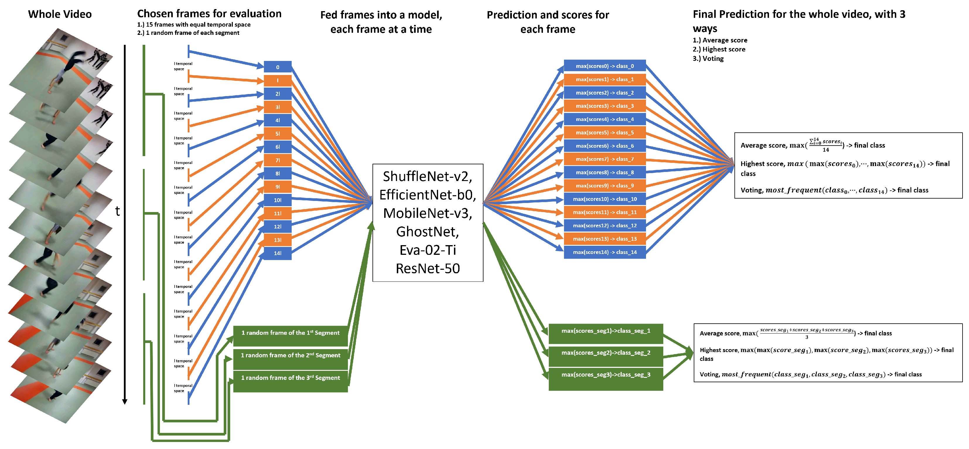
    Nine for the spatial analysis:
    *
    The rate of the dropout layer at p = 0.8 and p = 0.5 .
    *
    The previous models’ training on ImageNet and ImageNet + BU101.
    *
    The final prediction according to the average/max/voting score of 15 and 3 frames.
    Six for the temporal analysis:
    *
    Classification based on all 15 outputs of RNN, long short-term memory (LSTM), and gated recurrent unit (GRU).
    *
    Classification based on the last output of RNN/LSTM/GRU.
  • This work extensively evaluates known resource-efficient models and techniques in activity recognition. Our comprehensive approach can assist researchers in choosing suitable architectures, highlighting lightweight networks and techniques based on performance across three diverse datasets.
The remainder of this article is organized as follows. Section 2 briefly reviews approaches addressing human action recognition based on deep learning. Section 3 describes the selected neural networks, datasets, and applied techniques, and it gives the implementation details, including the training and testing protocols. Section 4 and Section 5 present our results, and Section 6 presents a discussion of those results. Finally, the last section provides the conclusions.

2. Related Work

When tackling human action recognition, 2D-CNN models usually perform spatial analysis on the incoming RGB image frames. In addition, various algorithms are employed to accomplish the temporal analysis. The following section briefly describes these approaches, aiming to present the reader with the state-of-the-art solutions. In particular, pipelines based on 3D-CNNs, two-stream CNNs, temporal segment networks, and CNN + RNN are explored.

2.1. Human Action Recognition through 3D-CNNs

As 3D convolutional filters can be applied to a sequence of consecutive images, performing spatial and temporal analysis simultaneously, 3D-CNNs have been proposed for human action recognition. Using a set of such models and capturing the video’s visual appearance and motion dynamics, the authors in [88] propose a framework where the final prediction results from all the used models. Their pipeline is based on several architectures, giving better outcomes for different datasets. Nevertheless, they mention drawbacks, such as the high complexity and computational cost. Aiming to tackle this weakness, Sun et al. [89] simulate the 3D-CNN function utilizing 2D kernels at the first layers for spatial analysis, with 1D kernels following for the temporal analysis. Combined with improved dense trajectories (iDT) [21] and a linear support vector machine (SVM) classifier, C3D [90], a model employing 3 × 3 × 3 convolutional kernels to every layer, can achieve better results if it is previously trained on I380K [90]. Aiming to gain the high performance of 3D-CNNs in parallel with the low complexity of 2D-CNNs, Lin et al. [91] suggest a temporal shift module (TSM) that can be applied to 2D-CNNs without increasing the latency of the system. The basic concept lies in shifting parts of the channels through the time dimension, aiming at the information division between adjacent frames. More specifically, two strategies are introduced. The first concerns offline approaches, wherein all frames are processed, while the second regards the online systems, indicating that only the last frames are available during real-time activity recognition. In particular, the former utilizes a two-directional (+1 or −1) displacement, while during live demonstrations, the relocation happens only in one direction (+1). Lastly, ResNet-50 is adopted as the backbone network.

2.2. Human Action Recognition through Multiple-Stream CNNs

Two-stream CNN models perform spatial and temporal analysis via different 2D-CNNs that are trained separately [57], and the final prediction comes after the networks’ later fusion. Specifically, the first 2D-CNN, responsible for spatial analysis, receives static RGB images as input, while the second network accepts a stack of dense optical flows between several consecutive images. The latter improves the framework’s outcome as it is invariant to visual appearance, even when temporal coherence is not retained [92]. Therefore, temporal analysis is provided by the optical flow data. In a later work, Feichtenhofer et al. evaluate different fusion types, such as in a convolutional layer instead of the softmax layer [93]. Three different architectures, ClarifaiNet, GoogleNet, and VGGNet-16, are tested in [58], showing that the latter model is outperformed on spatial stream. At the same time, the performance of each network is improved on the temporal streams when they have previously trained on ImageNet. Since 3D-CNNs can learn spatiotemporal features only from RGB images, improved performance is attained when they are utilized with optical flows. The authors in [94] propose a two-stream 3D-ConvNet, wherein a 3D-CNN, called I3D, is used in each stream instead of a 2D-CNN. Previously trained on kinetics-400, I3D showed improved results [95].
Similarly, C3D [90] is employed in the two-stream CNN by the authors in [96], where two different types of fusion are tested. The first adopts a late fusion on the results provided by softmax average scores. The second uses an early fusion. Specifically, the vectors generated by the first fully connected (FC) layers are concatenated, creating a singular vector, which is subsequently loaded to an SVM. During training, a random frame is chosen from each video as input for the spatial stream. At the same time, an optical flow set of five or ten consecutive images is selected for the temporal stream [57]. Zhu et al. increase the accuracy by applying an end-to-end training protocol to both the spatial and temporal streams [66]. Their method is based on samples of 25 RGB images and optical flow stacks from each video. Aiming to achieve this result, at each epoch, the BN-Inception [42] model’s last convolutional layer outputs end up in an FC layer via temporal pyramid pooling (TPP). The final prediction comes from the fusion of the spatial and temporal streams. Additionally, Feichtenhofer et al. [97] present a framework based on a two-stream 3D-CNN [98], wherein each model runs on different frame rates. Specifically, the one concerning the slow stream utilizes a low frame rate and is responsible for the spatial analysis. On the contrary, more frames are applied during rapid frames, aiming to handle the temporal analysis. The backbone networks ResNet-50 and ResNet-101 are also evaluated. Finally, it is worth mentioning that in this work, apart from the video classification, the task of action detection is also tackled with high performance.
Because of the optical flow’s high computational complexity, motion vectors are also proposed for lightweight live action recognition [99]. Similarly, Kim and Won [100] propose a stacked gray-scale three-channel image (SG3I) to replace the optical flow data and achieve faster implementation. Zong et al. use two additional streams, a spatial-saliency and a temporal-saliency stream, which capture the salient object and salient motion information, respectively, by taking as input sampled saliency maps. These two spatial and temporal streams create a four-stream feature extractor [65]. Huo et al. [55] propose a temporal trilinear pooling pipeline for lightweight action recognition, where three modalities are generated from compressed videos (viz., I-frames, motion vectors, and residuals serve as inputs to the framework). The CNN used as the backbone is MobileNet-v2, and three versions are employed, each dedicated to one of the three modalities. Finally, a processing speed of 40 frames per second is achieved on a mobile device. In [68], a multi-head attention mechanism [76] is applied after EfficientNet-bo, used as the backbone network to address the action recognition task based on [57]. The use of an attention module has been shown to improve performance in both spatial and temporal streams across all the examined networks serving as backbones, namely ResNet-18, ResNet-34 [43], ResNet-50, and the proposed EfficientNet-b0.

2.3. Human Action Recognition through Temporal Segment Networks

In temporal segment networks, each video is divided into three equal segments, wherein a snippet of each segment is randomly selected as an input of the two-stream CNN. Next, this input is applied three times in each video [101]. Finally, a segmental consensus function, such as max, average, or weighted average, is used for the spatial and temporal prediction before the fusion. This sampling strategy provides relevant information from the entire video, and learning is performed regardless of size. At the same time, the execution time and the system’s complexity remain constant. Instead of taking the segmental consensus function’s result as the final prediction for spatial and temporal streams, one more training step is employed in [61]. BN-Inception or VGGNet-16 is used as a feature extractor for the video’s three segments, aiming to train two separate SVMs for spatial and temporal analysis. This way, false matches between videos and labels are limited since the SVM’s final prediction comes from the feature extractor referring to the video’s three segments.

2.4. Human Action Recognition through CNN + RNN

Recurrent networks can be a valuable tool in human action recognition as a video is a temporal sequence of images. With that in mind, several techniques have been developed that use CNNs as feature extractors for feeding into a recurrent network, such as RNN, long short-term memory (LSTM) [102], or gated recurrent unit (GRU) [103]. AlexNet and GoogleNet, previously trained on ImageNet, are tested on two frameworks for activity identification [60]. The first method was explored using several types of pooling architectures, such as convolution pooling, late pooling, slow pooling, local pooling, and time-domain convolution, on the output of convolutional layers aiming to make the final prediction. Their findings show that convolution pooling outperformed the other architectures. The second pipeline connected an LSTM to the last convolutional layer outputs, intending to synthesize the temporal dynamics of the input stream. Five stacks of LSTM layers are used, followed by a softmax classifier to predict each frame. However, adding optical flow improved the performance in the LSTM approach but not in the convolutional pooling.
In [37], an end-to-end trainable hybrid model, entitled long-term recurrent convolutional network (LRCN), consisting of a CNN and an LSTM, is proposed. More specifically, the used CNN is a minor variant of AlexNet, called CaffeNet [104], that has previously been trained on ILSVRC-2021 [45]. LRCN is trained to predict the action at each time step, and the final prediction comes from sixteen clip-frames. It is worth noting that using optical flow enhanced the performance compared to the framework using RGB images. In another work by Carreira and Zisserman [94], four human action recognition techniques are compared with the two-stream I3D. Among them, one uses InceptionNet-v1’s last average pooling layer, trained on ImageNet, as a feature extractor, with an LSTM following. During training, the cross-entropy loss is applied to the output of all time steps. However, CNN + LSTM and 3D-CNN are the only ones that do not apply the frame’s optical flow, showing the lowest performance. AlexNet, previously trained on ImageNet, is used as a feature extractor to accomplish the spatial analysis [105]. Moreover, consecutive frames, in step six, are chosen to feed into a bi-directional LSTM to avoid using redundant frames without losing the action sequence. Similarly, VGGNet-16 trained on ImageNet is employed for the images’ feature extraction in [62]. Backpropagation is utilized only for the last eight layers of the network when the model is trained on the target dataset. Subsequently, thirty extracted vectors constitute the bi-directional LSTM input, from which the final prediction is derived. Ahme et al. [67] use MobileNet-v2 trained on ImageNet as a feature extractor. Their network’s last layers are frozen when trained on the target dataset, and new layers are added for fine-tuning. After each video frame is transformed via the network, it is fed to a GRU aiming to make the final prediction. Zhang et al. [63] propose a method that combines three of the techniques above, wherein separated VGGNets are used for both spatial and temporal streams. In addition, the video is divided into k segment networks as proposed by [101], while the prediction is carried out by loading to a Bi-LSTM the fused features from the convolutional layers.
Finally, it is worth noting the significance of the features represented by CNNs, as they have a crucial role in the techniques mentioned earlier. These features are fed into the RNNs to perform the temporal analysis and predict the action within a video. Gao et al. [106] propose the Res2Net module as an alternative to the bottleneck block, achieving in this way the capture of more and richer information from the input image, enhancing the features. This improvement is done by dividing the input map into smaller segments. Each part, apart from the first one, is transformed by a 3 × 3 convolution, with the output of the previous convolution being added to the input of the next one. Finally, all the outputs are merged back into one map, and a last 1 × 1 convolution is applied, similar to the initial bottleneck block.

2.5. Skeleton Data Approaches

When only RGB data is used, skeleton data is often utilized for human action recognition as it provides a greater amount of information regarding the pose of an individual, which is directly related to the type of activity. Graph convolutional networks (GCN) have been used to tackle the action recognition task through skeleton data [107], where each joint is defined as a node, and the connections between the joints are considered as the edges. To address the high computational cost of GCNs, Cheng et al. [108] have proposed the shift GCN. In this approach, the features of the adjacent joints are loaded to its current 1 × 1 convolution node. Furthermore, in [109], the spatial-temporal GCN (ST-GCN) has been presented. Multiple skeleton data are fed into multiple ST-GCN layers to achieve action recognition according to the changes in the graphs over time. As ST-GCN requires complex pre-processing of the input, Peng et al. [110] proposed a framework that captures the features between sequential graphs but with a lower computational cost, achieved by transforming them into three dimensions. Finally, in [111], the joint-bone fusion GCN is presented, which combines two streams, one for the bones and one for the joints, aiming to analyze the relationship between these two dependencies. Additionally, a pose estimation transformer is applied for semi-supervised training.

3. Materials and Methods

3.1. Neural Networks and Techniques

This subsection describes the deep neural networks used, including CNN, ViT, and RNNs, which are subsequently evaluated with regard to action recognition tasks. In particular, ShuffleNet-v2, EfficientNet-b0, MobileNet-v3, GhostNet, ResNet-50, and EVA-02-Ti are presented, along with an overview of the characteristics of the RNNs. Finally, techniques adopted to mitigate over-fitting are shown.

3.1.1. Mobile-CNNs & ResNet

The main innovation of mobile-CNNs rests upon adopting a depthwise separable convolution layer [42,112,113] instead of the common 2D convolutional one. To that end, MobileNet-v1, forming one of the first mobile-CNNs, exploits such a depthwise separable convolution, basically a set of two cascaded layers. The first one constitutes the pointwise convolution layer (i.e., a convolutional layer with a 1 × 1 × D kernel, with D denoting the depth of the input, which iterates through every single pixel of the input feature map). The following layer is a depthwise convolution with a 3 × 3 × 1 kernel, indicating that the 2D convolutions are applied separately at each channel of the input feature map (i.e., the red (R), the green (G), and the blue (B) in the case of an RGB input image). This architecture differentiates these layers from the classic 2D convolutional layers, where both operations are performed simultaneously. This way, the computational complexity of the typical 2D convolutional layer is considerably reduced while maintaining competitive representation capacities.
However, it is notable that the pointwise group of convolutions reduces the network’s performance, as the output of a given channel originates from a small region of the input. This drawback can be remedied by adopting a channel shuffle approach, which constitutes an operation that helps the information flow across channels [48]. Considering the above, ShuffleNet-v1 combines convolutions and depthwise separable convolutions to decrease the computational cost and enhance performance. Moving a step further, ShuffleNet-v2 has been proposed as an optimized model of its previous version, focusing on FLOPs and speed optimization. The rectified linear unit (ReLU), a function that returns x if x is positive or zero and zero for negative x, is applied in both versions. Please note that, for our evaluation scenario, ShuffleNet-v2 ×1.0 is selected.
Another useful technique widely exploited on mobile and classic CNNs uses the residual connections initially introduced in ResNets. Here, the output of a layer (or a block of layers) is added with the identity of its input. Such a technique allows deeper networks to be designed and improves the learning process, addressing the vanishing gradient problem. Therefore, the 50-layer ResNet (ResNet-50), where a 3-layer bottleneck is applied, is utilized in the presented work. This bottleneck block implements a residual connection that reduces and restores the input’s dimensions by exploiting three cascaded convolutions with 1 × 1, 3 × 3, and 1 × 1 kernels, where the two pointwise (1 × 1) convolutions utilize the reducing and increasing properties, respectively. ReLU is applied as the activation function between and after the three bottleneck layers.
Following the residual connections, MobileNet-v2’s architecture introduces inverted residuals and linear bottlenecks while applying depthwise separable convolutions. In particular, the inverted residual is an inverted bottleneck that increases the input’s dimension instead of decreasing it. The linear bottleneck is a block that excludes the use of R e L U behind the last layer. By applying these techniques, more of the information is maintained after activation. This article selects the third version of MobileNets [53], where the platform-aware NAS and NetAdapt algorithms are utilized [114]. The former optimizes each network block, while NetAdapt searches every layer for the filters’ set. Similarly, hand-crafted optimizations are also applied, such as replacing ReLU6 [115], which is used on MobileNet-v2, with Hard-Swish [53] on MobileNet-v3. ReLU6 behaves like ReLU for non-negative input values but caps the output at 6 for positive values, while Hard-Swish (see Equation (1)) emulates ReLU for zero and positive inputs but exhibits a smoother transition near zero, enhancing computational efficiency.
Hard-Swish ( x ) = x ReLU 6 ( x + 3 ) 6
EfficientNet balances the network’s depth, width, and resolution for better performance. The one chosen for this work is EfficientNet-b0, which is similar to MnasNet [116] due to using the same search space, but EfficientNet-b0 is larger concerning the FLOPs. In addition, the inverted bottlenecks from MobileNet-v2 are utilized, and squeeze-and-excitation optimization [117] is added. In a squeeze-excitation block, the “squeeze” is achieved via an average pooling layer and the “excitation” through two FC layers. R e L U follows the first, adding non-linearity, while the sigmoid function follows the second. This way, the network’s representational power is improved. Finally, S i L U ( or S w i s h ) [118] is used as an activation function, offering a smooth and non-linear activation by utilizing the s i g m o i d , as represented in Equation (2).
S i L U ( x ) = x · S i g m o i d ( x )
Our last mobile-CNN is GhostNet, version x1.0, where the MobileNet-v3’s architecture is followed; however, GhostNet replaces the bottleneck block. Two stacked Ghost modules, an alternative to convolution layers, with the R e L U function between them, create the Ghost bottleneck. The first module increases the input channels, while the second reduces the channels. The main convolution of this network is pointwise, and in the Ghost module, 3 × 3 convolution is used. As a final note, squeeze and excitation are also applied in GhostNet. At the same time, R e L U is used as an activation function instead of Hard-Swish (see Equation (1)).
As shown in Table 1, ResNet-50 is the biggest model used considering the total parameters. Regarding the mobile-CNNs, EfficientNet-b0, MobileNet-v3, and GhostNet present similar parameters, while ShuffleNet-v2 has the smallest set. Based only on FLOPs, ShuffleNet-v2 and MobileNet-v3 have the lowest sets, followed by GhostNet, and finally EfficientNet-b0.

3.1.2. Tiny Vision Transformer

In ViT [69], the input image is divided into patches of fixed sizes, usually 16 × 16, which serve as the input to the transformer encoder after being flattened into a linear projection. The encoder consists of two blocks, where the first one includes a normalization layer followed by a multi-head self-attention (MSA) layer. The latter’s output passes to the second block, which contains a multilayer perceptron (MLP) and a normalization layer. Both blocks incorporate residual connections, allowing components to traverse the network while bypassing non-linear functions. At the network’s edge, when addressing the image classification task, the encoder’s output is fed into an MLP that predicts the class of the input image. The image’s local and global dependencies are captured through the MSA module, where each parallel attention head emphasizes a different input segment. In this work, the EVA-02-Ti (from Tiny) [82,119,120] ViT is employed for evaluation in the task of human action recognition. The EVA-02 transformer series achieves state-of-the-art performances with limited computational cost, utilizing only 5.7 million parameters and 4.8 GFLOPs in the smallest version (i.e., EVA-02-Ti). Noteworthy optimizations in the EVA-02 series include the gated linear unit (GLU) with Swish activation, called SwiGLU [121], as the feedforward network; the sublayer normalization; and the 2D rotary position embedding (RoPE) [122]. The SwiGLU function is calculated as:
SwiGLU ( x , W , V , b , c , β ) = Swish β ( x W + b ) ( x V + c ) ,
where x is the input, W and V are weight matrices, b and c are bias vectors, and β is a learnable parameter of the Swish [123] function. The latter is determined as Swish ( x ) = x · S i g m o i d ( β x ) , where if β = 1 , it is the same as the SiLU. Furthermore, normalization is applied independently in distinct subsets of the layers, and the RoPE technique is applied in the MSA layer as an alternative to the initial rotational position embeddings (RPE) in ViT. The advantage of RoPE is that it extends the RPE’s concept of apprehending rotational information in a 1D form to 2D by capturing both horizontal and vertical relations. As illustrated in Table 1, ViT Eva-02-Ti has more parameters and FLOPs than the mobile-CNNs. However, it still can be considered lightweight, having 5.7 million parameters and 1.3 GFLOPs.

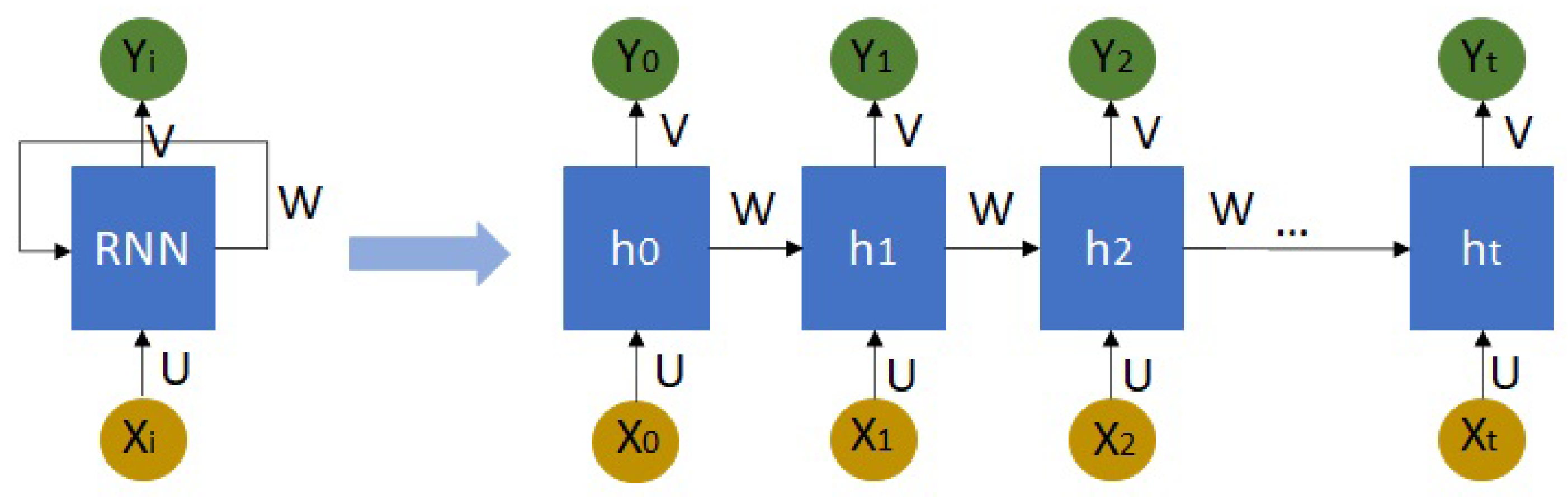
3.1.3. Recurrent Neural Networks

When mentioning RNNs, we refer to neural architectures for processing sequential data and time series usually encountered in tasks, such as bitcoin price prediction [124], speech recognition [125], and machine translation [126]. It is worth noting that implementing RNNs in problems related to natural language processing (NLP) leads to improved results compared to CNNs in most cases [127]. Concerning their functionality and compared to other types of networks (e.g., the multilayer perceptron (MLP) and CNN, which map a given input representation to an output vector), an RNN can estimate an output vector taking into account the entire history of a sequence of previous inputs [128]. To achieve this, the concept of using memory inside the network’s cells is introduced, indicating that the hidden state of a layer passes to the state of the same layer for the next time step (see Figure 1). In each time step, Equations (4) and (5) are applied in the hidden state and the output, respectively, to estimate their current values. Therefore, we calculate:
h t = t a n h ( W h ( t 1 ) + U X t + b ) ,
Y t = σ ( V h t + c ) ,
where b and c are bias vectors; U, V, and W are weight matrices; and σ is an activation function. Thus, the main advantage of RNNs rests on their ability to share the same weights and biases across time.
Regarding the “vanishing gradients” drawback present in RNNs [129], where the information in earlier time points cannot be retrained effectively over the long term, it denotes that the final prediction depends more on the latter points of the data, ignoring the earlier ones. To overcome this drawback, LSTM (i.e., a variation of the traditional RNN cells) introduces a set of forget and memory gates, aiming for the initial inputs to flow until the final stages of the sequence. The authors subsequently proposed a GRU by forming a simpler version of LSTM in [103].

3.1.4. Techniques to Avoid Over-Fitting

We follow the same training and testing procedure for each of the five CNNs and ViT mentioned above to evaluate their performance in human action recognition based on their spatial analysis. A similar methodology to [57] is adopted in the spatial analysis. As training and testing sets, we use the first split provided by the authors of each dataset. Due to the limited training sets in HMDB51 and UCF101, various techniques were proposed to avoid overfitting [58,93,101]. In particular, the three main techniques used for our evaluation protocol are the following:
  • Increased probability rates are applied to the dropout layer [130]. Following the contemporary literature, very high dropout rates ( p 0.8 ) are proven to perform better [37,57,58,66,93,99,101].
  • Image augmentation, such as random cropping, flipping, and RGB jittering, tends to improve performance, especially when more augmentation techniques are applied [57,58,94,101].
  • Finally, transfer learning is usually adopted for increasing the performance when ImageNet is utilized for previously trained networks, both in the case of the two-stream pipeline [57,93,101] and the CNN feature extractor [37,60,62,67,94,105].
The final predictions generated through the sampled frames of each video are fed into the networks, as well as their corresponding scores (i.e., average, maximum, and voting). In addition, the feature vectors extracted by the CNNs and tiny ViT are fed into the RNN architectures to test the performance for the exact frames when the sequential property is exploited.

3.2. Datasets

This subsection describes the datasets used, aiming to evaluate their performance. More specifically, the selected HMDB51 [84], UCF101 [85], and NTU [86,87] are presented, as well as BU101 [131], which is used for increasing the networks’ performance through transfer learning.

3.2.1. HMDB51

The first dataset consists of 51 classes, each providing 101 clips (video sequences), while the total of clips is 6766. Furthermore, the frames’ height has been set to 240 pixels, and the frames-per-second (FPS) ratio has been set to 30 for every clip. These video sequences have been manually extracted and annotated from various sources (e.g., YouTube and movies). Finally, the 51 actions are grouped into five categories: (i) general facial actions, (ii) facial actions with object manipulation, (iii) general body movements, (iv) body movements with object interaction, and (v) body movements with human interaction. Three splits have been generated for the training and testing procedures. Therefore, 70 videos have been chosen for every class and split for the training set, with 30 for the testing set. Choosing the specific clips and not some random splits is vital for our evaluation since these splits are created to ensure that there are no identical or similar video sequences in both sets. We evaluated the networks on the first of the three splits provided by the authors [84]. This consists of 3571 training and 1531 testing videos.

3.2.2. UCF101

The second dataset constitutes an extension of UCF50 [132], providing 101 classes with 13,320 clips. The frame rate has been fixed at 25, and each clip’s frame resolution is 320 × 240. The video sequences have been downloaded from YouTube. Next, they were grouped again into five categories: (i) human–object interaction, (ii) body motion only, (iii) human–human interaction, (iv) playing musical instruments, and (v) sports. Three splits have been generated for the training and testing procedures, where approximately 9500 and 3700 videos are presented. Similar to HMDB51, specific splits are used and not random so that no identical or similar video sequences exist in either training or testing sets. A similar evaluation protocol was followed for this dataset, wherein the networks are evaluated on the first of the three splits provided by the authors [85]. This consists of 9537 training and 3783 testing videos.

3.2.3. NTU

NTU is one of the largest datasets for human action recognition, contrasting with the aforementioned datasets, which are characterized as small-scale and challenging for deep learning techniques. More specifically, it consisted of 60 classes and was later expanded to 120. Its has three main categories: the daily actions, where 82 classes are included; the medical, where 12 classes are encompassed; and the mutual, where 26 types of activities are incorporated. Apart from the RGB data, the 3D skeletons, the masked depth maps, the full depth maps, and the infrared data are also provided. However, in this work, only the RGB data are utilized. More than 114 thousand videos are included, which have been created by 106 individual subjects, corresponding to 8 million frames. From the 120 classes, we focus on the ones within six specific classes: “pick up”, “sit down”, “stand up”, “squat down”, “cross toe touch”, and “falling down”. These have been selected with the intention of evaluating the networks on their performance to recognize cases of falls. The five non-fall classes include actions that look similar to a depiction of a fall. Regarding the split between train and test videos, the authors propose two types of splits. The cross-subject evaluation involves adding videos from 53 specific subjects to the training set, while the remaining videos are used for testing. The second one is the cross-setup evaluation, where subjects with even IDs are utilized for training, and those with odd IDs are used for testing. In this work, cross-subject evaluation has been chosen with the minor modification of adding the IDs “061”, “062”, “063”, “064”, “065”, “066”, “067”, “068”, “069”, “075”, “087”, “088”, “090”, “096”, “099”, “101”, and “102” to the training set, aiming to achieve a balance between the classes among the splits. Specifically, for the classes “pick up”, “sit down”, “stand up”, and “falling down”, the training and testing sets include 672 and 276 videos, respectively, while for the remaining two classes, 624 are used for training and 336 for testing.

3.2.4. BU101

BU101 is chosen to increase the chosen networks’ performance rather than for evaluation purposes. More specifically, it is used for our models’ training, just as with ImageNet. It contains approximately 23,800 images with 101 classes identical to the ones in UCF101. The visual data was automatically downloaded from the web, while the irrelevant data was filtered out. Finally, 2769 images from Standford40 [133] were added to the initial dataset.

3.3. Experimental Details

The current work has been implemented using Python and the PyTorch deep learning library. All the training and evaluation procedures conducted in our experimental study have been performed on a GeForce RTX 3080 10 GB GPU.

3.3.1. Previously Trained on ImageNet and BU101

It is widely known that the utilization of previously trained networks curtails the duration of the training procedure, and higher performance is usually achieved. Hence, transfer learning constitutes a vital process in human action recognition pipelines, mainly when applied in small datasets (e.g., HMDB51 and UCF101). For instance, ImageNet, one of the most extensive static-image datasets containing more than 1.2 million samples for 1000 classes, is a widely adopted dataset for developing previously trained models. However, most target classes of ImageNet, such as “flowers”, “animals”, and “foods,” are irrelevant to the human activity classes, like “push-ups”, “dribbling”, or “pick-up” (see Figure 2). On the contrary, BU101 is a set of data from the web containing static images that depict a human action, as shown in Figure 3, and has been widely used to enhance the performance of activity identification in video sequences [64,131,134,135].
For the aforementioned reasons, BU101 is selected for training our networks before these are transferred and trained on the target datasets. More specifically, for this process, BU101 was split randomly into two sets (70% for training and 30% for testing). Therefore, the networks’ architecture remained the same as the original version, except for the last classification layer, wherein the number of outputs was set to 101 (i.e., the number of classes in BU101). Before the training on BU101, the networks were previously trained on ImageNet. In addition, the Adam optimizer [137] is also utilized with a learning rate of 10 4 and the cross-entropy loss function. Subsequently, similar image augmentation techniques are applied as in the target datasets.
Next, since these networks are intended to be used as previously trained networks on the target datasets, we saved the models’ weights at the epoch with the highest testing accuracy and the smallest difference between training and testing accuracies. In Table 2, these training and testing sets results are denoted for the corresponding epochs, as mentioned earlier.
No image transformation is applied when accuracy is measured apart from the image resizing (step four). Lastly, the weights of the previously trained networks on ImageNet are loaded via the PyTorch (torch and torchvision) library [138], except for EVA-02-Ti, where the model along with its weights is loaded through the Timm library.

3.3.2. Training

For the training part, a similar procedure to Simonyan and Zisserman [57] is adopted to train the spatial stream. In each epoch, each video frame is randomly chosen to be the network’s input. At the same time, image augmentation techniques are applied at each image frame before it is fed into the networks. Moreover, we do not generate a more extensive synthetic dataset, although we transform every frame according to probability before loading it into the network. Four steps are applied, as presented in Table 3. In particular, step one includes four types of transformations (i.e., random crop with output size 100 × 100, center crop with output size 100 × 100, center crop with output size 224 × 224, and no transformation). Step two comprises five types: random horizontal flip, random vertical flip, 30-degree random rotation, 45-degree random affine transformation, and no transformation. Finally, in step three, four types are included: color jitter, Gaussian blur, random solarize, and without transformation. Consequently, one of the transformations is applied to the frame at each step based on the given probability, as shown in Table 3. Finally, in step four, all the frames are resized to 224 × 224, following the networks’ architecture.
Furthermore, we fine-tuned each network by changing the last layer to match the classes in the target datasets, with 51 outputs for HMDB51, 101 for UCF101, and 6 for NTU. We also increased the probability ratio of the dropout layer before the classification one in EfficientNet-b0 and MobileNet-v3 from p = 0.2 to p = 0.5 and p = 0.8 . In addition, a dropout layer was added before the last dense layer in Shuffle-Net-v2, GhostNet, EVA-02-Ti, and ResNet-50, with p = 0.5 and p = 0.8 . The fine-tuned classifiers are represented in Table 4 for each dataset.
During training, the cross-entropy was utilized as the loss function, and the softmax was used to activate the last layer. However, the optimizer, the learning rate, and the batch size vary among networks. The batch size in each training is a function of the power of 2 (e.g., 64, 128, 256), and according to the dynamics of each network, it is adjusted for the optimization of the GPU’s memory.
As far as the optimizer and the learning rate are concerned, Simonyan and Zisserman [57] used stochastic gradient descent (SGD) with an initial learning rate at 10 2 that decayed one order of magnitude after 14 thousand iterations. Following this approach, we first tested all the networks using the SGD optimizer with a learning rate of 10 3 . Then, the optimizer or (and) the learning rate value was changed if the model was underfitted or overfitted too fast. Table 5 presents this parameterization, which permitted similar and smooth training curves as shown in Figure 4 and Figure 5, where the training and testing losses are represented across epochs for each network and dataset.

3.3.3. Testing

For the testing procedure, we sample 15 frames of each video with an equal temporal difference between them, as depicted in Figure 6 with the blue and orange blocks. A similar method was proposed in [57]; however, they used 25 frames for each video. Our approach is based on the work of Lan et al. [61], wherein, during evaluation, they utilized 3, 9, 15, 21, and 25 frames on the same datasets. Notably, in various works [57,58,93], the initially chosen frames extract more images for evaluation by applying cropping or flipping techniques. Nevertheless, in the proposed work, the final prediction only comes from the initial frames. Subsequently, inspired by the TSN method [101], each video is split into three equal segments, and one frame is selected randomly for evaluation (see the green part in Figure 6). The final class for a whole video is obtained in three different ways according to the outputs of the networks:
  • by averaging the scores of all the sampled frames: max ( i = 0 n s c o r e s i n ) f i n a l _ c l a s s ;
  • by taking as a final prediction the class with the highest score:
    max ( max ( s c o r e s 0 ) , , max ( s c o r e s n ) ) f i n a l _ c l a s s ;
  • by applying the voting method and taking as the final prediction the class with the most votes: m o s t _ f r e q u e n t ( c l a s s 0 , , c l a s s n ) f i n a l _ c l a s s .

3.4. Training and Testing of the RNNs

The same 15 sampled frames presenting equal temporal intervals are exploited to evaluate three types of RNNs (i.e., the simple RNN cell, the LSTM, and the GRU). The above-mentioned frames are fed into the CNNs and ViT, which are utilized as feature extractors [37,60,62,67,94,105], and the extracted feature vectors are passed to the recurrent architectures. We utilize the networks that achieve the highest accuracies on the spatial analysis. These are employed after training on the target datasets and after being previously trained on ImageNet+BU101. EfficientNet-b0 is utilized with p = 0.5 on the dropout layer for both HMDB51 and UCF101; ResNet-50 with p = 0.8 and p = 0.5 , for HMDB51 and UCF101, respectively; and EVA-02-Ti with p = 0.5 , for both datasets. For the NTU dataset, the networks trained without a dropout layer due to its large size. Table 4 shows how the last layers of each network extract the feature vector. Each frame of EfficientNet-b0 is represented by a feature vector of 1280 bins. The output of EVA-02-Ti is 192, and that of ResNet-50 is 2048.
All RNNs are trained using the same parameters. We employ one hidden layer with 512 units, similar to [60,94]. The batch size is 256, adopting the SGD optimizer with a learning rate at 10 3 . For weight optimization, the common cross-entropy loss function is employed. The output of each RNN is fed into an FC classification layer, with 51 output neurons for HMDB51 and 101 for UCF101. During training, the RNNs’ input is the feature vectors from the 15 sampled frames with equal space between them. Two types of training were applied. In the first, the final prediction comes from all the hidden states (i.e., fifteen frames); in the second one, prediction is generated from the last hidden state. That means that in the first type, the input of the classification layer is 512 × 15 = 7680 , and when the final prediction comes from the last hidden state, the input of the classification layer is 512 × 1 = 512 . During testing, the RNNs’ input is the 15 feature vectors from the sampled frames. These have been used for average, max scores, and voting predictions.

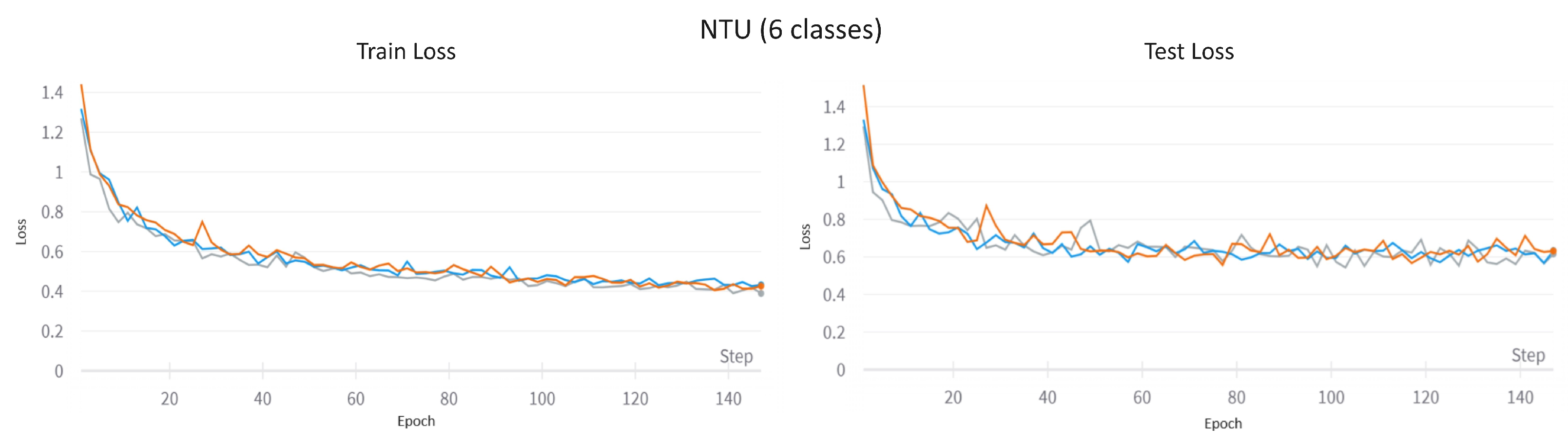
4. Experimental Results

Table 6, Table 7 and Table 8 present the achieved accuracies following the aforementioned testing protocol for each network on HMDB51, UCF101, and NTU, respectively. Additionally, the tables include information on the training process types, specifically the dropout layer rates and the used datasets for transfer learning.
Regarding HMDB51, from Table 6, it is observed that Shufflenet-v2 achieves the lowest performance at 45%, followed by GhostNet at 50.21%, EVA-02-Ti at 50.34%, and MobileNet-v3 at 50.57%. ResNet-50 and Efficient-b0 exhibit the highest accuracies at 55.03% and 55.50%, respectively. In all cases, the average testing approaches outperform the maximum and voting methods, while the average scores based on 3 frames have similar metrics to those obtained by 15 frames. Regarding the training process, the greater scores are secured when the models have previously been trained on both ImageNet and BU101, and a dropout layer of high rate, p = 0.8 , has been applied before the last FC. EVA-02-Ti is the only exception, where the dropout rate at p = 0.5 and ImageNet for transfer learning outperforms the other approaches.
Regarding the results for UCF101 (see Table 7), Shufflenet-v2 has the lowest performance at 75.17%, followed by MobileNet at 82.97%, and GhostNet at 83.16%. The accuracies of EVA-02-Ti and Efficient-b0 are close at 86.04% and 86.10%, respectively, while ResNet-50 outperforms all the networks at 87.45%. Once again, the average results outperform the other two methods, and utilizing 3 frames yields performances very close to those with 15 frames. Regarding the training procedures, the optimal accuracies are secured when the models are previously trained on ImageNet and BU101. At the same time, a dropout rate set at p = 0.5 is applied on EVA-02-Ti and ResNet-50. In the remaining four networks, the dropout rate set at p = 0.8 generates better metrics.
As represented in Table 8, the three networks that achieved the highest performances on the previous datasets are evaluated on the NTU dataset, specifically the mobile-CNN EfficientNet-b0, the tiny ViT EVA-02-Ti, and the higher-computational-cost CNN ResNet-50. With accuracies of 86.27% and 84.84% on 3 and 15 frames (average score), respectively, the ViT outperforms the other two networks. EfficientNet-b0 achieves 85.59% and 85.20%, while ResNet-50 achieves 85.46%, and 84.72%, on 3 and 15 frames, respectively. Consistent with previous observations, on HMDB51 and UCF101, the averaging scores outperform both the maximum and voting approaches.
Table 9 presents the accuracy measurements from the temporal analysis, implemented by the RNNs, for HMDB51, UCF101, and NTU. For each RNN type (i.e., RNN, LSTM, and GRU), two measurements are provided according to the set of the outputs (i.e., all the outputs or the final output, are used on the classification layer). Furthermore, three dyads are presented for each RNN based on the model (i.e., EfficientNet-b0, EVA-02-Ti, and ResNet-50) used as the feature extractor method. Finally, for the corresponding networks, the highest accuracies according to the average scores of the 15 sampled frames are provided for comparison against the RNNs, which were trained and tested with the same 15 frames. Regarding the results on both HMDB51 and UCF101, it appears that the contribution of the RNNs does not significantly improve the results, as the accuracies either remain close to those of the spatial analysis or even drop to lower levels. On the other hand, the performance on the NTU dataset reaches very high levels, exceeding 94.00% accuracy in all the cases, while in the spatial analysis, it was close to 85.00%. Notably, the RNN that utilizes all 15 outputs at the classification layer achieves the highest metrics across all three configurations of networks as feature extractors. Specifically, for Efficient-b0, the accuracy increases from 85.59%. Additionally, in the case of EVA-02-Ti, it rises from 86.27% to 97.63%, and for ResNet-50, it improves from 85.46% to 97.07%.

5. Fall Recognition Analysis on the NTU Dataset

As fall recognition is one of the main objectives in action recognition within the computer vision field [10,139,140,141,142], Table 10 presents the results of all approaches in their capacity to distinguish falls from the other five similar actions in the NTU dataset. The fall recognition problem is approached as a binary classification task, where either a fall or a daily action is depicted in the video. "Fall" is considered the positive class, while the remaining five are the negative class. It is important to note that no additional training was implemented, but all the classes apart from "fall" are grouped as one in the testing process. Furthermore, the metrics used for the evaluation of the networks and approaches in fall recognition are sensitivity, specificity, and precision, as represented in Equations (6), (7), and (8), respectively. Sensitivity assesses the model’s ability to accurately detect falls, while specificity measures its performance in handling non-fall cases. A high sensitivity score indicates that the system can effectively detect most accidents, while specificity ensures low false positive detections. However, in this specific test set, an imbalance is evident, as it includes 1500 non-fall videos and just 276 examples of falls. The precision metric is also illustrated, indicating the performance of the networks in detecting true positive instances.
Sensitivity = Recall = True Positives True Positives + False Negatives
Specificity = True Negatives True Negatives + False Positives
Precision = True Positives True Positives + False Positive
As expected, given the previously high performance of temporal analysis on the six classes of NTU, all the metrics referring to the RNNs are above 95.00%. Furthermore, in terms of spatial analysis, it is also observed that the models can distinguish accidents from other daily actions. The highest scores are secured by utilizing all 15 frames, from ResNet-50 at 92.52%, followed by EVA-02-Ti at 90.62%, with EfficientNet-b0 lagging behind at 89.18%. Regarding sensitivity, the mobile-CNN and ResNet-50, using 15 frames, achieve 95.65% and 94.20%, respectively, while the tiny ViT, which utilizes 3 frames, performs at 94.56%. The specificity is over 97.50% in all cases, but the dominance of the negative class influences these high rates.
Moreover, regarding the less computational approach, where only three frames are utilized, EfficientNet-b0 outperforms the other networks on sensitivity, while EVA-02-Ti achieves higher precision and specificity. Therefore, the lightweight networks can be compared to ResNet-50 on the fall recognition task. Finally, we would like to highlight that these results provide a preliminary analysis of the specific six classes of the NTU. Further experiments on datasets specifically designed for fall detection are imperative for more accurate conclusions.

6. Discussion

As shown from the results in Table 6 and Table 7, the average score achieves higher accuracy than the max score and voting in every network and training procedure. Furthermore, networks previously trained on ImageNet and BU101 perform with higher accuracy than the ones previously trained only on ImageNet. The only exception is MobileNet-v3 and EVA-02-Ti, previously trained on ImageNet, which achieve better accuracy according to the average score of the 15 sampled frames in HMDB51. Additionally, the dropout probability ratio of 80% achieves higher accuracy than the 50% one in all cases, apart from the ShuffleNet-v2 trained on HMDB51, the ResNet-50 on UCF101, and the EVA-02-Ti on both UCF101 and HMDB51.
Regarding spatial analysis, using a total of 15 frames generally performs better than using only 3 frames. However, the difference between the two highest accuracies of 15 and 3 frames is no more than 1.49% (see EfficientNet-b0 on HMDB51), reflecting that if the computational power is limited, the processing and analysis of just 3 frames can be applied to reduce the latency, while achieving similar performance as with 15 frames, as initially supported and proposed by [101,143]. Among mobile-CNNs, ShuffleNet-v2 is the weakest model, based on the results of the first two datasets, whereas EfficientNet-b0 is the most powerful, achieving similar, or even superior, performance to ResNet-50. Additionally, the ViT EVA-02-Ti outperforms the mobile-CNNs, apart from EfficientNet-b0, which in HMDB51 lags by a margin of five percentage points, while in UCF101, they have almost identical performance.
Moreover, in all the cases, it is observed that the models do not efficiently distinguish between classes in HMDB51 (see Table 6) compared to UCF101, where better performance is achieved (see Table 7). Both datasets can be characterized as challenging for deep learning approaches, given their limited size, as HMDB51 contains 70 videos per class for training, while UCF101 has an average of 95. As a result, deep learning models quickly transition from underfitting to overfitting without achieving a balanced, unbiased network. Hence, a lot of techniques to avoid over-fitting are applied (viz., image augmentation, transfer learning, and dropout layers with high rates). However, HMDB51 is a more challenging dataset than UCF101, as it contains fewer training videos, leading to this performance gap, while differences between the results on these two datasets have also been identified by multiple approaches (e.g., in [21,57,144]). Finally, regarding the performance of the models on smaller datasets, the ResNet-50 models, with higher computational costs compared to mobile-CNNs, and especially the ViT, require a larger amount of training as they are susceptible to over-fitting on limited datasets.
On the contrary, the NTU is one of the largest datasets on action recognition, and it was created in a controlled environment by subjects who were performing the actions. Specifically, in the applied six classes, with the modification utilized in the training IDs, each class contains more than 600 training videos. In this section, EVA-02-Ti outperforms EfficientNet-b0 and ResNet-50 in both frame approaches by achieving 86.27% and 84.84% for 3 and 15 frames, respectively. However, all the networks attain similar accuracies in both sets of frames, with their differences being smaller than 0.64%.
In terms of the temporal analysis performance with RNNs on HMDB51 and UCF101, no improvement is observed, as the accuracies do not surpass those obtained through spatial analysis. The only exception is in HMDB51, where the RNN, utilizing all the outputs and EVA-02-Ti employed as feature extractor, has an accuracy of 53.03%, while the spatial analysis is 50.07%. On the contrary, the results exhibit a marked difference when applying RNNs to the NTU dataset. Notably, while the metrics from spatial analysis using CNNs and ViT mirror those of UCF101, all types of RNNs achieve a performance exceeding 94%, with RNNs utilizing all 15 outputs to the last FC layer outperforming LSTM and GRU. Specifically, features from EVA-02-Ti result in an accuracy of 97.63%; from ResNet-50, it is 97.07%; and from EfficientNet-b0, it is 96.39%. Based on the aforementioned findings, it is evident that the tiny ViT produces superior feature vectors, while the most lightweight model, EfficientNet-b0, generates vectors that achieve similar performance through RNNs, making it a viable choice, especially when computational resources are limited.
The sharp difference between the performances achieved by RNNs on the NTU, compared to HMDB51 and UCF101, is likely a result of the distinct nature of the NTU dataset, influencing the networks to generate more enlightening vectors [26]. The NTU dataset includes significantly more training points than HMDB51 and UCF101, and it has been created under controlled environments and with specific subjects who carry out the actions. In contrast, HMDB51 and UCF101 contain entirely different videos, such as movie scenes and YouTube videos. Additionally, the fact that we applied fewer total classes (6 out of 120) for the NTU dataset, compared to HMDB51 and UCF101, with 51 and 101 classes, respectively, could potentially impact the performance metrics. However, it is worth noting that such an impact is not observed in the spatial analysis between UCF101 and NTU. Aiming to explain why RNNs outperform LSTM and GRU, we analyzed video clips where key action segments are mostly positioned in the middle or at the end. This could turn the “vanishing gradients” [129] drawback of RNNs into an advantage, as the earlier information strives to endure over the long term, and the final prediction depends more on the latter points of the data. However, this is only a hypothesis and not a conclusion.
Additionally, the RNNs in HMDB51 and UCF101 can achieve higher performance if different training or testing strategies are applied. Such strategies could include end-to-end training [37], the training of only specific layers [62], the use of more (or fewer) frames in the training/test part [37,94,105], and different approaches for the final prediction like max pooling, summing, linearly weighting [60], and average score [37]. Furthermore, the additional use of optical flow on RNNs can enhance the final classification performance [37,60].

7. Conclusions

This article presented a quantitative and qualitative evaluation protocol for four mobile-CNNs and a tiny ViT for human action recognition. Aiming to facilitate future robotics-oriented implementations, we conducted experiments based on the networks’ spatial and temporal analysis. This way, boundaries and limitations concerning the outcome and computational complexity have been studied. As our results show, EffiecientNet-b0 and ResNet-50 perform similarly on the small-scale HMDB51 and UCF101, while MobileNet-v3 and GhostNet outperform ShuffleNet-v2; however, they cannot compete with EfficientNet-b0. In addition, EVA-02-Ti performs similarly to EfficientNet-b0 on UCF101, while HMDB51 is close to GhostNet’s accuracy. Another finding of ours, which agrees with the literature, regards the dropout layer probability. In particular, higher outcomes are attained during training using a higher probability before the last classification layer, apart from EVA-02-Ti, which performs better with the lower dropout rate despite the limited size of the datasets. Moreover, networks previously trained on ImageNet and BU101 can reach higher accuracy scores than those trained only on ImageNet, as was expected due to their relevance to the videos of the target datasets. Regarding the temporal analysis through RNNs, which utilized the trained networks as feature extractors of frames, their application did not lead to improved results in the two challenging datasets. In the six classes of NTU, the three evaluated networks—EfficientNet-bo, EVA-02-Ti, and ResNet-50—attain comparable results in spatial analysis, while the ViT outperforms the CNNs. In the temporal approach, unlike in the aforementioned datasets, all the RNNs enhance the performance, regardless of which network is used as an extractor. Consequently, for a lightweight system, the mobile-CNN EfficientNet-b0 and the tiny ViT EVA-02-Ti can be applied, as they have achieved similar or even, in some cases, superior results compared to the higher-computational-cost CNN, ResNet-50. In particular, EfficientNet-b0, being the lightest network in terms of total FLOPs and parameters, could be the optimal choice for action recognition, especially if the minor superiority of ViT on large datasets does not outweigh its higher complexity. Moreover, concerning spatial analysis, performance comparable to that with 15 frames can be achieved when the classification is based on only 3 frames, thereby reducing latency. Furthermore, RNNs, as observed in temporal analysis, appear more effective when applied to large-scale datasets. Our plans include evaluation of the attention-based approaches for temporal analysis instead of the conventional RNNs.

Author Contributions

Conceptualization, S.N.M., K.A.T. and I.K.; methodology, S.N.M.; software, S.N.M.; validation, S.N.M., K.A.T., I.K. and A.G.; formal analysis, K.A.T. and I.K.; investigation, K.A.T. and I.K.; resources, S.N.M.; data curation, S.N.M. and K.A.T.; writing—original draft preparation, S.N.M.; writing—review and editing, K.A.T., I.K. and A.G.; visualization, S.N.M.; supervision, A.G.; project administration, K.A.T. and A.G.; funding acquisition, A.G. All authors have read and agreed to the published version of the manuscript.

Funding

This research was funded by “Wearable systems for the safety and wellbeing applied in security guards—SafeIT” which has been financially supported by the European Union and Greek national funds through the Operational Program Competitiveness, Entrepreneurship and Innovation, under the call RESEARCH–CREATE–INNOVATE grant number [T2EDK-01862].

Data Availability Statement

The original contributions presented in the study are included in the article; further inquiries can be directed to the corresponding author.

Acknowledgments

Portions of the research in this paper used the NTU RGB+D 120 Action Recognition Dataset made available by the ROSE Lab at the Nanyang Technological University, Singapore.

Conflicts of Interest

The authors declare no conflict of interest. The funders had no role in the design of the study; in the collection, analyses, or interpretation of data; in the writing of the manuscript; or in the decision to publish the results.

References

  1. Zhang, H.B.; Zhang, Y.X.; Zhong, B.; Lei, Q.; Yang, L.; Du, J.X.; Chen, D.S. A comprehensive survey of vision-based human action recognition methods. Sensors 2019, 19, 1005. [Google Scholar] [CrossRef] [PubMed]
  2. Arseneau, S.; Cooperstock, J.R. Real-time image segmentation for action recognition. In Proceedings of the 1999 IEEE Pacific Rim Conference on Communications, Computers and Signal Processing (PACRIM 1999), Conference Proceedings (Cat. No. 99CH36368), Victoria, BC, Canada, 22–24 August 1999; IEEE: Piscataway, NJ, USA, 1999; pp. 86–89. [Google Scholar]
  3. Masoud, O.; Papanikolopoulos, N. A method for human action recognition. Image Vis. Comput. 2003, 21, 729–743. [Google Scholar] [CrossRef]
  4. Charalampous, K.; Gasteratos, A. A tensor-based deep learning framework. Image Vis. Comput. 2014, 32, 916–929. [Google Scholar] [CrossRef]
  5. Gammulle, H.; Ahmedt-Aristizabal, D.; Denman, S.; Tychsen-Smith, L.; Petersson, L.; Fookes, C. Continuous Human Action Recognition for Human-Machine Interaction: A Review. arXiv 2022, arXiv:2202.13096. [Google Scholar] [CrossRef]
  6. An, S.; Zhou, F.; Yang, M.; Zhu, H.; Fu, C.; Tsintotas, K.A. Real-time monocular human depth estimation and segmentation on embedded systems. In Proceedings of the 2021 IEEE/RSJ International Conference on Intelligent Robots and Systems (IROS), Prague, Czech Republic, 27 September–1 October 2021; IEEE: Piscataway, NJ, USA, 2021; pp. 55–62. [Google Scholar]
  7. Yin, J.; Han, J.; Wang, C.; Zhang, B.; Zeng, X. A skeleton-based action recognition system for medical condition detection. In Proceedings of the 2019 IEEE Biomedical Circuits and Systems Conference (BioCAS), Nara, Japan, 17–19 October 2019; IEEE: Piscataway, NJ, USA, 2019; pp. 1–4. [Google Scholar]
  8. Cóias, A.R.; Lee, M.H.; Bernardino, A. A low-cost virtual coach for 2D video-based compensation assessment of upper extremity rehabilitation exercises. J. Neuroeng. Rehabil. 2022, 19, 1–16. [Google Scholar] [CrossRef]
  9. Moutsis, S.N.; Tsintotas, K.A.; Gasteratos, A. PIPTO: Precise Inertial-Based Pipeline for Threshold-Based Fall Detection Using Three-Axis Accelerometers. Sensors 2023, 23, 7951. [Google Scholar] [CrossRef]
  10. Moutsis, S.N.; Tsintotas, K.A.; Kansizoglou, I.; An, S.; Aloimonos, Y.; Gasteratos, A. Fall detection paradigm for embedded devices based on YOLOv8. In Proceedings of the IEEE International Conference on Imaging Systems and Techniques, Copenhagen, Denmark, 1 May–19 October 2023; pp. 1–6. [Google Scholar]
  11. Hoang, V.D.; Hoang, D.H.; Hieu, C.L. Action recognition based on sequential 2D-CNN for surveillance systems. In Proceedings of the IECON 2018—44th Annual Conference of the IEEE Industrial Electronics Society, Washington, DC, USA, 21–23 October 2018; IEEE: Piscataway, NJ, USA, 2018; pp. 3225–3230. [Google Scholar]
  12. Tsintotas, K.A.; Bampis, L.; Taitzoglou, A.; Kansizoglou, I.; Kaparos, P.; Bliamis, C.; Yakinthos, K.; Gasteratos, A. The MPU RX-4 project: Design, electronics, and software development of a geofence protection system for a fixed-wing vtol uav. IEEE Trans. Instrum. Meas. 2022, 72, 7000113. [Google Scholar] [CrossRef]
  13. Wei, D.; An, S.; Zhang, X.; Tian, J.; Tsintotas, K.A.; Gasteratos, A.; Zhu, H. Dual Regression for Efficient Hand Pose Estimation. In Proceedings of the 2022 International Conference on Robotics and Automation (ICRA), Philadelphia, PA, USA, 23–27 May 2022; IEEE: Piscataway, NJ, USA, 2022; pp. 6423–6429. [Google Scholar]
  14. Carvalho, M.; Avelino, J.; Bernardino, A.; Ventura, R.; Moreno, P. Human-Robot greeting: Tracking human greeting mental states and acting accordingly. In Proceedings of the 2021 IEEE/RSJ International Conference on Intelligent Robots and Systems (IROS), Prague, Czech Republic, 27 September–1 October 2021; IEEE: Piscataway, NJ, USA, 2021; pp. 1935–1941. [Google Scholar]
  15. An, S.; Zhang, X.; Wei, D.; Zhu, H.; Yang, J.; Tsintotas, K.A. FastHand: Fast monocular hand pose estimation on embedded systems. J. Syst. Archit. 2022, 122, 102361. [Google Scholar] [CrossRef]
  16. Charalampous, K.; Kostavelis, I.; Gasteratos, A. Robot navigation in large-scale social maps: An action recognition approach. Expert Syst. Appl. 2016, 66, 261–273. [Google Scholar] [CrossRef]
  17. Tsintotas, K.A.; Bampis, L.; Gasteratos, A. Online Appearance-Based Place Recognition and Mapping: Their Role in Autonomous Navigation; Springer Nature: Berlin/Heidelberg, Germany, 2022; Volume 133. [Google Scholar]
  18. Herath, S.; Harandi, M.; Porikli, F. Going deeper into action recognition: A survey. Image Vis. Comput. 2017, 60, 4–21. [Google Scholar] [CrossRef]
  19. Poppe, R. A survey on vision-based human action recognition. Image Vis. Comput. 2010, 28, 976–990. [Google Scholar] [CrossRef]
  20. Bobick, A.F.; Davis, J.W. The recognition of human movement using temporal templates. IEEE Trans. Pattern Anal. Mach. Intell. 2001, 23, 257–267. [Google Scholar] [CrossRef]
  21. Wang, H.; Schmid, C. Action recognition with improved trajectories. In Proceedings of the IEEE International Conference on Computer Vision, Sydney, Australia, 1–8 December 2013; pp. 3551–3558. [Google Scholar]
  22. Tsintotas, K.A.; Giannis, P.; Bampis, L.; Gasteratos, A. Appearance-based loop closure detection with scale-restrictive visual features. In Proceedings of the International Conference on Computer Vision Systems, Thessaloniki, Greece, 23–25 September 2019; Springer: Cham, Switzerland, 2019; pp. 75–87. [Google Scholar]
  23. Li, W.; Zhang, Z.; Liu, Z. Action recognition based on a bag of 3D points. In Proceedings of the 2010 IEEE Computer Society Conference on Computer Vision and Pattern Recognition-Workshops, San Francisco, CA, USA, 13–18 June 2010; IEEE: Piscataway, NJ, USA, 2010; pp. 9–14. [Google Scholar]
  24. Zhang, S.; Wei, Z.; Nie, J.; Huang, L.; Wang, S.; Li, Z. A review on human activity recognition using vision-based method. J. Healthc. Eng. 2017, 2017, 3090343. [Google Scholar] [CrossRef] [PubMed]
  25. Kansizoglou, I.; Bampis, L.; Gasteratos, A. Do neural network weights account for classes centers? IEEE Trans. Neural Netw. Learn. Syst. 2022, 34, 8815–8824. [Google Scholar] [CrossRef] [PubMed]
  26. Kansizoglou, I.; Bampis, L.; Gasteratos, A. Deep feature space: A geometrical perspective. IEEE Trans. Pattern Anal. Mach. Intell. 2021, 44, 6823–6838. [Google Scholar] [CrossRef] [PubMed]
  27. Simonyan, K.; Zisserman, A. Very deep convolutional networks for large-scale image recognition. arXiv 2014, arXiv:1409.1556. [Google Scholar]
  28. Redmon, J.; Divvala, S.; Girshick, R.; Farhadi, A. You only look once: Unified, real-time object detection. In Proceedings of the IEEE Conference on Computer Vision and Pattern Recognition, Las Vegas, NV, USA, 26 June–1 July 2016; pp. 779–788. [Google Scholar]
  29. Tsintotas, K.A.; Bampis, L.; Taitzoglou, A.; Kansizoglou, I.; Gasteratos, A. Safe UAV landing: A low-complexity pipeline for surface conditions recognition. In Proceedings of the IEEE International Conference on Imaging Systems and Techniques (IST), Virtual, 24–26 August 2021; pp. 1–6. [Google Scholar]
  30. An, S.; Zhu, H.; Wei, D.; Tsintotas, K.A.; Gasteratos, A. Fast and incremental loop closure detection with deep features and proximity graphs. J. Field Robot. 2022, 39, 473–493. [Google Scholar] [CrossRef]
  31. Tsintotas, K.A.; Sevetlidis, V.; Papapetros, I.T.; Balaska, V.; Psomoulis, A.; Gasteratos, A. BK tree indexing for active vision-based loop-closure detection in autonomous navigation. In Proceedings of the 2022 30th Mediterranean Conference on Control and Automation (MED), Athens, Greece, 28 June–1 July 2022; pp. 532–537. [Google Scholar]
  32. Tsintotas, K.A.; Bampis, L.; Gasteratos, A. Probabilistic appearance-based place recognition through bag of tracked words. IEEE Robot. Autom. Lett. 2019, 4, 1737–1744. [Google Scholar] [CrossRef]
  33. Tsintotas, K.A.; Bampis, L.; Gasteratos, A. Tracking-DOSeqSLAM: A dynamic sequence-based visual place recognition paradigm. IET Comput. Vis. 2021, 15, 258–273. [Google Scholar] [CrossRef]
  34. Tsintotas, K.A.; Bampis, L.; Gasteratos, A. Visual Place Recognition for Simultaneous Localization and Mapping. In Autonomous Vehicles Volume 2: Smart Vehicles; Scrivener Publishing LLC: Beverly, MA, USA, 2022; pp. 47–79. [Google Scholar]
  35. Tsintotas, K.A.; Bampis, L.; Gasteratos, A. Modest-vocabulary loop-closure detection with incremental bag of tracked words. Robot. Auton. Syst. 2021, 141, 103782. [Google Scholar] [CrossRef]
  36. Tsintotas, K.A.; Bampis, L.; Gasteratos, A. The Revisiting Problem in Simultaneous Localization and Mapping: A Survey on Visual Loop Closure Detection. IEEE Trans. Intell. Transp. Syst. 2022, 23, 19929–19953. [Google Scholar] [CrossRef]
  37. Donahue, J.; Anne Hendricks, L.; Guadarrama, S.; Rohrbach, M.; Venugopalan, S.; Saenko, K.; Darrell, T. Long-term recurrent convolutional networks for visual recognition and description. In Proceedings of the IEEE Conference on Computer Vision and Pattern Recognition, Boston, MA, USA, 7–12 June 2015; pp. 2625–2634. [Google Scholar]
  38. Oikonomou, K.M.; Kansizoglou, I.; Gasteratos, A. A Framework for Active Vision-Based Robot Planning using Spiking Neural Networks. In Proceedings of the 2022 30th Mediterranean Conference on Control and Automation (MED), Vouliagmeni, Greece, 28 June–1 July 2022; IEEE: Piscataway, NJ, USA, 2022; pp. 867–871. [Google Scholar]
  39. LeCun, Y.; Bottou, L.; Bengio, Y.; Haffner, P. Gradient-based learning applied to document recognition. Proc. IEEE 1998, 86, 2278–2324. [Google Scholar] [CrossRef]
  40. Krizhevsky, A.; Sutskever, I.; Hinton, G.E. Imagenet classification with deep convolutional neural networks. Commun. ACM 2017, 60, 84–90. [Google Scholar] [CrossRef]
  41. Szegedy, C.; Liu, W.; Jia, Y.; Sermanet, P.; Reed, S.; Anguelov, D.; Erhan, D.; Vanhoucke, V.; Rabinovich, A. Going deeper with convolutions. In Proceedings of the IEEE Conference on Computer Vision and Pattern Recognition, Boston, MA, USA, 7–12 June 2015; pp. 1–9. [Google Scholar]
  42. Ioffe, S.; Szegedy, C. Batch normalization: Accelerating deep network training by reducing internal covariate shift. In Proceedings of the International Conference on Machine Learning, PMLR, Lille, France, 7–9 July 2015; pp. 448–456. [Google Scholar]
  43. He, K.; Zhang, X.; Ren, S.; Sun, J. Deep residual learning for image recognition. In Proceedings of the IEEE Conference on Computer Vision and Pattern Recognition, Las Vegas, NV, USA, 26 June–1 July 2016; pp. 770–778. [Google Scholar]
  44. Deng, J.; Dong, W.; Socher, R.; Li, L.J.; Li, K.; Fei-Fei, L. Imagenet: A large-scale hierarchical image database. In Proceedings of the 2009 IEEE Conference on Computer Vision and Pattern Recognition, Miami, FL, USA, 20–25 June 2009; IEEE: Piscataway, NJ, USA, 2009; pp. 248–255. [Google Scholar]
  45. Russakovsky, O.; Deng, J.; Su, H.; Krause, J.; Satheesh, S.; Ma, S.; Huang, Z.; Karpathy, A.; Khosla, A.; Bernstein, M.; et al. Imagenet large scale visual recognition challenge. Int. J. Comput. Vis. 2015, 115, 211–252. [Google Scholar] [CrossRef]
  46. Howard, A.G.; Zhu, M.; Chen, B.; Kalenichenko, D.; Wang, W.; Weyand, T.; Andreetto, M.; Adam, H. Mobilenets: Efficient convolutional neural networks for mobile vision applications. arXiv 2017, arXiv:1704.04861. [Google Scholar]
  47. Sandler, M.; Howard, A.; Zhu, M.; Zhmoginov, A.; Chen, L.C. Mobilenetv2: Inverted residuals and linear bottlenecks. In Proceedings of the IEEE Conference on Computer Vision and Pattern Recognition, Salt Lake City, UT, USA, 18–23 June 2018; pp. 4510–4520. [Google Scholar]
  48. Zhang, X.; Zhou, X.; Lin, M.; Sun, J. Shufflenet: An extremely efficient convolutional neural network for mobile devices. In Proceedings of the IEEE Conference on Computer Vision and Pattern Recognition, Salt Lake City, UT, USA, 18–23 June 2018; pp. 6848–6856. [Google Scholar]
  49. Ma, N.; Zhang, X.; Zheng, H.T.; Sun, J. Shufflenet v2: Practical guidelines for efficient cnn architecture design. In Proceedings of the European Conference on Computer Vision (ECCV), Munich, Germany, 8–14 September 2018; pp. 116–131. [Google Scholar]
  50. Zoph, B.; Vasudevan, V.; Shlens, J.; Le, Q.V. Learning transferable architectures for scalable image recognition. In Proceedings of the IEEE Conference on Computer Vision and Pattern Recognition, Salt Lake City, UT, USA, 18–23 June 2018; pp. 8697–8710. [Google Scholar]
  51. Wu, B.; Dai, X.; Zhang, P.; Wang, Y.; Sun, F.; Wu, Y.; Tian, Y.; Vajda, P.; Jia, Y.; Keutzer, K. Fbnet: Hardware-aware efficient convnet design via differentiable neural architecture search. In Proceedings of the IEEE/CVF Conference on Computer Vision and Pattern Recognition, Long Beach, CA, USA, 15–20 June 2019; pp. 10734–10742. [Google Scholar]
  52. Tan, M.; Le, Q. Efficientnet: Rethinking model scaling for convolutional neural networks. In Proceedings of the International Conference on Machine Learning, PMLR, Long Beach, CA, USA, 9–15 June 2019; pp. 6105–6114. [Google Scholar]
  53. Howard, A.; Sandler, M.; Chu, G.; Chen, L.C.; Chen, B.; Tan, M.; Wang, W.; Zhu, Y.; Pang, R.; Vasudevan, V.; et al. Searching for mobilenetv3. In Proceedings of the IEEE/CVF International Conference on Computer Vision, Seoul, Republic of Korea, 27 October–2 November 2019; pp. 1314–1324. [Google Scholar]
  54. Han, K.; Wang, Y.; Tian, Q.; Guo, J.; Xu, C.; Xu, C. Ghostnet: More features from cheap operations. In Proceedings of the IEEE/CVF Conference on Computer Vision and Pattern Recognition, Seattle, WA, USA, 13–19 June 2020; pp. 1580–1589. [Google Scholar]
  55. Huo, Y.; Xu, X.; Lu, Y.; Niu, Y.; Lu, Z.; Wen, J.R. Mobile video action recognition. arXiv 2019, arXiv:1908.10155. [Google Scholar]
  56. Chatfield, K.; Simonyan, K.; Vedaldi, A.; Zisserman, A. Return of the devil in the details: Delving deep into convolutional nets. arXiv 2014, arXiv:1405.3531. [Google Scholar]
  57. Simonyan, K.; Zisserman, A. Two-stream convolutional networks for action recognition in videos. Adv. Neural Inf. Process. Syst. 2014, 27, 568–576. [Google Scholar]
  58. Wang, L.; Xiong, Y.; Wang, Z.; Qiao, Y. Towards good practices for very deep two-stream convnets. arXiv 2015, arXiv:1507.02159. [Google Scholar]
  59. Zeiler, M.D.; Fergus, R. Visualizing and understanding convolutional networks. In Proceedings of the European Conference on Computer Vision, Zurich, Switzerland, 6–12 September 2014; Springer: Cham, Switzerland, 2014; pp. 818–833. [Google Scholar]
  60. Yue-Hei Ng, J.; Hausknecht, M.; Vijayanarasimhan, S.; Vinyals, O.; Monga, R.; Toderici, G. Beyond short snippets: Deep networks for video classification. In Proceedings of the IEEE Conference on Computer Vision and Pattern Recognition, Boston, MA, USA, 7–12 June 2015; pp. 4694–4702. [Google Scholar]
  61. Lan, Z.; Zhu, Y.; Hauptmann, A.G.; Newsam, S. Deep local video feature for action recognition. In Proceedings of the IEEE Conference on Computer Vision and Pattern Recognition Workshops, Honolulu, HI, USA, 21–26 July 2017; pp. 1–7. [Google Scholar]
  62. Chenarlogh, V.A.; Jond, H.B.; Platoš, J. A Robust Deep Model for Human Action Recognition in Restricted Video Sequences. In Proceedings of the 2020 43rd International Conference on Telecommunications and Signal Processing (TSP), Milan, Italy, 7–9 July 2020; IEEE: Piscataway, NJ, USA, 2020; pp. 541–544. [Google Scholar]
  63. Zhang, Y.; Guo, Q.; Du, Z.; Wu, A. Human Action Recognition for Dynamic Scenes of Emergency Rescue Based on Spatial-Temporal Fusion Network. Electronics 2023, 12, 538. [Google Scholar] [CrossRef]
  64. Li, J.; Wong, Y.; Zhao, Q.; Kankanhalli, M.S. Attention transfer from web images for video recognition. In Proceedings of the 25th ACM International Conference on Multimedia, Mountain View, CA, USA, 23–27 October 2017; pp. 1–9. [Google Scholar]
  65. Zong, M.; Wang, R.; Ma, Y.; Ji, W. Spatial and temporal saliency based four-stream network with multi-task learning for action recognition. Appl. Soft Comput. 2023, 132, 109884. [Google Scholar] [CrossRef]
  66. Zhu, J.; Zhu, Z.; Zou, W. End-to-end video-level representation learning for action recognition. In Proceedings of the 2018 24th International Conference on Pattern Recognition (ICPR), Beijing, China, 20–24 August 2018; IEEE: Piscataway, NJ, USA, 2018; pp. 645–650. [Google Scholar]
  67. Ahmed, W.; Naeem, U.; Yousaf, M.H.; Velastin, S.A. Lightweight CNN and GRU Network for Real-Time Action Recognition. In Proceedings of the 2022 12th International Conference on Pattern Recognition Systems (ICPRS), Saint-Etienne, France, 7–10 June 2022; IEEE: Piscataway, NJ, USA, 2022; pp. 1–7. [Google Scholar]
  68. Zhou, A.; Ma, Y.; Ji, W.; Zong, M.; Yang, P.; Wu, M.; Liu, M. Multi-head attention-based two-stream EfficientNet for action recognition. Multimed. Syst. 2023, 29, 487–498. [Google Scholar] [CrossRef]
  69. Dosovitskiy, A.; Beyer, L.; Kolesnikov, A.; Weissenborn, D.; Zhai, X.; Unterthiner, T.; Dehghani, M.; Minderer, M.; Heigold, G.; Gelly, S.; et al. An Image is Worth 16x16 Words: Transformers for Image Recognition at Scale. arXiv 2020, arXiv:2010.11929. [Google Scholar]
  70. Chen, C.F.R.; Fan, Q.; Panda, R. CrossViT: Cross-Attention Multi-Scale Vision Transformer for Image Classification. In Proceedings of the IEEE/CVF International Conference on Computer Vision (ICCV), Montreal, BC, Canada, 11–17 October 2021; pp. 357–366. [Google Scholar]
  71. Li, Y.; Mao, H.; Girshick, R.; He, K. Exploring Plain Vision Transformer Backbones for Object Detection. In Proceedings of the Computer Vision—ECCV 2022, Tel Aviv, Israel, 23–27 October 2022; Avidan, S., Brostow, G., Cissé, M., Farinella, G.M., Hassner, T., Eds.; Springer: Cham, Switzerland, 2022; pp. 280–296. [Google Scholar]
  72. Li, Z.; Li, Y.; Li, Q.; Wang, P.; Guo, D.; Lu, L.; Jin, D.; Zhang, Y.; Hong, Q. LViT: Language meets Vision Transformer in Medical Image Segmentation. IEEE Trans. Med. Imaging 2023, 1. [Google Scholar] [CrossRef]
  73. Ma, Y.; Wang, R. Relative-position embedding based spatially and temporally decoupled Transformer for action recognition. Pattern Recognit. 2024, 145, 109905. [Google Scholar] [CrossRef]
  74. Ulhaq, A.; Akhtar, N.; Pogrebna, G.; Mian, A. Vision Transformers for Action Recognition: A Survey. arXiv 2022, arXiv:cs.CV/2209.05700. [Google Scholar]
  75. Yang, J.; Dong, X.; Liu, L.; Zhang, C.; Shen, J.; Yu, D. Recurring the Transformer for Video Action Recognition. In Proceedings of the IEEE/CVF Conference on Computer Vision and Pattern Recognition (CVPR), New Orleans, LA, USA, 18–24 June 2022; pp. 14063–14073. [Google Scholar]
  76. Vaswani, A.; Shazeer, N.; Parmar, N.; Uszkoreit, J.; Jones, L.; Gomez, A.N.; Kaiser, L.U.; Polosukhin, I. Attention is All you Need. In Advances in Neural Information Processing Systems; Guyon, I., Luxburg, U.V., Bengio, S., Wallach, H., Fergus, R., Vishwanathan, S., Garnett, R., Eds.; Curran Associates, Inc.: New York, NY, USA, 2017; Volume 30. [Google Scholar]
  77. Amjoud, A.B.; Amrouch, M. Object Detection Using Deep Learning, CNNs and Vision Transformers: A Review. IEEE Access 2023, 11, 35479–35516. [Google Scholar] [CrossRef]
  78. Maurício, J.; Domingues, I.; Bernardino, J. Comparing Vision Transformers and Convolutional Neural Networks for Image Classification: A Literature Review. Appl. Sci. 2023, 13, 5521. [Google Scholar] [CrossRef]
  79. Khan, S.; Naseer, M.; Hayat, M.; Zamir, S.W.; Khan, F.S.; Shah, M. Transformers in Vision: A Survey. ACM Comput. Surv. 2022, 54, 1–41. [Google Scholar] [CrossRef]
  80. Liu, Z.; Lin, Y.; Cao, Y.; Hu, H.; Wei, Y.; Zhang, Z.; Lin, S.; Guo, B. Swin Transformer: Hierarchical Vision Transformer using Shifted Windows. arXiv 2021, arXiv:abs/2103.14030. [Google Scholar]
  81. Mehta, S.; Rastegari, M. MobileViT: Light-weight, General-purpose, and Mobile-friendly Vision Transformer. arXiv 2021, arXiv:abs/2110.02178. [Google Scholar]
  82. Fang, Y.; Sun, Q.; Wang, X.; Huang, T.; Wang, X.; Cao, Y. EVA-02: A Visual Representation for Neon Genesis. arXiv 2023, arXiv:2303.11331. [Google Scholar]
  83. Nousi, P.; Tzelepi, M.; Passalis, N.; Tefas, A. Chapter 7—Lightweight deep learning. In Deep Learning for Robot Perception and Cognition; Iosifidis, A., Tefas, A., Eds.; Academic Press: Cambridge, MA, USA, 2022; pp. 131–164. [Google Scholar] [CrossRef]
  84. Kuehne, H.; Jhuang, H.; Garrote, E.; Poggio, T.; Serre, T. HMDB: A large video database for human motion recognition. In Proceedings of the 2011 International Conference on Computer Vision, Barcelona, Spain, 6–13 November 2011; IEEE: Piscataway, NJ, USA, 2011; pp. 2556–2563. [Google Scholar]
  85. Soomro, K.; Zamir, A.R.; Shah, M. UCF101: A dataset of 101 human actions classes from videos in the wild. arXiv 2012, arXiv:1212.0402. [Google Scholar]
  86. Shahroudy, A.; Liu, J.; Ng, T.T.; Wang, G. NTU RGB+D: A Large Scale Dataset for 3D Human Activity Analysis. In Proceedings of the IEEE Conference on Computer Vision and Pattern Recognition (CVPR), Las Vegas, NV, USA, 27–30 June 2016. [Google Scholar]
  87. Liu, J.; Shahroudy, A.; Perez, M.; Wang, G.; Duan, L.Y.; Kot, A.C. NTU RGB+D 120: A Large-Scale Benchmark for 3D Human Activity Understanding. IEEE Trans. Pattern Anal. Mach. Intell. 2020, 42, 2684–2701. [Google Scholar] [CrossRef]
  88. Ji, S.; Xu, W.; Yang, M.; Yu, K. 3D convolutional neural networks for human action recognition. IEEE Trans. Pattern Anal. Mach. Intell. 2012, 35, 221–231. [Google Scholar] [CrossRef]
  89. Sun, L.; Jia, K.; Yeung, D.Y.; Shi, B.E. Human action recognition using factorized spatio-temporal convolutional networks. In Proceedings of the IEEE International Conference on Computer Vision, Santiago, Chile, 7–13 December 2015; pp. 4597–4605. [Google Scholar]
  90. Tran, D.; Bourdev, L.; Fergus, R.; Torresani, L.; Paluri, M. Learning spatiotemporal features with 3d convolutional networks. In Proceedings of the IEEE International Conference on Computer Vision, Santiago, Chile, 7–13 December 2015; pp. 4489–4497. [Google Scholar]
  91. Lin, J.; Gan, C.; Han, S. TSM: Temporal Shift Module for Efficient Video Understanding. In Proceedings of the IEEE/CVF International Conference on Computer Vision (ICCV), Seoul, Republic of Korea, 27 October–2 November 2019. [Google Scholar]
  92. Sevilla-Lara, L.; Liao, Y.; Güney, F.; Jampani, V.; Geiger, A.; Black, M.J. On the integration of optical flow and action recognition. In Proceedings of the German Conference on Pattern Recognition, Stuttgart, Germany, 9–12 October 2018; Springer: Cham, Switzerland, 2018; pp. 281–297. [Google Scholar]
  93. Feichtenhofer, C.; Pinz, A.; Zisserman, A. Convolutional two-stream network fusion for video action recognition. In Proceedings of the IEEE Conference on Computer Vision and Pattern Recognition, Las Vegas, NV, USA, 26 June–1 July 2016; pp. 1933–1941. [Google Scholar]
  94. Carreira, J.; Zisserman, A. Quo vadis, action recognition? A new model and the kinetics dataset. In Proceedings of the IEEE Conference on Computer Vision and Pattern Recognition, Honolulu, HI, USA, 21–26 July 2017; pp. 6299–6308. [Google Scholar]
  95. Kay, W.; Carreira, J.; Simonyan, K.; Zhang, B.; Hillier, C.; Vijayanarasimhan, S.; Viola, F.; Green, T.; Back, T.; Natsev, P.; et al. The kinetics human action video dataset. arXiv 2017, arXiv:1705.06950. [Google Scholar]
  96. Khong, V.M.; Tran, T.H. Improving human action recognition with two-stream 3D convolutional neural network. In Proceedings of the 2018 1st International Conference on Multimedia Analysis and Pattern Recognition (MAPR), Ho Chi Minh City, Vietnam, 5–6 April 2018; IEEE: Piscataway, NJ, USA, 2018; pp. 1–6. [Google Scholar]
  97. Feichtenhofer, C.; Fan, H.; Malik, J.; He, K. SlowFast Networks for Video Recognition. arXiv 2019, arXiv:cs.CV/1812.03982. [Google Scholar]
  98. Sun, Z.; Ke, Q.; Rahmani, H.; Bennamoun, M.; Wang, G.; Liu, J. Human Action Recognition from Various Data Modalities: A Review. IEEE Trans. Pattern Anal. Mach. Intell. 2023, 45, 3200–3225. [Google Scholar] [CrossRef]
  99. Zhang, B.; Wang, L.; Wang, Z.; Qiao, Y.; Wang, H. Real-time action recognition with deeply transferred motion vector cnns. IEEE Trans. Image Process. 2018, 27, 2326–2339. [Google Scholar] [CrossRef]
  100. Kim, J.H.; Won, C.S. Action recognition in videos using pre-trained 2D convolutional neural networks. IEEE Access 2020, 8, 60179–60188. [Google Scholar] [CrossRef]
  101. Wang, L.; Xiong, Y.; Wang, Z.; Qiao, Y.; Lin, D.; Tang, X.; Van Gool, L. Temporal segment networks: Towards good practices for deep action recognition. In Proceedings of the European Conference on Computer Vision, Amsterdam, The Netherlands, 11–14 October 2016; Springer: Cham, Switzerland, 2016; pp. 20–36. [Google Scholar]
  102. Hochreiter, S.; Schmidhuber, J. Long short-term memory. Neural Comput. 1997, 9, 1735–1780. [Google Scholar] [CrossRef] [PubMed]
  103. Cho, K.; Van Merriënboer, B.; Bahdanau, D.; Bengio, Y. On the properties of neural machine translation: Encoder-decoder approaches. arXiv 2014, arXiv:1409.1259. [Google Scholar]
  104. Jia, Y.; Shelhamer, E.; Donahue, J.; Karayev, S.; Long, J.; Girshick, R.; Guadarrama, S.; Darrell, T. Caffe: Convolutional architecture for fast feature embedding. In Proceedings of the 22nd ACM International Conference on Multimedia, Orlando, FL, USA, 3–7 November 2014; pp. 675–678. [Google Scholar]
  105. Ullah, A.; Ahmad, J.; Muhammad, K.; Sajjad, M.; Baik, S.W. Action recognition in video sequences using deep bi-directional LSTM with CNN features. IEEE Access 2017, 6, 1155–1166. [Google Scholar] [CrossRef]
  106. Gao, S.H.; Cheng, M.M.; Zhao, K.; Zhang, X.Y.; Yang, M.H.; Torr, P. Res2Net: A New Multi-Scale Backbone Architecture. IEEE Trans. Pattern Anal. Mach. Intell. 2021, 43, 652–662. [Google Scholar] [CrossRef]
  107. Li, M.; Chen, S.; Chen, X.; Zhang, Y.; Wang, Y.; Tian, Q. Actional-Structural Graph Convolutional Networks for Skeleton-Based Action Recognition. In Proceedings of the IEEE/CVF Conference on Computer Vision and Pattern Recognition (CVPR), Long Beach, CA, USA, 15–20 June 2019. [Google Scholar]
  108. Cheng, K.; Zhang, Y.; He, X.; Chen, W.; Cheng, J.; Lu, H. Skeleton-Based Action Recognition with Shift Graph Convolutional Network. In Proceedings of the IEEE/CVF Conference on Computer Vision and Pattern Recognition (CVPR), Seattle, WA, USA, 13–19 June 2020. [Google Scholar]
  109. Yan, S.; Xiong, Y.; Lin, D. Spatial Temporal Graph Convolutional Networks for Skeleton-Based Action Recognition. In Proceedings of the AAAI Conference on Artificial Intelligence, New Orleans, LA, USA, 2–7 February 2018; Volume 32. [Google Scholar] [CrossRef]
  110. Peng, W.; Shi, J.; Varanka, T.; Zhao, G. Rethinking the ST-GCNs for 3D skeleton-based human action recognition. Neurocomputing 2021, 454, 45–53. [Google Scholar] [CrossRef]
  111. Tu, Z.; Zhang, J.; Li, H.; Chen, Y.; Yuan, J. Joint-Bone Fusion Graph Convolutional Network for Semi-Supervised Skeleton Action Recognition. IEEE Trans. Multimed. 2023, 25, 1819–1831. [Google Scholar] [CrossRef]
  112. Sifre, L.; Mallat, S. Rigid-motion scattering for texture classification. arXiv 2014, arXiv:1403.1687. [Google Scholar]
  113. Chollet, F. Xception: Deep learning with depthwise separable convolutions. In Proceedings of the IEEE Conference on Computer Vision and Pattern Recognition, Honolulu, HI, USA, 21–26 July 2017; pp. 1251–1258. [Google Scholar]
  114. Yang, T.J.; Howard, A.; Chen, B.; Zhang, X.; Go, A.; Sandler, M.; Sze, V.; Adam, H. Netadapt: Platform-aware neural network adaptation for mobile applications. In Proceedings of the European Conference on Computer Vision (ECCV), Munich, Germany, 8–14 September 2018; pp. 285–300. [Google Scholar]
  115. Krizhevsky, A.; Hinton, G. Convolutional Deep Belief Networks on CIFAR-10. Master’s Thesis, University of Toronto, Toronto, ON, Canada, 2010. [Google Scholar]
  116. Tan, M.; Chen, B.; Pang, R.; Vasudevan, V.; Sandler, M.; Howard, A.; Le, Q.V. Mnasnet: Platform-aware neural architecture search for mobile. In Proceedings of the IEEE/CVF Conference on Computer Vision and Pattern Recognition, Long Beach, CA, USA, 15–20 June 2019; pp. 2820–2828. [Google Scholar]
  117. Hu, J.; Shen, L.; Sun, G. Squeeze-and-excitation networks. In Proceedings of the IEEE Conference on Computer Vision and Pattern Recognition, Salt Lake City, UT, USA, 18–22 June 2018; pp. 7132–7141. [Google Scholar]
  118. Elfwing, S.; Uchibe, E.; Doya, K. Sigmoid-weighted linear units for neural network function approximation in reinforcement learning. Neural Netw. 2018, 107, 3–11. [Google Scholar] [CrossRef]
  119. Sun, Q.; Fang, Y.; Wu, L.; Wang, X.; Cao, Y. EVA-CLIP: Improved Training Techniques for CLIP at Scale. arXiv 2023, arXiv:2303.15389. [Google Scholar]
  120. Wightman, R. PyTorch Image Models. 2019. Available online: https://github.com/huggingface/pytorch-image-models (accessed on 6 November 2023). [CrossRef]
  121. Dauphin, Y.N.; Fan, A.; Auli, M.; Grangier, D. Language Modeling with Gated Convolutional Networks. arXiv 2016, arXiv:abs/1612.08083. [Google Scholar]
  122. Su, J.; Lu, Y.; Pan, S.; Wen, B.; Liu, Y. RoFormer: Enhanced Transformer with Rotary Position Embedding. arXiv 2021, arXiv:abs/2104.09864. [Google Scholar] [CrossRef]
  123. Ramachandran, P.; Zoph, B.; Le, Q.V. Searching for Activation Functions. arXiv 2017, arXiv:abs/1710.05941. [Google Scholar]
  124. McNally, S.; Roche, J.; Caton, S. Predicting the price of bitcoin using machine learning. In Proceedings of the 2018 26th Euromicro International Conference on Parallel, Distributed and Network-Based Processing (PDP), Cambridge, UK, 21–23 March 2018; IEEE: Piscataway, NJ, USA, 2018; pp. 339–343. [Google Scholar]
  125. Graves, A.; Mohamed, A.R.; Hinton, G. Speech recognition with deep recurrent neural networks. In Proceedings of the 2013 IEEE International Conference on Acoustics, Speech and Signal Processing, Vancouver, BC, Canada, 26–31 May 2013; IEEE: Piscataway, NJ, USA, 2013; pp. 6645–6649. [Google Scholar]
  126. Cho, K.; Van Merriënboer, B.; Gulcehre, C.; Bahdanau, D.; Bougares, F.; Schwenk, H.; Bengio, Y. Learning phrase representations using RNN encoder-decoder for statistical machine translation. arXiv 2014, arXiv:1406.1078. [Google Scholar]
  127. Yin, W.; Kann, K.; Yu, M.; Schütze, H. Comparative study of CNN and RNN for natural language processing. arXiv 2017, arXiv:1702.01923. [Google Scholar]
  128. Zargar, S.A. Introduction to Sequence Learning Models: RNN, LSTM, GRU; Department of Mechanical and Aerospace Engineering, North Carolina State University: Raleigh, NC, USA, 2021. [Google Scholar]
  129. Hochreiter, S.; Bengio, Y.; Frasconi, P.; Schmidhuber, J. Gradient Flow in Recurrent Nets: The Difficulty of Learning Long-Term Dependencies; IEEE Press: Piscataway, NJ, USA, 2001. [Google Scholar]
  130. Srivastava, N.; Hinton, G.; Krizhevsky, A.; Sutskever, I.; Salakhutdinov, R. Dropout: A simple way to prevent neural networks from overfitting. J. Mach. Learn. Res. 2014, 15, 1929–1958. [Google Scholar]
  131. Ma, S.; Bargal, S.A.; Zhang, J.; Sigal, L.; Sclaroff, S. Do less and achieve more: Training cnns for action recognition utilizing action images from the web. Pattern Recognit. 2017, 68, 334–345. [Google Scholar] [CrossRef]
  132. Reddy, K.K.; Shah, M. Recognizing 50 human action categories of web videos. Mach. Vis. Appl. 2013, 24, 971–981. [Google Scholar] [CrossRef]
  133. Yao, B.; Jiang, X.; Khosla, A.; Lin, A.L.; Guibas, L.; Fei-Fei, L. Human action recognition by learning bases of action attributes and parts. In Proceedings of the 2011 International Conference on Computer Vision, Barcelona, Spain, 6–13 November 2011; IEEE: Piscataway, NJ, USA, 2011; pp. 1331–1338. [Google Scholar]
  134. Li, J.; Xu, Z.; Yongkang, W.; Zhao, Q.; Kankanhalli, M. GradMix: Multi-source transfer across domains and tasks. In Proceedings of the IEEE/CVF Winter Conference on Applications of Computer Vision, Snowmass Village, CO, USA, 2–5 March 2020; pp. 3019–3027. [Google Scholar]
  135. Gao, G.; Liu, Z.; Zhang, G.; Li, J.; Qin, A. DANet: Semi-supervised differentiated auxiliaries guided network for video action recognition. Neural Netw. 2023, 158, 121–131. [Google Scholar] [CrossRef] [PubMed]
  136. Le, Y.; Yang, X. Tiny imagenet visual recognition challenge. CS 231N 2015, 7, 3. [Google Scholar]
  137. Kingma, D.P.; Ba, J. Adam: A method for stochastic optimization. arXiv 2014, arXiv:1412.6980. [Google Scholar]
  138. Paszke, A.; Gross, S.; Massa, F.; Lerer, A.; Bradbury, J.; Chanan, G.; Killeen, T.; Lin, Z.; Gimelshein, N.; Antiga, L.; et al. PyTorch: An Imperative Style, High-Performance Deep Learning Library. In Advances in Neural Information Processing Systems 32; Curran Associates, Inc.: New York, NY, USA, 2019; pp. 8024–8035. [Google Scholar]
  139. Maldonado-Bascón, S.; Iglesias-Iglesias, C.; Martín-Martín, P.; Lafuente-Arroyo, S. Fallen People Detection Capabilities Using Assistive Robot. Electronics 2019, 8, 915. [Google Scholar] [CrossRef]
  140. Menacho, C.; Ordoñez, J. Fall detection based on CNN models implemented on a mobile robot. In Proceedings of the IEEE International Conference on Ubiquitous Robots, Kyoto, Japan, 22–26 June 2020; pp. 284–289. [Google Scholar]
  141. Raza, A.; Yousaf, M.H.; Velastin, S.A. Human Fall Detection using YOLO: A Real-Time and AI-on-the-Edge Perspective. In Proceedings of the 12th International Conference on Pattern Recognition Systems (ICPRS), Saint-Etienne, France, 7–10 June 2022; pp. 1–6. [Google Scholar]
  142. Lafuente-Arroyo, S.; Martín-Martín, P.; Iglesias-Iglesias, C.; Maldonado-Bascón, S.; Acevedo-Rodrígue, F.J. RGB camera-based fallen person detection system embedded on a mobile platform. Expert Syst. Appl. 2022, 197, 116715. [Google Scholar] [CrossRef]
  143. Wang, L.; Xiong, Y.; Wang, Z.; Qiao, Y.; Lin, D.; Tang, X.; Van Gool, L. Temporal segment networks for action recognition in videos. IEEE Trans. Pattern Anal. Mach. Intell. 2018, 41, 2740–2755. [Google Scholar] [CrossRef] [PubMed]
  144. Wang, Z.; Lu, H.; Jin, J.; Hu, K. Human Action Recognition Based on Improved Two-Stream Convolution Network. Appl. Sci. 2022, 12, 5784. [Google Scholar] [CrossRef]
Figure 1. Architecture of a simple recurrent neural network. The output of the previous hidden state constitutes the input to the next hidden state. X i is the input vector, Y i is the output vector, h i is the hidden layer vector, and U, V, and W are weight matrices.
Robotics 12 00167 g001
Figure 2. Part of example images extracted from the Tiny ImageNet dataset [136], a subset of ImageNet [44,45]. As shown, these are irrelevant to human action recognition.
Robotics 12 00167 g002
Figure 3. Example images extracted from BU101 [131]. The presented elements show how relevant they are to human action recognition.
Robotics 12 00167 g003
Figure 4. Train and test losses for ShuffleNet-v2 [49], EfficientNet-b0 [52], MobileNet-v3 [53], GhostNet [53], EVA-02-Ti [82], and ResNet-50 [43] on the HMDB51 [84] and UCF101 [85] datasets across epochs. In each diagram, four colours are depicted. The red represents the models previously trained on ImageNet [44,45] with p = 0.8 on the dropout layer [130], black represents the models previously trained on ImageNet+BU101 [131] with p = 0.8 on the dropout layer, green represents the models previously trained on ImageNet with p = 0.5 on the dropout layer, and blue represents the models previously trained on ImageNet+BU101 with p = 0.5 on the dropout layer.
Robotics 12 00167 g004
Figure 5. Train and test losses on the NTU [87] (in 6 classes) dataset across epochs for EfficientNet-b0 [52], depicted by orange color; EVA-02-Ti [82], illustrated by light blue; and ResNEt-50 [43], represented by gray. All the networks have previously trained on both ImageNet [44,45] and BU101 [131], and no dropout layer was applied during training.
Robotics 12 00167 g005
Figure 6. In the testing procedure, two different sampled frame methods are evaluated. In the one depicted in the blue and orange part, 15 video frames with equal temporal space between them are chosen for evaluation [57,61]. In the one depicted in the green part, the video is divided into three equal segments, and 1 random frame of each segment is chosen for evaluation [101]. For the final prediction, three different methods are tested: the average score, the max score, and voting on the outputs of the network (ShuffleNet-v2 [49]/EfficientNet-b0 [52]/MobileNet-v3 [53]/GhostNet [54]/EVA-02-Ti [82]/ResNet-50 [43]) from each sampled frame.
Robotics 12 00167 g006
Table 1. Networks’ FLOPs and parameters were chosen for the presented evaluation. As shown, ShuffleNet-v2 [49] and GhostNet [54] have the smallest FLOPs set and parameters, while EVA-02-Ti maintains a parameter set and FLOPs comparable to those of mobile CNNs.
NetworkFLOPs (G)Parameters (M)
ShuffleNet-v2 [49]0.142.3
EfficientNet-b0 [52]0.395.3
MobileNet-v3 [53]0.25.4
GhostNet [54]0.145.2
EVA-02-Ti [82]4.85.7
ResNet-50 [43]4.1925.6
Table 2. Accuracies in training and testing sets for each network on BU101 [131] in the epoch with the highest test accuracy and the smallest difference between train and test accuracies. Before training the networks on BU101, the weights of the previously trained networks on ImageNet [44,45] were loaded via the PyTorch and timm [120] libraries.
CNNTrain AccuracyTest AccuracyEpoch
ShuffleNet-v2 [49]92.38%81.08%23
EfficientNet-b0 [52]98.38%90.04%8
MobileNet-v3 [53]97.59%87.50%8
GhostNet [54]96.91%86.44%14
EVA-02-Ti [82]97.14%90.58%5
ResNet-50 [43]97.97%90.40%5
Table 3. Four steps of image augmentation techniques, where one of the transformations is applied in each step according to the corresponding probabilities.
Image Augmentation TechniquesProbabilityTransform
Step 10.25Random Image Crop (100 × 100)
0.25Center Crop (100 × 100)
0.25Center Crop (224 × 224)
0.25No Transform
Step 20.165Random Horizontal Flip
0.165Random Vertical Flip
0.165Random Rotation 30
0.165Random Affine 45
0.165No Transform
Step 30.2Color Jitter (brightness = 0.4, contrast = 0.4, hue = 0.2)
0.2Gaussian Blur (kernel size = 3, sigma = (0.1, 0.2))
0.2Random Solarize (threshold = 1) with 90% probability
0.4No Transform
Step 41Image Resized (224 × 224)
Table 4. The initial classifiers of ShuffleNet-v2 [49], EfficientNet-b0 [52], MobileNet-v3 [53], GhostNet [54], EVA-02-Ti [82], and ResNet-50 [43] architectures for the ImageNet dataset [44,45] are represented in the second column. In the next columns, the fine-tuned classifiers for the HMDB51 [84] and UCF101 [85,86,87] (for 6 out of 120 classes) datasets are depicted.
NetworkThe Initial Last/Classifier Layer(s) of Networks Trained on ImageNetFine-Tuned Classifiers for the HMDB51 (Output = 51) and UCF101 (Output = 101), with p = 0.8 on Dropout LayerFine-Tuned Classifiers for the HMDB51 (Output = 51) and UCF101 (Output = 101) with p = 0.5 on Dropout LayerFine-Tuned Classifiers for the NTU (Output = 6), without a Dropout Layer
ShuffleNet-v2No Dropout Layer, FC Layer (input = 1024, output = 1000)Dropout Layer ( p = 0.8 ), FC Layer (input = 1024, output = 51/101)Dropout Layer ( p = 0.5 ), FC Layer (input = 1024, output = 51/101)-
EfficientNet-b0Dropout Layer ( p = 0.2 ), FC Layer (input = 1280, output = 1000)Dropout Layer ( p = 0.8 ), FC Layer (input = 1280, output = 51/101)Dropout Layer ( p = 0.5 ), FC Layer (input = 1280, output = 51/101)Dropout Layer ( p = 0.0 ), FC Layer (input = 1280, output = 6)
MobileNet-v3Dropout Layer ( p = 0.2 ), FC Layer (input = 1280, output = 1000)Dropout Layer ( p = 0.8 ), FC Layer (input = 1280, output = 51/101)Dropout Layer ( p = 0.5 ), FC Layer (input = 1280, output = 51/101)-
GhostNetNo Dropout Layer, FC Layer (input = 1280, output = 1000)Dropout Layer ( p = 0.8 ), FC Layer (input = 1280, output = 51/101)Dropout Layer ( p = 0.5 ), FC Layer (input = 1280, output = 51/101)-
EVA-02-TiDropout Layer ( p = 0.0 ), FC Layer (input = 192, output = 1000)Dropout Layer ( p = 0.8 ), FC Layer (input = 192, output = 51/101)Dropout Layer ( p = 0.5 ), FC Layer (input = 192, output = 51/101)Dropout Layer ( p = 0.0 ), FC Layer (input = 192, output = 6)
ResNet-50No Dropout Layer, FC Layer (input = 2048, output = 1000)Dropout Layer ( p = 0.8 ), FC Layer (input = 2048, output = 51/101)Dropout Layer ( p = 0.5 ), FC Layer (input = 2048, output = 51/101)No Dropout Layer, FC Layer (input = 2048, output = 6)
Table 5. The parameters optimizer, learning rate, and batch size chosen for the training of the networks, along with the GPU capacity during the training.
NetworkOptimizerLearning RateBatch SizeCapacity in GPU
ShuffleNet-v22 [49]Adam0.0001256≈8615 Mb/10,240 Mb
EfficientNet-b0 [52]SGD0.00164≈8309 Mb/10,240 Mb
MobileNet-v3 [53]SGD0.0005128≈8889 Mb/10,240 Mb
GhostNet [54]SGD0.001128≈7829 Mb/10,240 Mb
EVA-02-Ti [82]Adam0.0000164≈9299 Mb/10,240 Mb
ResNet-50 [43]SGD0.000564≈8893 Mb/10,240 Mb
Table 6. Accuracies on HMDB51 [84]. For each network (ShuffleNet-v2 [49], EfficientNet-b0 [52], MobileNet-v3 [53], GhostNet [54], EVA-02-Ti [82], and ResNet-50 [43]), results from six test methods are depicted. The first triple refers to the highest accuracies of the 15 sampled frames, and the second triple refers to the highest accuracies of the 3 sampled frames for average, max scores, and voting, respectively. For each test method, four accuracies are presented according to the rate that is used on the dropout layer [130] and whether the model has been previously trained only to ImageNet [44,45] or to both ImageNet and BU101 [131]. The highest accuracies for each network on 3 and 15 frames are depicted in bold.
HMDB51 Split-1Dropout Rate = 0.8Dropout Rate = 0.5
NetworkTest MethodImageNetImageNet + BU101ImageNetImageNet + BU101
ShuffleNet-V2test_15_avg44.30%44.92%43.59%45.47%
test_15_max42.03%44.06%41.48%43.20%
test_15_vot43.59%44.92%43.20%44.84%
test_3_avg43.36%45.00%43.44%44.22%
test_3_max42.58%43.52%42.66%43.75%
test_3_vot42.19%43.13%42.19%42.81%
EfficientNet-b0test_15_avg51.49%55.50%45.11%54.55%
test_15_max49.39%51.97%48.10%51.43%
test_15_vot51.02%54.48%49.80%53.53%
test_3_avg51.02%54.01%50.27%53.46%
test_3_max49.93%52.51%48.91%52.17%
test_3_vot49.39%51.97%48.64%51.70%
MobileNet-v3test_15_avg50.57%50.28%49.57%49.22%
test_15_max47.80%48.58%46.45%47.66%
test_15_vot49.08%50.28%48.22%48.22%
test_3_avg49.15%49.57%48.37%48.22%
test_3_max47.94%48.30%46.59%47.87%
test_3_vot47.80%47.87%47.02%46.95%
GhostNettest_15_avg47.09%50.21%49.57%50.14%
test_15_max45.67%46.54%46.16%47.02%
test_15_vot46.38%49.08%48.44%49.29%
test_3_avg46.52%50.07%48.93%49.43%
test_3_max45.53%48.65%47.02%48.01%
test_3_vot45.60%48.44%47.16%47.59%
EVA-02-Titest_15_avg37.98%48.44%50.07%49.73%
test_15_max37.09%47.86%47.76%47.89%
test_15_vot37.50%47.28%50.07%48.71%
test_3_avg37.43%47.83%50.34%48.51%
test_3_max38.38%46.74%48.91%48.23%
test_3_vot36.82%46.33%45.51%47.28%
ResNettest_15_avg52.58%55.03%52.31%53.19%
test_15_max48.85%50.82%47.96%51.15%
test_15_vot52.72%52.92%52.04%52.51%
test_3_avg51.77%53.74%51.63%52.92%
test_3_max50.27%52.45%50.27%51.63%
test_3_vot50.48%51.56%50.41%50.82%
Table 7. Accuracies on UCF101 [85]. For each network (ShuffleNet-v2 [49], EfficientNet-b0 [52], MobileNet-v3 [53], GhostNet [54], EVA-02-Ti [82], and ResNet-50 [43]), results from six test methods are depicted. The first triple refers to the highest accuracies of the 15 sampled frames, and the second triple to the highest accuracies of the 3 sampled frames, for average, max scores, and voting, respectively. For each test method, four accuracies are presented according to the rate that is used on the dropout layer [130] and whether the model has been previously trained only to ImageNet [44,45] or to both ImageNet and BU101 [131] datasets. The highest accuracies for each network on 3 and 15 frames are illustrated in bold.
UCF101 Split-1Dropout Rate = 0.8Dropout Rate = 0.5
NetworkTest MethodImageNetImageNet + BU101ImageNetImageNet + BU101
ShuffleNet-V2test_15_avg69.20%73.38%68.95%73.30%
test_15_max66.52%72.41%65.85%69.64%
test_15_vot69.20%75.17%67.86%73.19%
test_3_avg68.83%75.17%68.14%71.90%
test_3_max67.75%73.24%67.13%70.93%
test_3_vot67.49%73.38%66.69%70.73%
EfficientNet-botest_15_avg84.11%86.10%84.08%85.65%
test_15_max82.28%83.85%82.02%83.45%
test_15_vot83.66%85.33%83.47%84.98%
test_3_avg83.45%85.54%83.40%84.83%
test_3_max82.71%84.14%82.44%83.85%
test_3_vot82.31%83.85%82.02%83.58%
MobileNet-v3test_15_avg81.87%82.97%80.66%79.93%
test_15_max79.74%80.95%78.45%78.21%
test_15_vot81.98%82.68%80.44%79.80%
test_3_avg81.49%82.62%80.44%79.69%
test_3_max80.50%81.79%79.07%79.39%
test_3_vot80.33%81.44%79.07%78.66%
GhostNettest_15_avg81.57%83.16%82.14%80.06%
test_15_max79.28%80.25%79.58%78.23%
test_15_vot80.87%82.60%81.84%79.98%
test_3_avg81.14%82.41%81.36%79.88%
test_3_max79.18%81.30%79.74%78.69%
test_3_vot79.42%80.98%79.93%78.15%
EVA-02-Titest_15_avg79.45%83.40%83.73%86.04%
test_15_max72.21%81.78%82.02%84.40%
test_15_vot74.31%83.02%83.18%85.73%
test_3_avg74.02%82.71%83.02%85.06%
test_3_max73.28%82.10%82.52%84.56%
test_3_vot72.67%81.54%81.97%84.30%
ResNettest_15_avg85.09%87.39%85.20%87.45%
test_15_max82.65%85.09%82.84%84.96%
test_15_vot84.83%86.55%84.77%86.71%
test_3_avg84.80%86.68%84.56%86.71%
test_3_max83.87%85.46%83.21%85.75%
test_3_vot83.24%85.12%83.02%85.33%
Table 8. Accuracies on the six classes (“pick up”, “sit down”, “stand up”, “squat down”, “cross toe touch”, and “falling down”) of the NTU [87]. For the EfficientNet-b0 [52], EVA-02-Ti [82], and ResNet-50 [43] networks, results from six test methods are depicted. Before the training, the networks had previously trained on both the ImageNet [44,45] and BU101 [131] datasets, while the dropout layer was deactivated. The highest accuracies for each network on 3 and 15 frames are represented in bold.
NTU—6 ClassesTest Method
Networktest_15_avgtest_15_maxtest_15_vottest_3_avgtest_3_maxtest_3_vot
EfficientNet-bo85.59%80.38%80.84%84.20%81.65%79.45%
EVA-02-Ti86.27%82.00%79.86%84.84%82.29%78.64%
ResNet-5085.46%82.06%79.34%84.72%82.46%79.45%
Table 9. Accuracy measurements for the RNN, LSTM, and GRU based on the final and all the hidden outputs in HMDB51 [84], UCF101 [85], and NTU [87]. The networks that were used as feature extractors are EfficientNet-bo [52], EVA-02-Ti [82], and ResNet-50 [43].
Network for Feature Extraction
EfficientNet-b0EVA-02-TiResNet-50
HMDB51 Split-1RNNFinal output51.71%47.96%48.82%
All outputs55.54%53.20%54.45%
LSTMFinal output52.50%50.78%52.42%
All outputs55.85%52.96%54.21%
GRUFinal output52.18%49.06%51.09%
All outputs55.54%50.94%54.84%
Average score of the spatial analysis55.50%50.07%55.03%
UCF101 Split-1RNNFinal output82.61%82.92%82.95%
All outputs85.65%85.79%86.71%
LSTMFinal output84.73%84.79%86.69%
All outputs85.26%85.79%86.36%
GRUFinal output83.87%84.57%84.98%
All outputs85.82%85.46%87.22%
Average score of the spatial analysis86.10%86.04%87.45%
NTU—6 classesRNNFinal output95.70%97.20%96.48%
All outputs96.39%97.63%97.07%
LSTMFinal output95.24%96.28%94.92%
All outputs95.83%96.48%95.96%
GRUFinal output94.20%95.18%95.89%
All outputs96.28%95.31%95.37%
Average score of the spatial analysis85.59%86.27%85.46%
Table 10. Accuracy measurements for the RNN, LSTM, and GRU based on the final and all the hidden outputs in HMDB51 [84], UCF101 [85], and NTU [87].
NTU 6 ClassesNTU as 2 Classes (Fall or Daily Action)
AccuracySensitivitySpecificityPrecision
EfficientNet-boFrames—383.50%95.28%97.53%87.66%
Frames—1585.36%95.65%97.86%89.18%
RNN—1596.39%96.01%99.33%96.36%
EVA-02-TiFrames—385.19%94.56%98.20%90.62%
Frames—1586.31%92.75%98.00%89.51%
RNN—1597.63%96.73%99.53%97.44%
ResNet-50Frames—384.06%92.75%98.13%82.52%
Frames—1585.69%94.20%98.60%92.52%
RNN—1597.07%96.37%99.06%95.00%
Disclaimer/Publisher’s Note: The statements, opinions and data contained in all publications are solely those of the individual author(s) and contributor(s) and not of MDPI and/or the editor(s). MDPI and/or the editor(s) disclaim responsibility for any injury to people or property resulting from any ideas, methods, instructions or products referred to in the content.

