Leader–Follower Formation and Disturbance Rejection Control for Omnidirectional Mobile Robots

Abstract

This paper proposes a distance-based formation control strategy with real-time disturbance rejection for omnidirectional mobile robots. The introduced control algorithm is designed such that the leader tracks a desired trajectory while the follower keeps a desired distance and formation angle concerning the leader. In the first step, the evolution of distance and formation angle is obtained from a perturbed second-order dynamic model of the robot, aided by a general proportional integral observer (GPIO), added to estimate unwanted disturbances. Then, the control law is designed for both robots via the active disturbance rejection control (ADRC) methodology, which only depends on the position, distance, and orientation measurements. A numerical simulation compared with a robust controller exhibits the system’s behavior. Furthermore, a set of laboratory experiments is conducted to verify the performance of the proposed control system, where a motion capture system is used as a proof of concept. In this context, this is considered a previous step for further experimentation with onboard sensors.

1. Introduction

Formation control is a fundamental motion coordination problem in mobile robots [1]. It can be found in transportation [2], surveillance [3], search and rescue [4], logistics [5], material handling in manufacturing cells [6], mobile sensor networks [7], and area coverage [8]. The primary purpose of formation control is to track group trajectories while maintaining desired inter-robot spacing defined by relative positions, distances, or angles [9,10]. From a technical point of view, the formation control is classified into displacement-based and distance-based approaches [11]. In the former, neighboring agents’ states are obtained from a global coordinate system [12], while in the latter, neighboring agents’ states (such as the distance and bearing angle) are obtained from a local reference system [13] through inertial measurement units, LiDARs, cameras, or the mixing of onboard sensors [14].

The most basic formation consists of two robots and is commonly referred to as the leader–follower scheme [15,16,17], in which the leader robot is assigned to follow a predefined smooth trajectory in the plane and the follower must maintain a relative posture concerning the leader. The type of mobile robots mostly seen in leader–follower control tasks are differential-drive [18] and omnidirectional [19] mobile robots, but some works, like [20], combine the two in rigid body behaviors.

Some works that address the distance-based leader–follower control through the kinematic model (or single integrator dynamics) can be found in [21,22,23,24]. Notably, in [21], the authors combine a bounded translational consensus controller with an attitude synchronizer to achieve formation in a group of differential-drive robots; in the same context, in [22], a fuzzy control is designed for differential-drive robots; in [23], the authors studied the mobility of distance-bearing formations of unicycle robots; while in [24], the circumnavigation problem is tackled for a heterogeneous multi-agent system conformed by differential-drive and omnidirectional robots.

On the other hand, the second-order dynamic model is usually more precise due to the inclusion of effects like friction and inertia [25]. In this sense, some works that address the distance-based leader–follower control through the dynamic model (or double integrator dynamics) can be found in [26,27,28,29]. Specifically, in [26], sliding mode controllers were designed to guarantee the formation of non-holonomic mobile robots under the presence of bounded external disturbances and considering a simplified dynamic model; in [27], the authors guarantee that agents will reach their desired formation in finite time, while in [28] a gradient-like control law is proposed. Nevertheless, only the local stability of the closed-loop systems is proofed, and no perturbations are considered in [27,28]. Finally, a bionic coupling mechanism is proposed in [29] for a group of omnidirectional mobile robots with unknown nonlinear dynamics and input saturation constraints; nevertheless, the authors have only demonstrated that the tracking error is bounded.

An input–output linearization is valid under a solid assumption of the model’s accuracy if the dynamical model is experimentally validated, as in [30]. However, canceling the nonlinearities can be imprecise due to the unmodeled perturbations or disturbances, which is to be expected, especially in practical implementations. Based on the above-mentioned information, researchers have shown interest in developing mathematical tools to overcome the disturbances or parameter uncertainties that affect the system, i.e., projection algorithms [31], adaptive neural networks [32], minimum learning parameters [33], sliding mode observers [34], and adaptive finite time event-triggered control [35]. In such cases, adding robustness capabilities to the overall control system can help improve the control performance. In general, many disturbance rejection techniques can further increase the closed-loop system’s robustness. A good overview of available approaches and their quantitative and qualitative comparisons can be found in [36,37,38]. For example, the sliding model theory was utilized in [39] to further robustify the control law. In [40], active disturbance rejection control was successfully deployed for single mobile robots. In [41,42], the ADRC was also applied to the leader–follower formation.

Based on the above analyzed literature and inspired by [20] (where only the undisturbed kinematic model is used to design the control strategy), a novel leader–follower control formation strategy is proposed in this paper, where the formation is based on the relative distance and orientation angles. A disturbance rejection technique is added to compensate for the inaccuracies of the dynamical models and other disturbances affecting the considered omnidirectional mobile robots. The originality and detailed contributions of this work can be summarized as follows:

• An inter-robot dynamical model, dependent on the distance, heading angle, and orientation angles is proposed using dynamical models of leader and follower robots. The resulting equations are rewritten as an inter-robot perturbed dynamical model, where the conveniently aggregated single perturbation contains viscous and Coulomb frictions, centripetal forces, and other unmodeled dynamics.
• A general proportional integral observer (GPIO), as seen in [43], is proposed to estimate the aggregated perturbation. A formation control law, based on the active disturbance rejection control (ADRC) approach, is then defined for the leader and follower robots using the position, distance, formation angle, and estimated perturbation. The approach becomes a robust setup ready to overcome unmodeled dynamics in real time.
• Experimental work utilizing laboratory-scale omnidirectional mobile robots and supported with VICON^© motion capture system verifies the accuracy of the parameters of the assumed dynamical models. It validates the efficacy of the proposed control.

The rest of the work is organized as follows. The problem is formally stated in Section 2. The development of the leader–follower relative dynamic model is derived in Section 3. The proposed formation control strategy is presented in Section 4. Section 5 describes the details of the performed numerical simulations and real-time hardware experiments. Finally, Section 6 concludes the work and offers insights into potential future work.

2. Problem Statement

Let $N=\left\{R_F,R_L\right\}$ be a set of two agents, illustrated in Figure 1, where $R_F$ is the follower and $R_L$ is the leader, both described with the following second-order dynamics:

$$M_s\left({\mathbf{q}}_s\right){\ddot{\mathbf{q}}}_s+C_s({\mathbf{q}}_s,{\dot{\mathbf{q}}}_s){\dot{\mathbf{q}}}_s=B_s\left({\mathbf{q}}_s\right){\mathit{\tau }}_s-F_{v_s}\left({\mathbf{q}}_s\right){\dot{\mathbf{q}}}_s-F_{c_s}({\mathbf{q}}_s,{\dot{\mathbf{q}}}_s)-F_{e_s},$$

(1)

where ${\mathbf{q}}_s={\left[\begin{array}{ccc}{x}_s& y_s& {\theta }_s\end{array}\right]}^{\top }\in {\mathbb{R}}^3$ is the state vector, in which coordinates $(x_s,y_s)$ represent the position in the plane and ${\theta }_s$ is the orientation with respect to the horizontal axis X. Additionally, $M_s\in {\mathbb{R}}^{3\times 3}$ is the non-singular inertia matrix; $B_s\in {\mathbb{R}}^{3\times 3}$ is the non-singular transformation matrix that maps the motor torques to the mobile robot forces and torques; $C_s\in {\mathbb{R}}^{3\times 3}$ is the Coriolis matrix and centripetal forces; ${\mathit{\tau }}_s={\left[\begin{array}{ccc}{\tau }_{s_1}& {\tau }_{s_2}& {\tau }_{s_3}\end{array}\right]}^{\top }\in {\mathbb{R}}^3$ is the control input; $F_{e_s}$ represents the external forces and torques vector; $F_{v_s}$ are the viscous robot friction coefficients related to linear, lateral, and angular velocities; and finally, $F_{c_s}$ are the Coulomb friction coefficients. Subscript $s=\left\{F,L\right\}$ helps to distinguish between the follower and leader agent model. Note that the model given in (1) is obtained from the $X-Y$ inertial reference frame.

After some algebraic manipulations, (1) can be simplified to a perturbed model

$${\ddot{\mathbf{q}}}_s=M_s^{-1}{B}_s{\mathit{\tau }}_s+{\mathit{\psi }}_s,\mathrm{for}s=\left\{F,L\right\},$$

(2)

with total disturbance ${\mathit{\psi }}_s=-M_s^{-1}\left[C_s{\dot{\mathbf{q}}}_s+F_{v_s}{\dot{\mathbf{q}}}_s+F_{c_s}+F_{e_s}\right]$ and matrices $M_s$ and $B_s$ being

$$\begin{array}{cc}\hfill M_s& =\left[\begin{array}{ccc}{m}_s+\frac{3I_{w_s}}{2r_s^2}& 0& 0\\ 0& m_s+\frac{3I_{w_s}}{2r_s^2}& 0\\ 0& 0& I_{0_s}+\frac{3I_{w_s}{D}^2}{2r_s^2}\end{array}\right],\hfill \\ \hfill B_s& =\frac{1}{r_s}\left[\begin{array}{ccc}-sin(\delta +{\theta }_s)& -sin(\delta -{\theta }_s)& cos{\theta }_s\\ cos(\delta +{\theta }_s)& -cos(\delta -{\theta }_s)& sin{\theta }_s\\ -D& -D& -D\end{array}\right],\hfill \end{array}$$

where $m_s$ is the mass of the robot, $r_s$ is the wheels’ radius, $\delta =\frac{\pi }{6}$rad is the orientation of each wheel concerning its longitudinal axis, D is the length from the center of the agent to each of the wheels, $I_{w_s}$ is the inertia of the wheel, and $I_{0_s}$ is the robot inertia.

The first considered problem is the development of a dynamic model for a pair of omnidirectional mobile robots based on the distance and the formation angle between them, i.e.,

$${\ddot{\mathit{\eta }}}_{LF}={\left[\begin{array}{ccc}{\ddot{d}}_{LF}& {\ddot{\alpha }}_{LF}& {\ddot{\theta }}_F\end{array}\right]}^{\top }=f({\mathit{\eta }}_{LF},{\dot{\mathit{\eta }}}_{LF},{\mathit{\tau }}_L,{\mathit{\tau }}_F),$$

where $d_{LF}\in {\mathbb{R}}^{+}$ is the distance measured from the geometrical center of agent $R_F$ to the geometrical center of the agent $R_L$ with ${\mathbb{R}}^{+}$ as the set of all positive real numbers; ${\alpha }_{LF}\in \mathbb{R}$ is the formation angle measured from the distance vector $d_{LF}$ to a local frame attached to the agent $R_F$; ${\theta }_F$ is the orientation of the follower concerning the horizontal axis; ${\mathit{\tau }}_L$ and ${\mathit{\tau }}_F$ are the control inputs of the leader and follower, respectively. Once the model is obtained, a GPIO is proposed to estimate the unmodeled disturbances.

Hence, the second considered problem is the design of a control strategy such that:

• The leader robot follows a desired trajectory, that is, $\underset{t\to \infty }{lim}({\mathbf{q}}_L-{\mathbf{q}}^{*})=0$, where ${\mathbf{q}}^{*}={\left[\begin{array}{ccc}{x}^{*}& y^{*}& {\theta }^{*}\end{array}\right]}^{\top }$, with $x^{*}$, $y^{*}$, and ${\theta }^{*}$ being the leader’s desired position in X, desired position in Y, and desired orientation, respectively;
• The follower agent keeps a desired distance $d^{*}$ and a formation angle ${\alpha }^{*}$ concerning the leader robot, and a desired orientation ${\theta }_F^{*}$, that is, $\underset{t\to \infty }{lim}({\mathit{\eta }}_{LF}-{\mathit{\eta }}^{*})=0$, where ${\mathit{\eta }}^{*}={\left[\begin{array}{ccc}{d}^{*}& {\alpha }^{*}& {\theta }_F^{*}\end{array}\right]}^{\top }$.

3. Modeling Based on Distance and Formation Angle

From Figure 1, the distance $d_{LF}$ between the leader and the follower and formation angle ${\alpha }_{LF}$ can be described as

$$\begin{array}{ccc}\hfill d_{LF}& =& \sqrt{d_{L{F}_x}^2+d_{L{F}_y}^2},\hfill \end{array}$$

(3a)

$$\begin{array}{ccc}\hfill {\alpha }_{LF}& =& {\theta }_F-{tan}^{-1}\left(\frac{y_L-y_F}{x_L-x_F}\right),\hfill \end{array}$$

(3b)

where $d_{L{F}_x}=x_L-x_F$ and $d_{L{F}_y}=y_L-y_F$. The time-derivative of (3) yields

$$\begin{array}{ccc}\hfill {\dot{d}}_{LF}& =& \frac{d_{L{F}_x}{\dot{d}}_{L{F}_x}+d_{L{F}_y}{\dot{d}}_{L{F}_y}}{d_{LF}},\hfill \end{array}$$

(4a)

$$\begin{array}{ccc}\hfill {\dot{\alpha }}_{LF}& =& {\dot{\theta }}_F-\frac{d_{L{F}_x}{\dot{d}}_{L{F}_y}-d_{L{F}_y}{\dot{d}}_{L{F}_x}}{d_{LF}^2}.\hfill \end{array}$$

(4b)

Noting that $d_{L{F}_x}=d_{LF}cos\left({\theta }_F-{\alpha }_{LF}\right)$ and $d_{LFy}=d_{LF}sin\left({\theta }_F-{\alpha }_{LF}\right)$, (4) can be expressed as

$$\begin{array}{ccc}\hfill {\dot{d}}_{LF}& =& {\dot{d}}_{L{F}_x}cos\left({\theta }_F-{\alpha }_{LF}\right)+{\dot{d}}_{L{F}_y}sin\left({\theta }_F-{\alpha }_{LF}\right),\hfill \end{array}$$

(5a)

$$\begin{array}{ccc}\hfill {\dot{\alpha }}_{LF}& =& {\dot{\theta }}_F+\frac{{\dot{d}}_{L{F}_x}sin\left({\theta }_F-{\alpha }_{LF}\right)}{d_{LF}}-\frac{{\dot{d}}_{L{F}_y}cos\left({\theta }_F-{\alpha }_{LF}\right)}{d_{LF}}.\hfill \end{array}$$

(5b)

Taking the time-derivative of (5), one obtains the following equations:

$$\begin{array}{ccc}\hfill {\ddot{d}}_{LF}& =& {\ddot{d}}_{L{F}_x}cos\left({\theta }_F-{\alpha }_{LF}\right)-{\dot{d}}_{L{F}_x}\left({\dot{\theta }}_F-{\dot{\alpha }}_{LF}\right)sin\left({\theta }_F-{\alpha }_{LF}\right)\hfill \\ & & +{\ddot{d}}_{L{F}_y}sin\left({\theta }_F-{\alpha }_{LF}\right)+{\dot{d}}_{L{F}_y}\left({\dot{\theta }}_F-{\dot{\alpha }}_{LF}\right)cos\left({\theta }_F-{\alpha }_{LF}\right),\hfill \end{array}$$

(6a)

$$\begin{array}{ccc}\hfill {\ddot{\alpha }}_{LF}& =& {\ddot{\theta }}_F+\frac{{\ddot{d}}_{L{F}_x}sin\left({\theta }_F-{\alpha }_{LF}\right)}{d_{LF}}-\frac{{\ddot{d}}_{L{F}_y}cos\left({\theta }_F-{\alpha }_{LF}\right)}{d_{LF}}\hfill \\ & & +\left({\dot{\theta }}_F-{\dot{\alpha }}_{LF}\right)\frac{{\dot{d}}_{L{F}_x}cos\left({\theta }_F-{\alpha }_{LF}\right)+{\dot{d}}_{L{F}_y}sin\left({\theta }_F-{\alpha }_{LF}\right)}{d_{LF}}\hfill \\ & & +{\dot{d}}_{LF}\frac{{\dot{d}}_{L{F}_y}cos\left({\theta }_F-{\alpha }_{LF}\right)-{\dot{d}}_{L{F}_x}sin\left({\theta }_F-{\alpha }_{LF}\right)}{d_{LF}}.\hfill \end{array}$$

(6b)

Now, by noting that ${\ddot{d}}_{L{F}_x}={\ddot{x}}_L-{\ddot{x}}_F$ and ${\ddot{d}}_{L{F}_y}={\ddot{y}}_L-{\ddot{y}}_F$, while the time-derivative of $d_{L{F}_x}$ and $d_{L{F}_y}$ are

$$\begin{array}{ccc}\hfill {\dot{d}}_{L{F}_x}& =& {\dot{d}}_{LF}cos\left({\theta }_F-{\alpha }_{LF}\right)-d_{LF}\left({\dot{\theta }}_F-{\dot{\alpha }}_{LF}\right)sin\left({\theta }_F-{\alpha }_{LF}\right),\hfill \\ \hfill {\dot{d}}_{L{F}_y}& =& {\dot{d}}_{LF}sin\left({\theta }_F-{\alpha }_{LF}\right)+d_{LF}\left({\dot{\theta }}_F-{\dot{\alpha }}_{LF}\right)cos\left({\theta }_F-{\alpha }_{LF}\right),\hfill \end{array}$$

the set of Equation (6) can be, after some simplifying actions, reduced to

$$\begin{array}{ccc}\hfill {\ddot{d}}_{LF}& =& \left({\ddot{x}}_L-{\ddot{x}}_F\right)cos\left({\theta }_F-{\alpha }_{LF}\right)+\left({\ddot{y}}_L-{\ddot{y}}_F\right)sin\left({\theta }_F-{\alpha }_{LF}\right)\hfill \\ & & +d_{LF}{\left({\dot{\theta }}_F-{\dot{\alpha }}_{LF}\right)}^2,\hfill \\ \hfill {\ddot{\alpha }}_{LF}& =& {\ddot{\theta }}_F+\frac{\left({\ddot{x}}_L-{\ddot{x}}_F\right)sin\left({\theta }_F-{\alpha }_{LF}\right)}{d_{LF}}-\frac{\left({\ddot{y}}_L-{\ddot{y}}_F\right)cos\left({\theta }_F-{\alpha }_{LF}\right)}{d_{LF}}\hfill \\ & & +\frac{2{\dot{d}}_{LF}\left({\dot{\theta }}_F-{\dot{\alpha }}_{LF}\right)}{d_{LF}}.\hfill \end{array}$$

The above can also be expressed in vector-matrix form as

$${\ddot{\mathit{\eta }}}_{LF}=A_L\left({\mathit{\eta }}_{LF}\right){\ddot{\mathbf{q}}}_L+A_F\left({\mathit{\eta }}_{LF}\right){\ddot{\mathbf{q}}}_F+\mathbf{d}\left({\mathit{\eta }}_{LF},{\dot{\mathit{\eta }}}_{LF}\right),$$

(7)

where

$$\begin{array}{c}{A}_L\left({\mathit{\eta }}_{LF}\right)=\left[\begin{array}{ccc}cos\left({\theta }_F-{\alpha }_{LF}\right)& sin\left({\theta }_F-{\alpha }_{LF}\right)& 0\\ \frac{sin\left({\theta }_F-{\alpha }_{LF}\right)}{d_{LF}}& -\frac{cos\left({\theta }_F-{\alpha }_{LF}\right)}{d_{LF}}& 0\\ 0& 0& 0\end{array}\right],\\ A_F\left({\mathit{\eta }}_{LF}\right)=\left[\begin{array}{ccc}-cos\left({\theta }_F-{\alpha }_{LF}\right)& -sin\left({\theta }_F-{\alpha }_{LF}\right)& 0\\ -\frac{sin\left({\theta }_F-{\alpha }_{LF}\right)}{d_{LF}}& \frac{cos\left({\theta }_F-{\alpha }_{LF}\right)}{d_{LF}}& 1\\ 0& 0& 1\end{array}\right],\mathbf{d}\left({\mathit{\eta }}_{LF},{\dot{\mathit{\eta }}}_{LF}\right)=\left[\begin{array}{c}{d}_{LF}{\left({\dot{\theta }}_F-{\dot{\alpha }}_{LF}\right)}^2\\ 2\frac{{\dot{d}}_{LF}\left({\dot{\theta }}_F-{\dot{\alpha }}_{LF}\right)}{d_{LF}}\\ 0\end{array}\right].\end{array}$$

By substituting (2) into (7), the simplified perturbed dynamic model based on distance and formation angle between the agents can be derived in the following compact form:

$${\ddot{\mathit{\eta }}}_{LF}={\overline{A}}_F{\mathit{\tau }}_F+{\mathit{\psi }}_{LF},$$

(8)

where ${\overline{A}}_F=A_F{M}_F^{-1}{B}_F$, ${\overline{A}}_L=A_L{M}_L^{-1}{B}_L$, and ${\mathit{\psi }}_{LF}={\overline{A}}_L{\mathit{\tau }}_L+A_L{\mathit{\psi }}_L+A_F{\mathit{\psi }}_F+\mathbf{d}\left({\mathit{\eta }}_{LF},{\dot{\mathit{\eta }}}_{LF}\right)$. Note that the model given in (8) is obtained from the leader’s reference frame.

Remark 1.

Although the approach is developed for a pair of robots $(R_L,R_F)$, the model (8) can be extended to multiple robots assuming that the follower is the leader of another robot. In this sense, open-chain or convoy-like topologies can be addressed.

4. Control Strategy

This Section presents the development process of two control strategies for omnidirectional mobile robots moving in a formation. First, a controller for the leader robot is designed to follow a desired trajectory. Then, a controller for the follower is designed to maintain a desired distance and formation angle concerning the leader.

4.1. Leader Controller Design

It is desired that the leader tracks, independently of the follower, a user-defined trajectory specified by the position reference signals ${\mathbf{q}}^{*}\left(t\right)={\left[\begin{array}{ccc}{x}^{*}& y^{*}& {\theta }^{*}\end{array}\right]}^{\top }$, which is at least twice differentiable. From (2), the dynamics of the leader is described as

$${\ddot{\mathbf{q}}}_L=M_L^{-1}{B}_L{\mathit{\tau }}_L+{\mathit{\psi }}_L.$$

(9)

Consider the tracking trajectory error ${\mathbf{e}}_{q_L}={\mathbf{q}}_L-{\mathbf{q}}^{*}$, its dynamics, based on (9), is

$${\ddot{\mathbf{e}}}_{q_L}=M_L^{-1}{B}_L{\mathit{\tau }}_L+{\mathbf{\Psi }}_L,$$

(10)

with ${\mathbf{\Psi }}_L={\mathit{\psi }}_L-{\ddot{\mathbf{q}}}^{*}$ being the total disturbance [44].

Assumption 1.

The total disturbance ${\mathbf{\Psi }}_L$ can be modeled with an element of a family of fixed-degree Taylor series polynomials of order $(h-1)$, which satisfies $\frac{d^h}{d{t}^h}{\mathbf{\Psi }}_L=\frac{d^h}{d{t}^h}{\mathbf{r}}_1\left(t\right)\approx 0$, where ${\mathbf{r}}_1\left(t\right)$ are residual vector terms (for details, see [45]).

With ${\mathbf{e}}_{1_L}={\mathbf{e}}_{q_L}$, ${\mathbf{e}}_{2_L}={\dot{\mathbf{e}}}_{q_L}$, and ${\mathbf{z}}_{1_L}={\mathbf{\Psi }}_L$, the extended state space from (10) is

$$\begin{array}{cc}\hfill {\dot{\mathbf{e}}}_{1_L}& ={\mathbf{e}}_{2_L},\hfill \\ \hfill {\dot{\mathbf{e}}}_{2_L}& =M_L^{-1}{B}_L{\mathit{\tau }}_L+{\mathbf{z}}_{1_L},\hfill \\ \hfill {\dot{\mathbf{z}}}_{1_L}& ={\dot{\mathbf{r}}}_1\approx 0.\hfill \end{array}$$

(11)

A GPIO [43] is proposed to estimate the velocities and disturbances of the leader

$$\begin{array}{cc}\hfill {\dot{\widehat{\mathbf{e}}}}_{1_L}& ={\widehat{\mathbf{e}}}_{2_L}+{\mathsf{\Lambda }}_{2_L}({\mathbf{e}}_{q_L}-{\widehat{\mathbf{e}}}_{1_L}),\hfill \\ \hfill {\dot{\widehat{\mathbf{e}}}}_{2_L}& =M_L^{-1}{B}_L{\mathit{\tau }}_L+{\widehat{\mathbf{z}}}_{1_L}+{\mathsf{\Lambda }}_{1_L}({\mathbf{e}}_{q_L}-{\widehat{\mathbf{e}}}_{1_L}),\hfill \\ \hfill {\dot{\widehat{\mathbf{z}}}}_{1_L}& ={\mathsf{\Lambda }}_{0_L}({\mathbf{e}}_{q_L}-{\widehat{\mathbf{e}}}_{1_L}).\hfill \end{array}$$

(12)

where ${\mathsf{\Lambda }}_{j_L}\in {\mathbb{R}}^{3\times 3}$ for $j=\{0,1,2\}$ are diagonal matrices with elements ${\mathsf{\lambda }}_{Li,i}\in {\mathbb{R}}^{+}$ for $i=\{1,2,3\}$. Let us define the estimation errors as ${\tilde{\mathbf{e}}}_{1_L}={\mathbf{e}}_{1_L}-{\widehat{\mathbf{e}}}_{1_L}$, ${\tilde{\mathbf{e}}}_{2_L}={\mathbf{e}}_{2_L}-{\widehat{\mathbf{e}}}_{2_L}$, and ${\tilde{\mathbf{z}}}_{1_L}={\mathbf{z}}_{1_L}-{\widehat{\mathbf{z}}}_{1_L}$. Then, the dynamics of ${\tilde{\mathbf{e}}}_{1_L}$ is obtained from (11) and (12) as

$${\stackrel{⃛}{\tilde{\mathbf{e}}}}_{1_L}+{\mathsf{\Lambda }}_{2_L}{\ddot{\tilde{\mathbf{e}}}}_{1_L}+{\mathsf{\Lambda }}_{1_L}{\dot{\tilde{\mathbf{e}}}}_{1_L}+{\mathsf{\Lambda }}_{0_L}{\tilde{\mathbf{e}}}_{1_L}={\dot{\mathbf{r}}}_1.$$

(13)

In order to choose the observer gains, it is possible to match the characteristic polynomials of (13) with Hurwitz polynomials as in [46], resulting in

$$\begin{array}{cc}\hfill I_3{s}^3+{\mathsf{\Lambda }}_{2_L}{s}^2+{\mathsf{\Lambda }}_{1_L}s+{\mathsf{\Lambda }}_{0_L}& =\left(I_{3}s+{\mathbf{P}}_{O_L}\right)\left(I_3{s}^2+2{\mathbf{Z}}_{O_L}{\mathbf{W}}_{O_L}s+{\mathbf{W}}_{O_L}^2\right),\hfill \end{array}$$

where $I_3$ is the $3\times 3$ identity matrix, while the gain matrices of the observer are selected as

$$\begin{array}{cccccc}\hfill {\mathsf{\Lambda }}_{2_L}& =2{\mathbf{Z}}_{O_L}{\mathbf{W}}_{O_L}+{\mathbf{P}}_{O_L},\hfill & \hfill {\mathsf{\Lambda }}_{1_L}& =2{\mathbf{P}}_{O_L}{\mathbf{Z}}_{O_L}{\mathbf{W}}_{O_L}+{\mathbf{W}}_{O_L}^2,\hfill & \hfill {\mathsf{\Lambda }}_{0_L}& ={\mathbf{P}}_{O_L}{\mathbf{W}}_{O_L}^2,\hfill \end{array}$$

where ${\mathbf{Z}}_{O_L}=\mathrm{diag}\left\{z_{0_{1L}},z_{0_{2L}},z_{0_{3L}}\right\}$, ${\mathbf{P}}_{O_L}=\mathrm{diag}\left\{p_{0_{1L}},p_{0_{2L}},p_{0_{3L}}\right\}$, and ${\mathbf{W}}_{O_L}=\mathrm{diag}\{w_{0_{1L}},$$w_{0_{2L}},$$\left.w_{0_{3L}}\right\}$ with $z_{0_{iL}},p_{0_{iL}},w_{0_{iL}}\in {\mathbb{R}}^{+}$ for $i=\{1,2,3\}$. The proper selection of observer gains ${\mathsf{\Lambda }}_{j_L}$ can guarantee convergence of the estimated values, i.e., ${\widehat{\mathbf{e}}}_{1_L}\to {\mathbf{e}}_{1_L}$, ${\widehat{\mathbf{e}}}_{2_L}\to {\mathbf{e}}_{2_L}$, and ${\widehat{\mathbf{z}}}_{1_L}\to {\mathbf{\Psi }}_L$.

Based on the previous analysis, the ADRC for the leader is proposed as follows:

$${\mathit{\tau }}_L=-B_L^{-1}{M}_L(K_{p_L}{\mathbf{e}}_{q_L}+K_{d_L}{\widehat{\mathbf{e}}}_{2_L}+{\widehat{\mathbf{z}}}_{1_L}),$$

(14)

where $K_{p_L}=\mathrm{diag}\left\{k_{p_{1L}},k_{p_{2L}},k_{p_{3L}}\right\}$ with $k_{p_{iL}}\in {\mathbb{R}}^{+}$, $K_d=\mathrm{diag}\left\{k_{d_{1L}},k_{d_{2L}},k_{d_{3L}}\right\}$ with $k_{d_{iL}}\in {\mathbb{R}}^{+}$, for $i=\{1,2,3\}$. It is worth mentioning that control law (14) only depends on the position and orientation measurements, while the GPIO estimates the velocity errors and disturbances.

Theorem 1.

Let the control law (14) be applied to the system (10). Therefore, the tracking trajectory error ${\mathbf{e}}_{q_L}$ and its time-derivative ${\dot{\mathbf{e}}}_{q_L}$ converge asymptotically to zero, that is, $\underset{t\to \infty }{lim}{\mathbf{e}}_{q_L}=\underset{t\to \infty }{lim}{\dot{\mathbf{e}}}_{q_L}=0$, and the leader robot reaches the desired trajectory.

Proof. 

Substituting (14) into (10), and remembering that ${\widehat{\mathbf{e}}}_{2_L}={\mathbf{e}}_{2_L}-{\tilde{\mathbf{e}}}_{2_L}$, one obtains

$${\dot{\mathbf{e}}}_L={\widehat{A}}_L{\mathbf{e}}_L+{\mathbf{\Gamma }}_L\left({\tilde{\mathbf{e}}}_{2_L},{\tilde{\mathbf{z}}}_{1_L}\right),$$

(15)

where ${\mathbf{e}}_L={\left[\begin{array}{cc}{\mathbf{e}}_{1_L}^{\top }& {\mathbf{e}}_{2_L}^{\top }\end{array}\right]}^{\top }$ and matrices

$${\widehat{A}}_L=\left[\begin{array}{cc}0& I_3\\ -K_{p_L}& -K_{d_L}\end{array}\right],{\mathbf{\Gamma }}_L\left({\tilde{\mathbf{e}}}_{2_L},{\tilde{\mathbf{z}}}_{1_L}\right)=\left[\begin{array}{c}{0}_{3\times 1}\\ K_{d_L}{\tilde{\mathbf{e}}}_{2_L}+{\tilde{\mathbf{z}}}_{1_L}\end{array}\right],$$

where $0_{3\times 1}$ is a $3\times 1$ zero vector. Next, let us propose the following Lyapunov function:

$$V_L={\mathbf{e}}_L^{\top }{P}_L{\mathbf{e}}_L,P_L=P_L^T>0,$$

whose time-derivative along the trajectories (15) is given by

$${\dot{V}}_L={\mathbf{e}}_L^{\top }(P_L{\widehat{A}}_L+{\widehat{A}}_L^{\top }{P}_L){\mathbf{e}}_L+2{\mathbf{e}}_L^{\top }{P}_L{\mathbf{\Gamma }}_L\left({\tilde{\mathbf{e}}}_{2_L},{\tilde{\mathbf{z}}}_{1_L}\right).$$

Since ${\widehat{A}}_L$ is a Hurwitz matrix, $P_L{\widehat{A}}_L+{\widehat{A}}_L^{\top }{P}_L=-Q_L$ with $Q_L=Q_L^{\top }>0$ and ${\dot{V}}_L$ can be bounded as

$${\dot{V}}_L<-{\mathsf{\lambda }}_{min}\left(Q_L\right)\parallel {\mathbf{e}}_L{\parallel }^2+2{\mathsf{\lambda }}_{max}\left(P_L\right)\parallel {\mathbf{e}}_L\parallel \parallel {\mathbf{\Gamma }}_L\left({\tilde{\mathbf{e}}}_{2_L},{\tilde{\mathbf{z}}}_{1_L}\right)\parallel .$$

Because ${\mathbf{\Gamma }}_L\left({\tilde{\mathbf{e}}}_{2_L},{\tilde{\mathbf{z}}}_{1_L}\right)$ converges to zero, one can conclude that ${\dot{V}}_L<0$ and the tracking trajectory error ${\mathbf{e}}_{q_L}$ and its time-derivative ${\dot{\mathbf{e}}}_{q_L}$ also converge asymptotically to zero. □

4.2. Follower Controller Design

In this case, the goal for the follower is to keep a certain distance and angle with respect to the leader as well as a desired orientation, given by the following reference vector: ${\mathit{\eta }}^{*}\left(t\right)={\left[\begin{array}{ccc}{d}^{*}& {\alpha }^{*}& {\theta }_F^{*}\end{array}\right]}^{\top }$. Let us define the tracking error of the proposed scheme based on distance and formation angle as ${\mathbf{e}}_{\eta }={\mathit{\eta }}_{LF}-{\mathit{\eta }}^{*}\left(t\right)$, whose dynamics is given as

$${\ddot{\mathbf{e}}}_{\eta }={\ddot{\mathit{\eta }}}_{LF}-{\ddot{\mathit{\eta }}}^{*}\left(t\right).$$

(16)

Substituting (8) into (16), the error dynamics can be expressed as

$${\ddot{\mathbf{e}}}_{\eta }={\overline{A}}_F{\mathit{\tau }}_F+{\mathbf{\Psi }}_{LF},$$

(17)

where ${\mathbf{\Psi }}_{LF}={\mathit{\psi }}_{LF}-{\ddot{\mathit{\eta }}}^{*}\left(t\right)={\overline{A}}_L{\mathit{\tau }}_L+A_L{\mathit{\psi }}_L+A_F{\mathit{\psi }}_F+\mathbf{d}\left({\mathit{\eta }}_{LF},{\dot{\mathit{\eta }}}_{LF}\right)-{\ddot{\mathit{\eta }}}^{*}\left(t\right)$ is the total disturbance. Considering Assumption 1, an extended state space from (17) is defined, with ${\mathbf{e}}_{1_{\eta }}={\mathbf{e}}_{\eta }$, ${\mathbf{e}}_{2_{\eta }}={\dot{\mathbf{e}}}_{\eta }$, and ${\mathbf{z}}_{1_{\eta }}={\mathbf{\Psi }}_{LF}$, as

$$\begin{array}{cc}\hfill {\dot{\mathbf{e}}}_{1_{\eta }}& ={\mathbf{e}}_{2_{\eta }},\hfill \\ \hfill {\dot{\mathbf{e}}}_{2_{\eta }}& ={\overline{A}}_F{\mathit{\tau }}_F+{\mathbf{z}}_{1_{\eta }},\hfill \\ \hfill {\dot{\mathbf{z}}}_{1_{\eta }}& ={\dot{\mathbf{r}}}_2\approx 0.\hfill \end{array}$$

(18)

A GPIO is proposed to estimate the velocities and disturbances of the proposed scheme as

$$\begin{array}{cc}\hfill {\dot{\widehat{\mathbf{e}}}}_{1_{\eta }}& ={\widehat{\mathbf{e}}}_{2_{\eta }}+{\mathsf{\Lambda }}_{2_F}({\mathbf{e}}_{\eta }-{\widehat{\mathbf{e}}}_{1_{\eta }}),\hfill \\ \hfill {\dot{\widehat{\mathbf{e}}}}_{2_{\eta }}& ={\overline{A}}_F{\mathit{\tau }}_F+{\widehat{\mathbf{z}}}_{1_{\eta }}+{\mathsf{\Lambda }}_{1_F}({\mathbf{e}}_{\eta }-{\widehat{\mathbf{e}}}_{1_{\eta }}),\hfill \\ \hfill {\dot{\widehat{\mathbf{z}}}}_{1_{\eta }}& ={\mathsf{\Lambda }}_{0_F}({\mathbf{e}}_{\eta }-{\widehat{\mathbf{e}}}_{1_{\eta }}).\hfill \end{array}$$

(19)

where ${\mathsf{\Lambda }}_{jF}\in {\mathbb{R}}^{3\times 3}$ for $j=\{0,1,2\}$ are diagonal matrices with elements ${\mathsf{\lambda }}_{Fi,i}\in {\mathbb{R}}^{+}$ for $i=\{1,2,3\}$. Let us now define the estimation errors as ${\tilde{\mathbf{e}}}_{1_{\eta }}={\mathbf{e}}_{1_{\eta }}-{\widehat{\mathbf{e}}}_{1_{\eta }}$, ${\tilde{\mathbf{e}}}_{2_{\eta }}={\mathbf{e}}_{2_{\eta }}-{\widehat{\mathbf{e}}}_{2_{\eta }}$, and ${\tilde{\mathbf{z}}}_{1_{\eta }}={\mathbf{z}}_{1_{\eta }}-{\widehat{\mathbf{z}}}_{1_{\eta }}$. Then, the dynamics of ${\tilde{\mathbf{e}}}_{1_{\eta }}$ is obtained from (18) and (19) as follows

$${\stackrel{⃛}{\tilde{\mathbf{e}}}}_{1_{\eta }}+{\mathsf{\Lambda }}_{2_F}{\ddot{\tilde{\mathbf{e}}}}_{1_{\eta }}+{\mathsf{\Lambda }}_{1_F}{\dot{\tilde{\mathbf{e}}}}_{\eta }+{\mathsf{\Lambda }}_{0_F}{\tilde{\mathbf{e}}}_{1_{\eta }}={\dot{\mathbf{r}}}_2.$$

(20)

In order to choose the observer gains, the matching between the characteristics polynomials of (20) and Hurwitz polynomials is given by

$$\begin{array}{cc}\hfill I_3{s}^3+{\mathsf{\Lambda }}_{2_F}{s}^2+{\mathsf{\Lambda }}_{1_F}s+{\mathsf{\Lambda }}_{0_F}& =(I_{3}s+{\mathbf{P}}_{O_{\eta }})(I_3{s}^2+2{\mathbf{Z}}_{O_{\eta }}{\mathbf{W}}_{O_{\eta }}s+{\mathbf{W}}_{O_{\eta }}^2).\hfill \end{array}$$

The gain matrices of the observer are selected as

$$\begin{array}{cccccc}\hfill {\mathsf{\Lambda }}_{2_F}& =(2{\mathbf{Z}}_{O_{\eta }}{\mathbf{W}}_{O_{\eta }}+{\mathbf{P}}_{O_{\eta }}),\hfill & \hfill {\mathsf{\Lambda }}_{1_F}& =(2{\mathbf{P}}_{O_{\eta }}{\mathbf{Z}}_{O_{\eta }}{\mathbf{W}}_{O_{\eta }}+{\mathbf{W}}_{O_{\eta }}^2),\hfill & \hfill {\mathsf{\Lambda }}_{0_F}& ={\mathbf{P}}_{O_{\eta }}{\mathbf{W}}_{O_{\eta }}^2,\hfill \end{array}$$

where ${\mathbf{Z}}_{O_{\eta }}=\mathrm{diag}\left\{z_{0_{1\eta }},z_{0_{2\eta }},z_{0_{3\eta }}\right\}$, ${\mathbf{P}}_{O_{\eta }}=\mathrm{diag}\left\{p_{0_{1\eta }},p_{0_{2\eta }},p_{0_{3\eta }}\right\}$ and ${\mathbf{W}}_{O_{\eta }}=\mathrm{diag}\left\{w_{0_{1\eta }},w_{0_{2\eta }},\right.$$\left.w_{0_{3\eta }}\right\}$ with $z_{0_{i\eta }}$,$p_{0_{i\eta }}$, $w_{0_{i\eta }}\in {\mathbb{R}}^{+}$, for $i=\{1,2,3\}$. The proper selection of observer gains ${\mathsf{\Lambda }}_{j_F}$ can guarantee convergence of estimates, i.e., ${\widehat{\mathbf{e}}}_{1_{\eta }}\to {\mathbf{e}}_{1_{\eta }}$, ${\widehat{\mathbf{e}}}_{2_{\eta }}\to {\mathbf{e}}_{2_{\eta }}$, and ${\widehat{\mathbf{z}}}_{1_{\eta }}\to {\mathbf{\Psi }}_{LF}$.

Based on the previous calculus, the ADRC for the follower is proposed as

$${\mathit{\tau }}_F=-{\overline{A}}_F^{-1}(K_{p_F}{\mathbf{e}}_{\eta }+K_{d_F}{\widehat{\mathbf{e}}}_{2_{\eta }}+{\widehat{\mathbf{z}}}_{1_{\eta }}),$$

(21)

where $K_{p_F}=\mathrm{diag}\left\{k_{p_{1F}},k_{p_{2F}},k_{p_{3F}}\right\}$ with $k_{p_{iF}}\in {\mathbb{R}}^{+}$ and $K_{d_F}=\mathrm{diag}\left\{k_{d_{1F}},k_{d_{2F}},k_{d_{3F}}\right\}$ with $k_{d_{iF}}\in {\mathbb{R}}^{+}$, for $i=\{1,2,3\}$. It is essential to point out that control law (21) only depends on the distance and orientation measurements, while the GPIO estimates the velocity errors and disturbances.

Theorem 2.

Let the control (21) law be applied to the system (17). Therefore, the tracking error ${\mathbf{e}}_{\eta }$ and its time-derivative ${\dot{\mathbf{e}}}_{\eta }$ converge asymptotically to zero, that is, $\underset{t\to \infty }{lim}{\mathbf{e}}_{\eta }=\underset{t\to \infty }{lim}{\dot{\mathbf{e}}}_{\eta }=0$, and the follower robot keeps a desired distance and formation angle with respect to the leader.

Proof. 

The proof of Theorem 2 is similar to the proof of Theorem 1, and therefore is omitted here. □

Assumption 2.

The perturbations ${\mathbf{\Psi }}_L$ and ${\mathbf{\Psi }}_{LF}$ are bounded smooth signals such that ${\sup }_t\left|{\mathbf{\Psi }}_L\right|\le K_1$ and ${\sup }_t\left|{\mathbf{\Psi }}_{LF}\right|\le K_2$ with $K_1$ and $K_2$ as positive real numbers.

5. Numerical Simulations and Real-Time Experiments

This Section presents the simulations and real-time experiments that were carried out to exhibit the performance of the proposed control strategy. For the numerical simulations, a comparison with a robust controller is made. Then, the experimental setup is described, and two case studies are addressed to determine the performance of the control strategy. Finally, a discussion of the results is set out.

5.1. Numerical Simulation

The numerical simulations were conducted on Matlab/Simulink^© with a sample time of $0.01$ s. The parameters of the used robots are $m_s=1.82$ kg, $r_s=0.03$ m, $\delta =\frac{\pi }{6}$ rad, $D=0.11$ m, $I_{w_s}=3.06\times {10}^{-5}$ kg·m${}^2$, and $I_{0_s}=0.0071$ kg·m${}^2$. The initial conditions are ${\mathbf{q}}_L\left(0\right)={\left[\begin{array}{ccc}-0.6& -0.4& 0\end{array}\right]}^{\top }$ and ${\mathbf{q}}_F\left(0\right)={\left[\begin{array}{ccc}-0.85& 0.032& 0\end{array}\right]}^{\top }$, while the perturbations are

$$\begin{array}{c}{\mathit{\psi }}_L={\left[\begin{array}{ccc}4+cos\left(0.2t\right)& -2+3sin\left(0.2t\right)& 2-3sin\left(0.2t\right)\end{array}\right]}^{\top },\\ {\mathit{\psi }}_F={\left[\begin{array}{ccc}-4+sin\left(0.2t\right)& 2-3cos\left(0.2t\right)& -2+3cos\left(0.2t\right)\end{array}\right]}^{\top }.\end{array}$$

The leader robot is tracking a Lissajous curve defined as

$$\begin{array}{c}{\left[\begin{array}{ccc}{x}^{*}& y^{*}& {\theta }^{*}\end{array}\right]}^{\top }={\left[\begin{array}{ccc}cos\left(wt\right)& sin\left(2wt\right)& 0\end{array}\right]}^{\top },\end{array}$$

with $w=\frac{2\pi }{30}$. For comparison purposes, a second-order sliding mode (SM) control is used, given by

$$\begin{array}{c}{\mathit{\tau }}_L=-B_L^{-1}{M}_L\left(K_L{\left|{\mathbf{s}}_L\right|}^{\frac{1}{2}}\mathrm{sign}\left({\mathbf{s}}_L\right)+{\mathbf{\nu }}_L\right),{\dot{\nu }}_L={\overline{K}}_L\mathrm{sign}\left({\mathbf{s}}_L\right),\\ {\mathit{\tau }}_F=-{\overline{A}}_F^{-1}\left(K_F{\left|{\mathbf{s}}_F\right|}^{\frac{1}{2}}\mathrm{sign}\left({\mathbf{s}}_F\right)+{\mathbf{\nu }}_F\right),{\dot{\nu }}_F={\overline{K}}_F\mathrm{sign}\left({\mathbf{s}}_F\right),\end{array}$$

where ${\mathbf{s}}_L={\widehat{\mathbf{e}}}_{2_L}+{\beta }_L{\mathbf{e}}_{q_L}$, ${\mathbf{s}}_F={\widehat{\mathbf{e}}}_{2_{\eta }}+{\beta }_F{\mathbf{e}}_{\eta }$ are the sliding surfaces. The controller gains for the SM approach are set to $K_L=K_F=\mathrm{diag}\left\{30,30,30\right\}$, ${\overline{K}}_L={\overline{K}}_F=\mathrm{diag}\left\{0.01,0.01,0.01\right\}$, and ${\beta }_L={\beta }_F=\mathrm{diag}\left\{6,6,6\right\}$, while the control gains for the proposed strategy are set to $K_{p_L}=\mathrm{diag}\left\{225,225,100\right\}$, $K_{d_L}=\mathrm{diag}\left\{90,90,60\right\}$, $K_{p_F}=\mathrm{diag}\left\{144,100,100\right\}$, and $K_{d_F}=\mathrm{diag}\left\{72,60,60\right\}$. The observer gains are in this case set to ${\mathbf{Z}}_{O_L}=\mathrm{diag}\left\{2,2,2\right\}$, ${\mathbf{W}}_{O_L}=\mathrm{diag}\left\{30,30,30\right\}$, ${\mathbf{P}}_{O_L}=\mathrm{diag}\left\{120,120,120\right\}$, ${\mathbf{Z}}_{O_{\eta }}=\mathrm{diag}\left\{3,3,3\right\}$, ${\mathbf{W}}_{O_{\eta }}=\mathrm{diag}\left\{60,60,60\right\}$, and ${\mathbf{P}}_{O_{\eta }}={\mathbf{P}}_{O_L}$. Such gains are computed using the methodology presented in [45]. The desired distance between the leader and the follower is set to $d^{*}=0.4$ m, with the desired formation angle ${\alpha }^{*}=\frac{\pi }{4}$ rad, and the desired orientation angle ${\theta }_F^{*}={\theta }_L=0$ rad.

Figure 2 compares the trajectory in the plane of both approaches. Note that the leader reaches the desired trajectory while the follower moves to maintain the desired distance and formation angle concerning the leader.

Figure 3 compares the distance, formation angle, and orientation errors. The distance error is closer to zero with the GPIO than when using the SM. On the other hand, the formation angle and orientation errors have a similar performance with both methodologies.

A comparison of the control inputs of the leader and the follower is depicted in Figure 4 and Figure 5, respectively. Such control inputs are saturated, i.e., ${\mathit{\tau }}_s\in \left[-1.4,1.4\right]$ N·m. From Figure 4, one can note that oscillations of higher amplitude appear in ${\tau }_{L_1}$ and ${\tau }_{L_2}$ when using the SM approach. On the other hand, from Figure 5, one can note that oscillations of higher amplitude appear in ${\tau }_{F_1}$ and ${\tau }_{F_3}$ when using the GPIO approach.

To assess the overall performance, a quadratic error index and a quadratic control index of the form

$$\begin{array}{c}J\left(e_d\right)={\int }_0^t{e}_d^2\left(\overline{\tau }\right)d\overline{\tau },J(e_{\alpha },e_{\theta })={\int }_0^t\left[e_{\alpha }^2\left(\overline{\tau }\right)+e_{\theta }^2\left(\overline{\tau }\right)\right]d\overline{\tau },\\ J({\tau }_{s_1},{\tau }_{s_2},{\tau }_{s_3})={\int }_0^t\sum _{i=1}^3{\tau }_{s_i}^2\left(\overline{\tau }\right)d\overline{\tau },s=L,F,\end{array}$$

were used to compare the performances obtained by the GPIO and SM approaches. As Figure 6 shows, the GPIO leads to a minimal performance index J in contrast to the results obtained with the SM technique.

On the other hand, as Figure 7 presents, for the leader, the SM consumes more energy than the GPIO, while for the follower, the GPIO consumes more energy.

Based on the above results, both approaches can deal with the external perturbations that affect the system; nevertheless, even though the GPIO approach needs more energy than the SM, the distance, formation angle, and orientation errors are closer to zero with the GPIO.

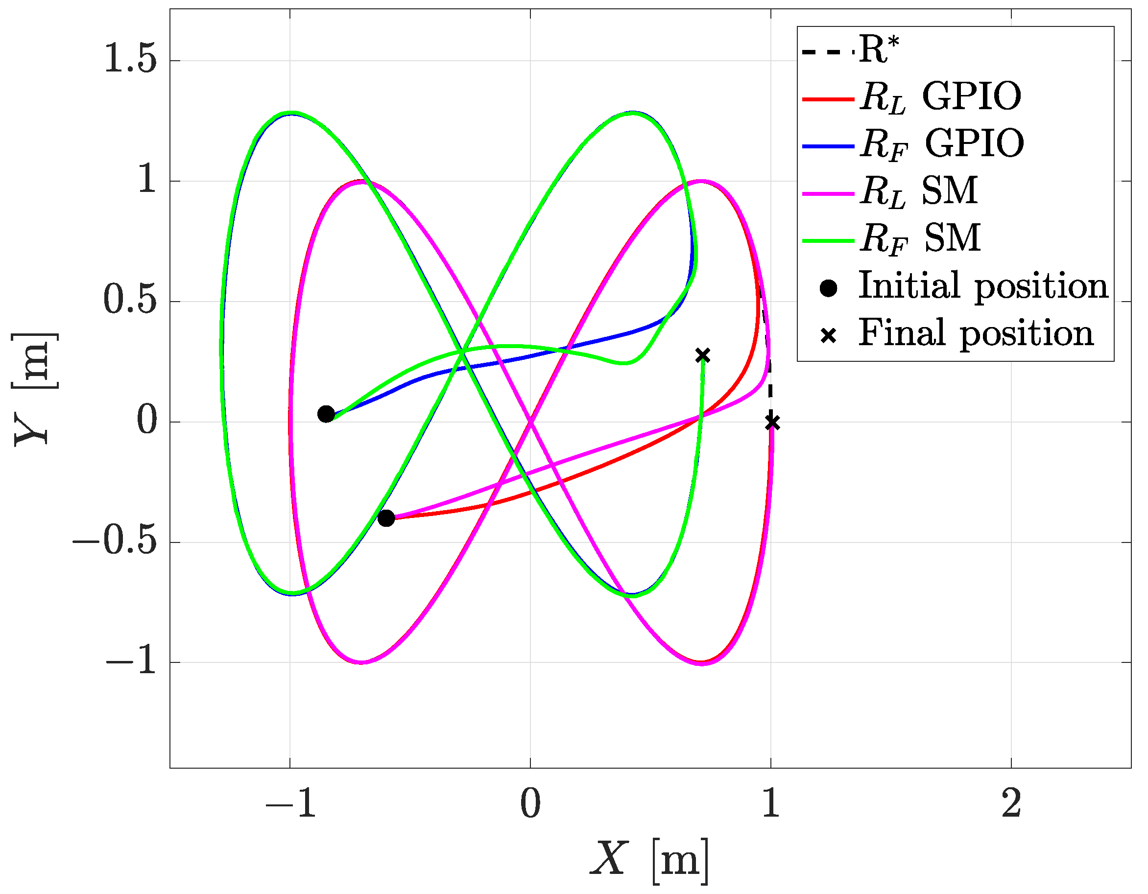
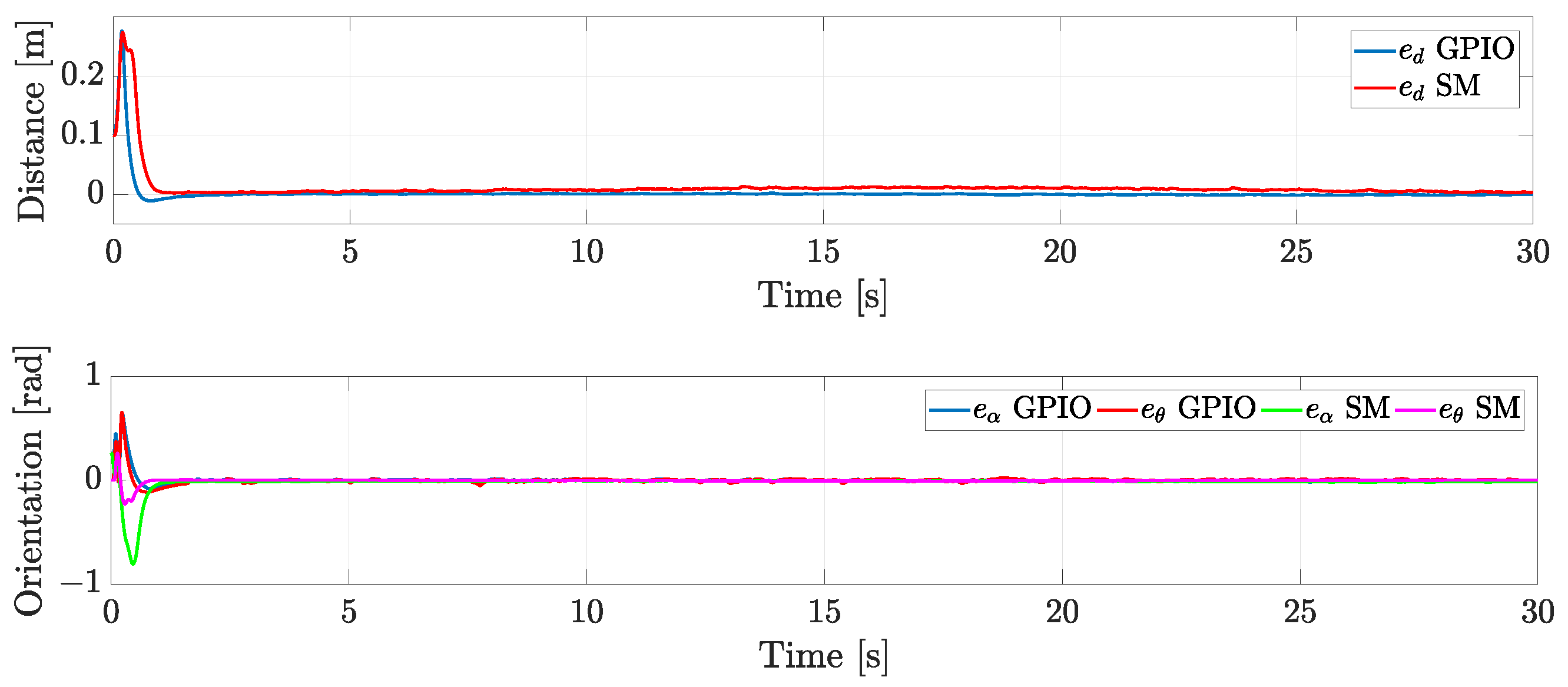
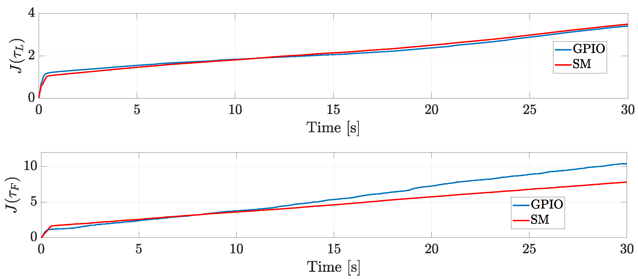
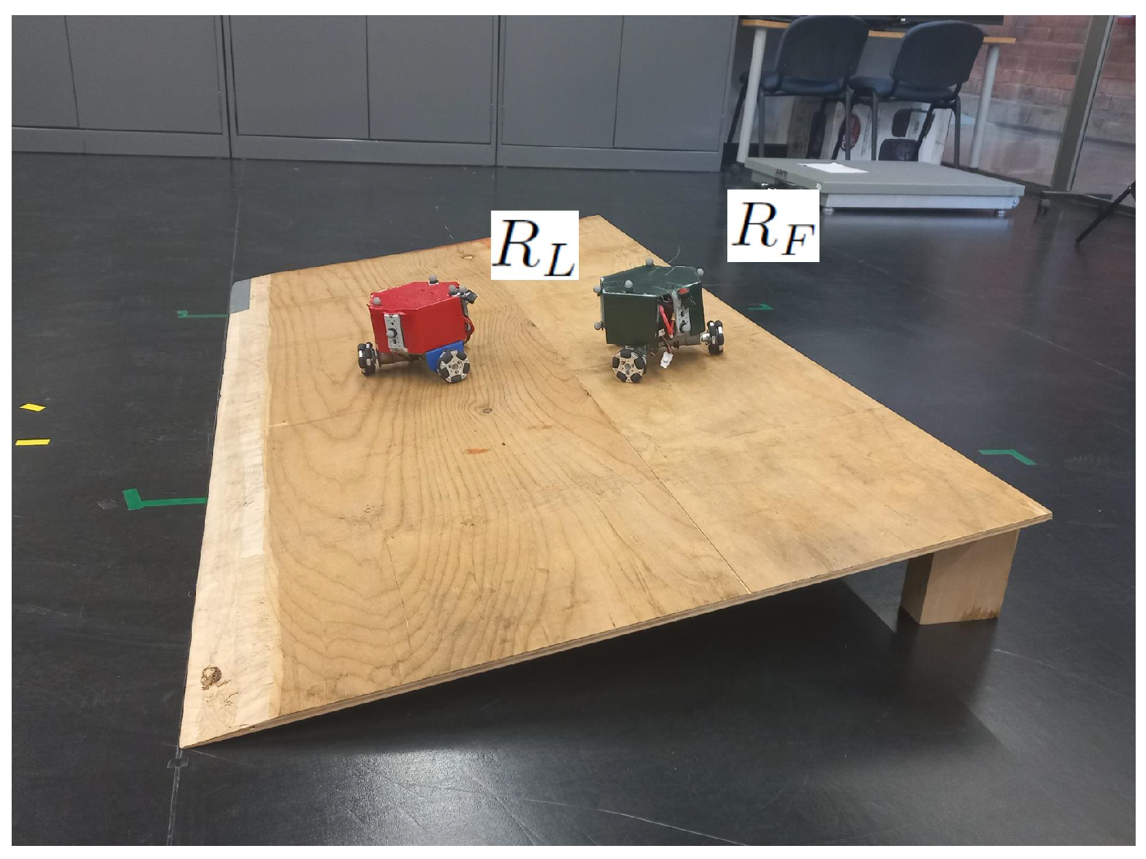
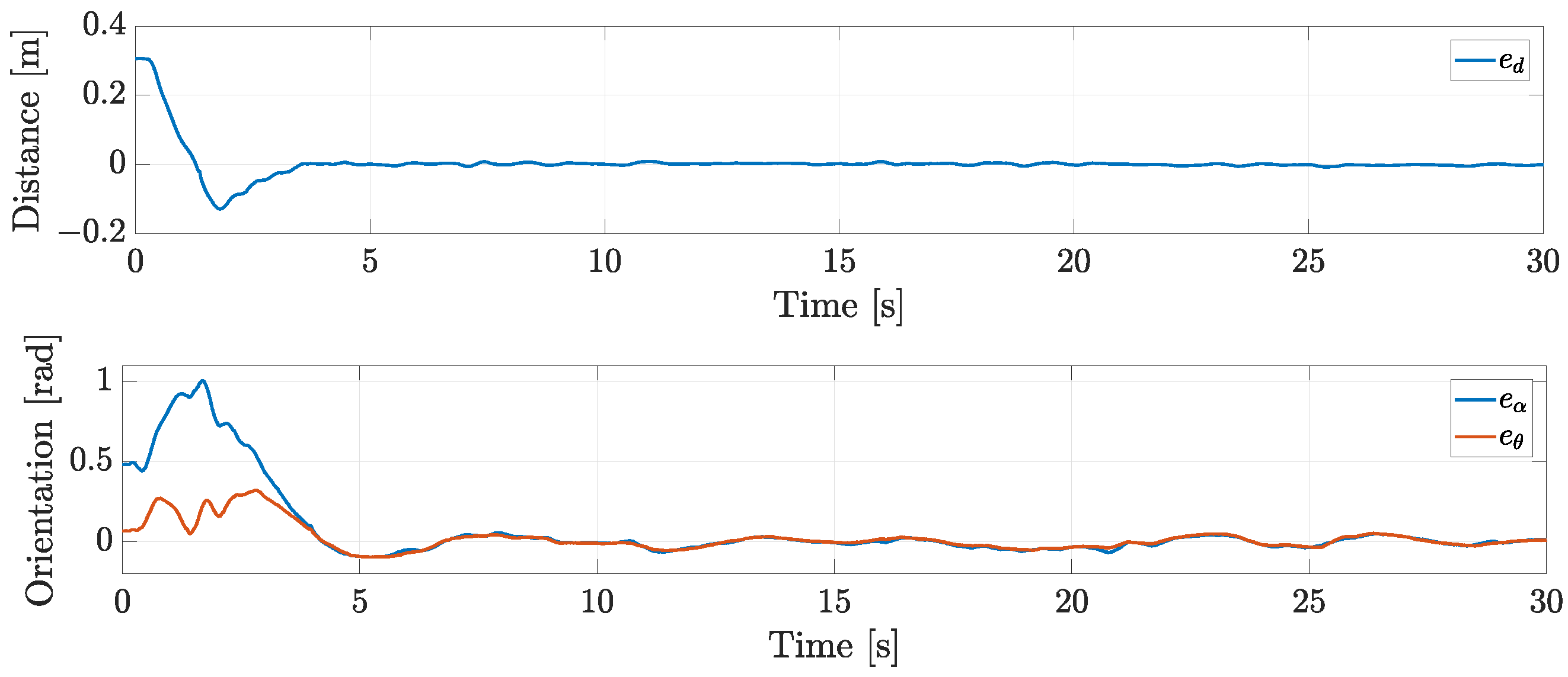
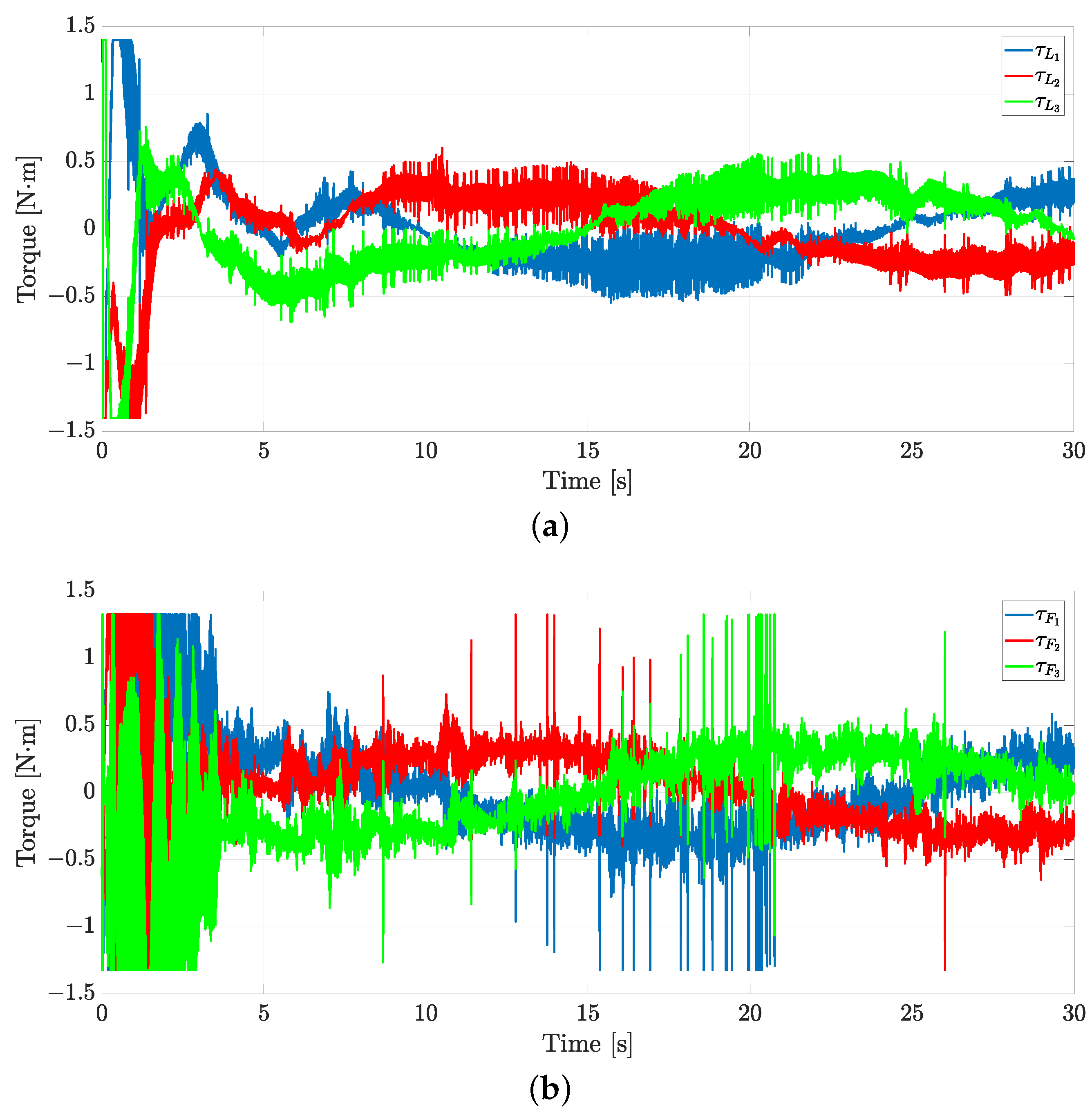
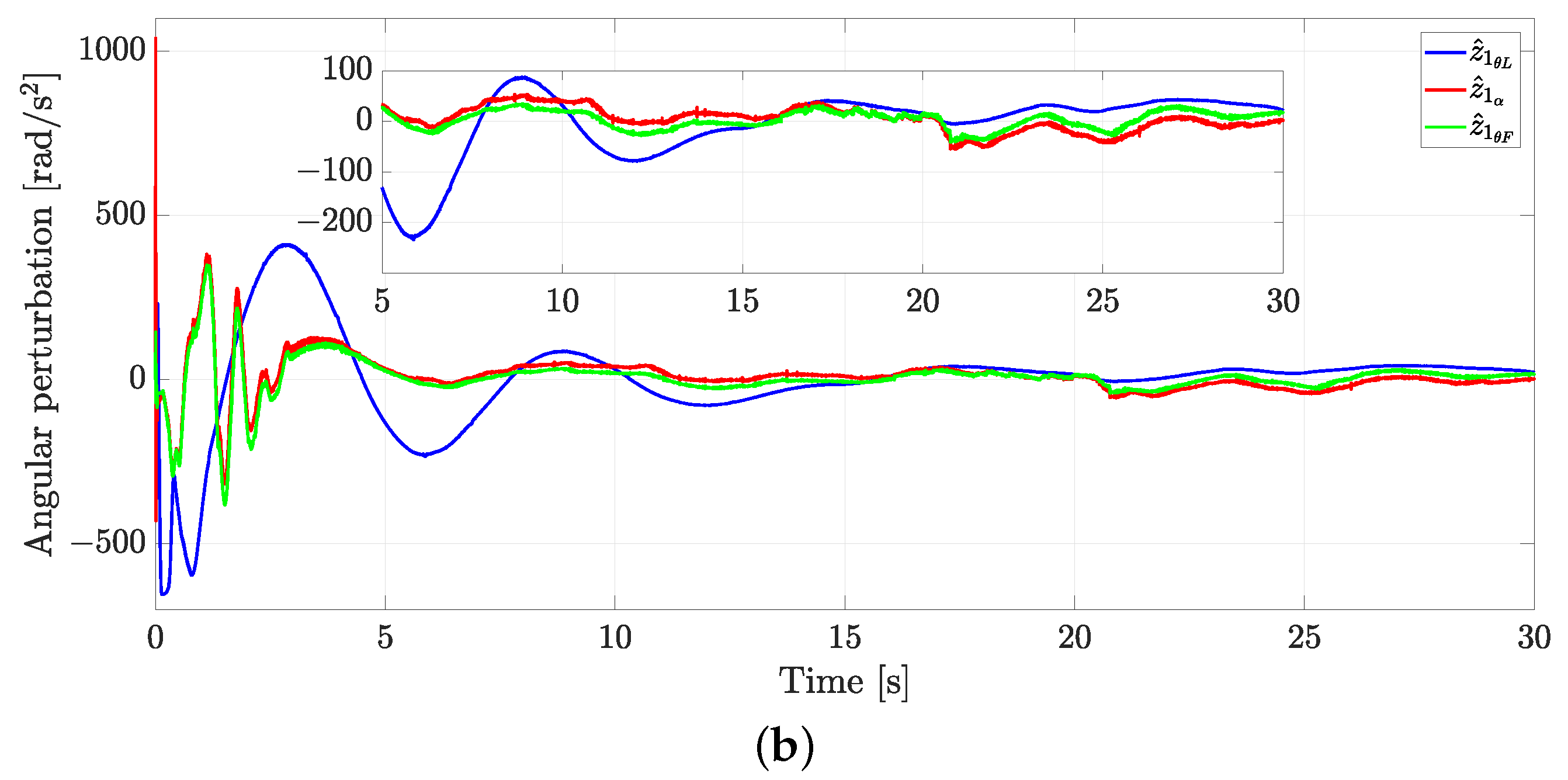
5.2. Real-Time Experiments

Two omnidirectional mobile robots were constructed for real-time experiments. Each robot uses three 12V POLOLU 37D geared motors, with a gear ratio of 1:70, and an encoder with a resolution of 64 counts per revolution (see Figure 8). For data acquisition, an STM32F4 Discovery board is implemented. At the same time, the communication between the computer and the robot is performed in real-time using a publicly available “waijung1504” Matlab/Simulink^© library, using Bluetooth communication protocol which is programmed on ESP32 micro-controller with ARDUINO-ESPRESSIF (https://docs.espressif.com/projects/arduino-esp32/en/latest/api/bluetooth.html, (accessed on 14 August 2023)) as it is shown in Figure 9. An STM32F4 Discovery board received the torque reference of each motor, and using a nonlinear function approximate the conversion of torque to PWM, as follows:

$$PW{M}_i=72.7802{\tau }_i+10.917\mathrm{sign}\left({\tau }_i\right),i=1,...,3.$$

(22)

The first term of the Equation (22) is the conversion of torque to PWM, and the second term compensates the dead zone of the motor due to the gearbox.

The experiments were carried out indoors with 10 infrared VICON© Bonita cameras with a precision of $0.5$ mm [47], which measures the attitude of each robot in an area of $5\times 4$m${}^2$ and with a sampling time of $0.005$ s. For this purpose, each robot was placed with several reflective markers, which form different patterns and thus can be detected by the TRACKER© camera software.

The experiments have become a proof of concept to evaluate the control strategy’s performance. In this context, this is considered a previous step for further experimentation with onboard sensors.

Two tests are carried out. For the former, the robots move in a horizontal plane: the leader tracks a circular trajectory with $0.5$ m radius, while the follower maintains a desired distance and formation angle concerning the leader. In the latter, the robots are moving in a horizontal plane and in an inclined plane to evaluate the performance of the control strategy in the face of external disturbances. The robots’ parameters; the controller and observer gains; and the desired distance, formation angle, and orientation are the same as in the numerical simulation.

5.2.1. First Case Study

For the first experiment, the initial conditions are ${\mathbf{q}}_L\left(0\right)={\left[\begin{array}{ccc}0.8794& 0.0253& 0.2061\end{array}\right]}^{\top }$ and ${\mathbf{q}}_F\left(0\right)={\left[\begin{array}{ccc}0.6232& 0.6837& 0.0673\end{array}\right]}^{\top }$. The trajectory in the plane for both robots is in Figure 10, where the leader tracks the circular trajectory (red line). In contrast, the follower (blue line) maintains a desired distance and formation angle concerning the leader.

Figure 11 presents the distance, formation angle, and orientation errors between the two considered robots. Note that the errors are oscillating around zero, i.e., the desired distance $d_{LF}\approx d_{LF}^{*}=0.4$ m, ${\alpha }_{LF}\approx {\alpha }_{LF}^{*}=\frac{\pi }{4}$ rad, and ${\theta }_F\approx 0$ rad.

Figure 12 illustrates the control inputs required to perform the desired motion of the robots. These signals correspond to the torques of each wheel. Note that such controls have higher-frequency oscillations due to selected higher observer gains needed to accomplish the formation tracking with relatively high accuracy. Furthermore, it is evident at the beginning that the robots are far away from the desired trajectory, so the control inputs reach their maximum value. Recall that the torques are saturated as ${\mathit{\tau }}_s\in \left[-1.4,1.4\right]$N·m.

The linear and angular velocities are shown in Figure 13a,b, respectively. Such velocities are calculated by taking the derivative of the position signals and adding a first-order Butterworth lowpass filter with a cutoff frequency of $12\pi$ rad/s. Considering that the velocities of the robots are bounded by $\pm 0.8$ m/s, and the angular velocity is bounded by $\pm 2\pi$ rad/s, one can note that such velocities remain inside the allowed values.

Figure 14 depicts the disturbance estimation for the leader and the follower robot. Specifically, Figure 14a presents the estimation of the linear disturbances. In the same context, Figure 14b estimates the angular disturbances. Note that such perturbations have a great magnitude initially. This comes from the fact that the robots are far away from the desired initial conditions.

5.2.2. Second Case Study

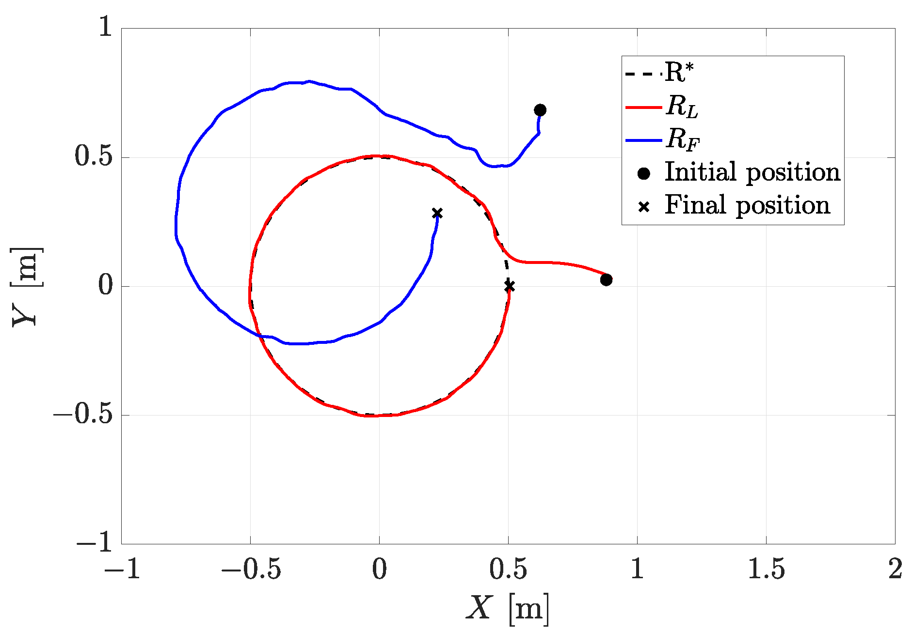
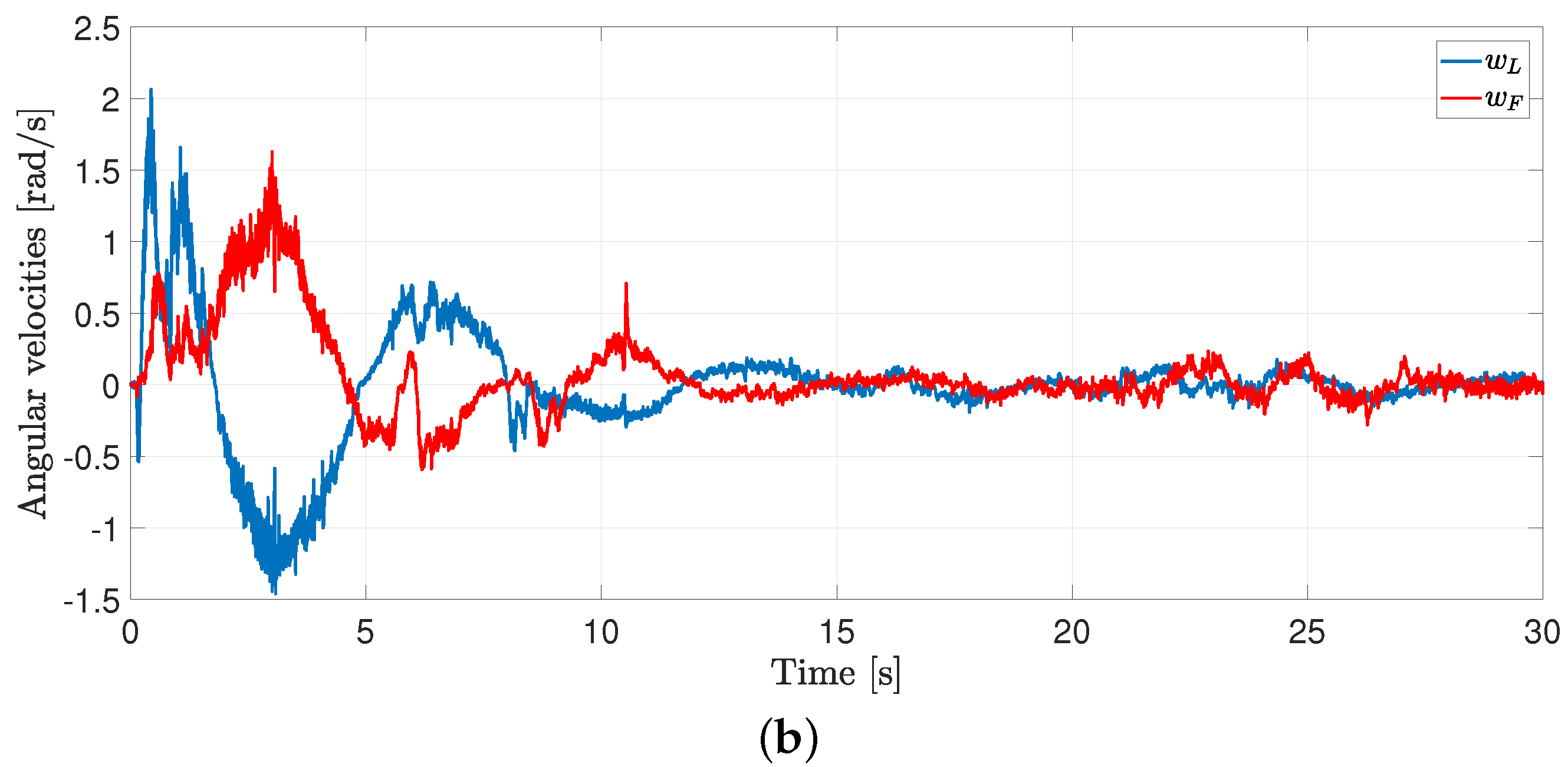
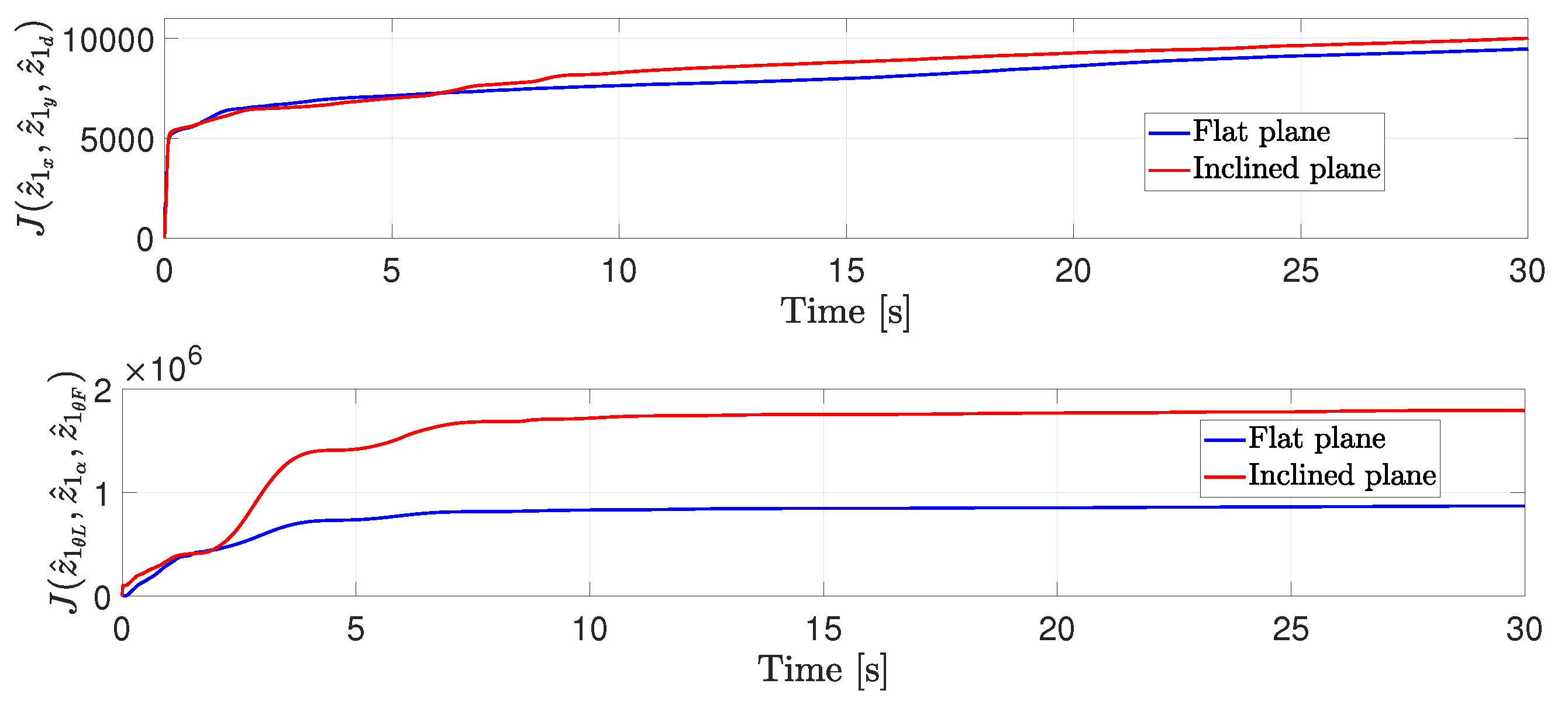
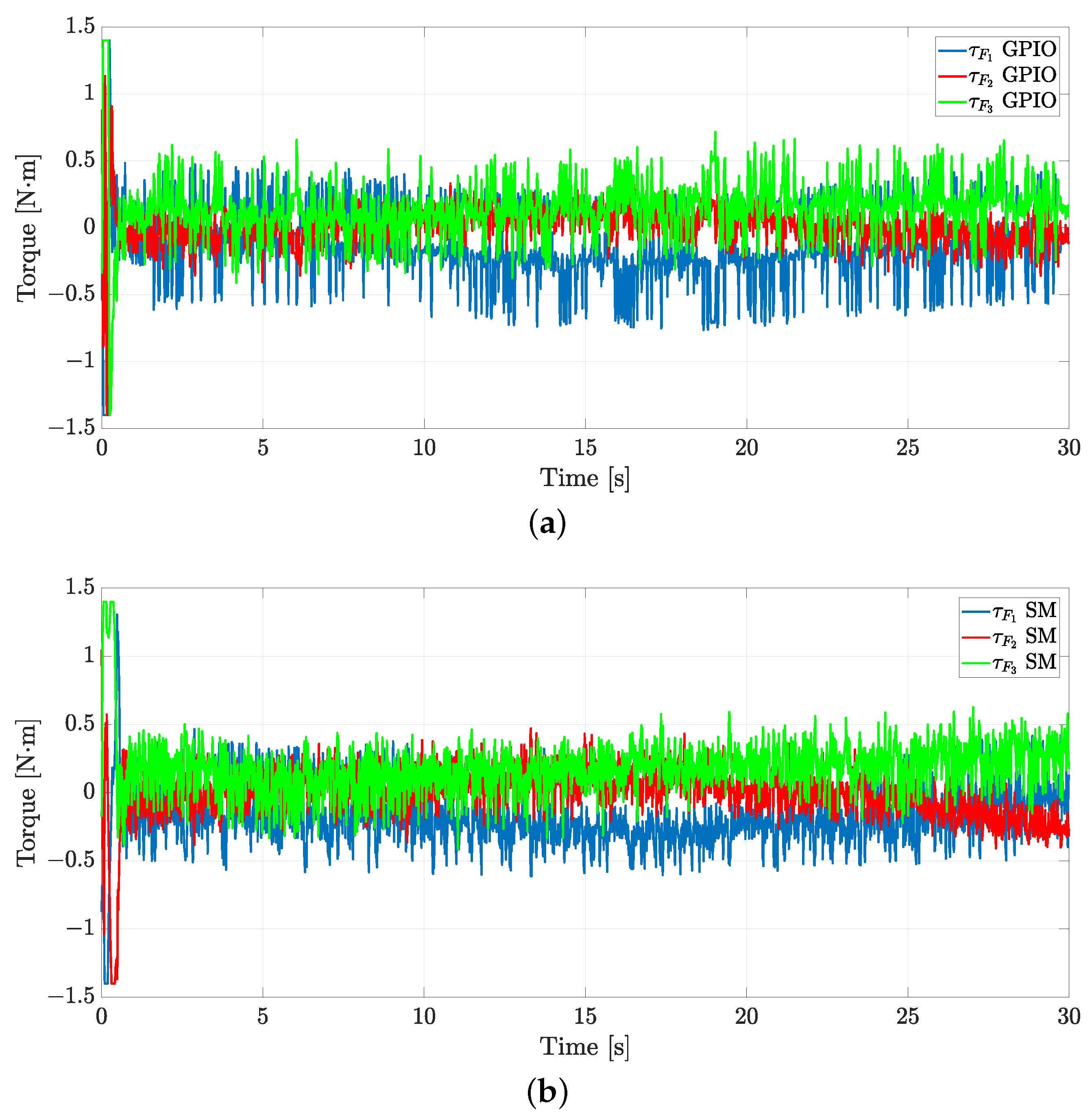
A second experiment was performed to verify the effectiveness of the proposed approach against unknown perturbations. In this sense, a platform with a tilt angle of 10 deg, as shown in Figure 8, is used as an unmodeled disturbance for both robots. The resultant motion of the robots is shown in Figure 15, from which one can note that the formation tracking is achieved regardless of the added perturbing surface tilt.

The distance, formation angle, and orientation errors are shown in Figure 16, where it is clear that the errors are oscillating around zero, i.e., the desired distance $d_{LF}\approx d_{LF}^{*}=0.4$m, ${\alpha }_{LF}\approx {\alpha }_{LF}^{*}=\frac{\pi }{4}$ rad, and ${\theta }_F\approx 0$ rad.

Figure 17 depicts the control inputs required to perform the desired robot motion. The robots are moving up the inclined plane when $t\in \left[5,28\right]$ s. Note that the control inputs have more oscillations than Figure 12. This is due to the disturbance produced by the inclined plane.

The linear and angular velocities are shown in Figure 18a,b, respectively. Again, note that such velocities remain inside the allowed values.

Finally, Figure 19 illustrates the disturbance estimation. It is essential to point out that the estimated disturbances differ from those presented in Figure 14. This is due to the presence of the inclined plane. Furthermore, the disturbances increase when the robots start their motion on the inclined plane.

A video of the experimental results can be watched at https://drive.google.com/drive/folders/11An29_Zuc_F4muxO2tVcYAg3e8qg5v0_?usp=sharing.

5.3. Discussion

To assess the overall performance, the same quadratic control index, presented in the numerical simulation, is used to compare the performance of the proposed technique in both scenarios. Furthermore, a quadratic observer index is defined as

$$\begin{array}{c}J({\widehat{z}}_{1_x},{\widehat{z}}_{1_y},{\widehat{z}}_{1_d})={\int }_0^t\left[{\widehat{z}}_{1_x}^2\left(\overline{\tau }\right)+{\widehat{z}}_{1_y}^2\left(\overline{\tau }\right)+{\widehat{z}}_{1_d}^2\left(\overline{\tau }\right)\right]\left(\overline{\tau }\right)d,\\ J({\widehat{z}}_{1_{\theta L}},{\widehat{z}}_{1_{\alpha }},{\widehat{z}}_{1_{\theta F}})={\int }_0^t\left[{\widehat{z}}_{1_{\theta L}}^2\left(\overline{\tau }\right)+{\widehat{z}}_{1_{\alpha }}^2\left(\overline{\tau }\right)+{\widehat{z}}_{1_{\theta F}}^2\left(\overline{\tau }\right)\right]d\overline{\tau }.\end{array}$$

As Figure 20 shows, it is clear that more energy is needed when the robots are moving in the inclined plane.

In a similar context, Figure 21 depicts that the estimated linear and angular perturbations increase when the robots move in the inclined plane. Based on those mentioned earlier, one concludes that even though the estimated perturbations are different, the control strategy can deal with them, and the robots can achieve tracking and formation control.

6. Conclusions and Future Work

This work developed a perturbed dynamic model based on the distance and the formation angle between a pair of omnidirectional mobile robots. The proposed control strategy needed information on the position, distance, and formation angle measurements while dedicated observers estimated the disturbances. From a mathematical point of view, it was proven that the tracking trajectory error of the leader converges asymptotically to zero. At the same time, the distance and formation angle errors also converge to zero, meaning the follower robot can maintain the desired distance and formation angle concerning the leader robot. The numerical simulation comparison of the proposed strategy with an SM controller shows that our control law can achieve smaller distance and formation angle errors than the SM approach. In the same context, real-time experiments validate the performance of the proposed control strategy in terms of accuracy and robustness, even when the robots needed to perform their given tasks under perturbing phenomena.

For further research, different tests will be carried out to determine (a) how fast the robots can be moving and (b) the performance of the robots for different trajectories where the centripetal/centrifugal acceleration changes both in magnitude and direction. On the other hand, we will tackle the time-varying formation control based on the distance and formation angle for a heterogeneous multi-agent system in a group of n robots, its implementation in cyber-physical multi-robot formations, and onboard sensors.

References

1. Kagan, E.; Shvalb, N.; Ben-Gal, I. Autonomous Mobile Robots and Multi-Robot Systems: Motion-Planning, Communication, and Swarming; John Wiley & Sons: Hoboken, NJ, USA, 2019. [Google Scholar]
2. Farrugia, J.L.; Fabri, S.G. Swarm Robotics for Object Transportation. In Proceedings of the 2018 UKACC 12th International Conference on Control (CONTROL), Sheffield, UK, 5–7 September 2018; pp. 353–358. [Google Scholar] [CrossRef]
3. Mouradian, C.; Sahoo, J.; Glitho, R.H.; Morrow, M.J.; Polakos, P.A. A coalition formation algorithm for Multi-Robot Task Allocation in large-scale natural disasters. In Proceedings of the International Wireless Communications and Mobile Computing Conference, Valencia, Spain, 26–30 June 2017; pp. 1909–1914. [Google Scholar] [CrossRef]
4. Queralta, J.P.; Taipalmaa, J.; Can Pullinen, B.; Sarker, V.K.; Nguyen Gia, T.; Tenhunen, H.; Gabbouj, M.; Raitoharju, J.; Westerlund, T. Collaborative Multi-Robot Search and Rescue: Planning, Coordination, Perception, and Active Vision. IEEE Access 2020, 8, 191617–191643. [Google Scholar] [CrossRef]
5. Hernandez-Martinez, E.G.; Foyo-Valdes, S.A.; Puga-Velazquez, E.S.; Meda-Campaña, J.A. Hybrid Architecture for Coordination of AGVs in FMS. Int. J. Adv. Robot. Syst. 2014, 11, 41. [Google Scholar] [CrossRef]
6. Wicaksono, H.; Nilkhamhang, I. Glocal controller-based formation control strategy for flexible material handling. In Proceedings of the 2017 56th Annual Conference of the Society of Instrument and Control Engineers of Japan (SICE), Kanazawa, Japan, 19-22 September 2017; pp. 787–792. [Google Scholar] [CrossRef]
7. Schwager, M.; Vitus, M.P.; Powers, S.; Rus, D.; Tomlin, C.J. Robust Adaptive Coverage Control for Robotic Sensor Networks. IEEE Trans. Control. Netw. Syst. 2017, 4, 462–476. [Google Scholar] [CrossRef]
8. Miah, M.S.; Knoll, J. Area Coverage Optimization Using Heterogeneous Robots: Algorithm and Implementation. IEEE Trans. Instrum. Meas. 2018, 67, 1380–1388. [Google Scholar] [CrossRef]
9. Hernandez-Martinez, E.G.; Ferreira-Vazquez, E.D.; Fernandez-Anaya, G.; Flores-Godoy, J.J. Formation tracking of heterogeneous mobile agents using distance and area constraints. Complexity 2017, 2017, 9404193. [Google Scholar] [CrossRef]
10. Kamel, M.A.; Yu, X.; Zhang, Y. Formation control and coordination of multiple unmanned ground vehicles in normal and faulty situations: A review. Annu. Rev. Control. 2020, 49, 128–144. [Google Scholar] [CrossRef]
11. Oh, K.K.; Park, M.C.; Ahn, H.S. A survey of multi-agent formation control. Automatica 2015, 53, 424–440. [Google Scholar] [CrossRef]
12. Wang, W.; Huang, J.; Wen, C.; Fan, H. Distributed adaptive control for consensus tracking with application to formation control of nonholonomic mobile robots. Automatica 2014, 50, 1254–1263. [Google Scholar] [CrossRef]
13. Zou, Y.; Wen, C.; Guan, M. Distributed Adaptive Control for Distance-based Formation and Flocking control of Multi-Agent Systems. IET Control. Theory Appl. 2019, 13, 878–885. [Google Scholar] [CrossRef]
14. Wang, Y.; Hussein, I.I. Search and Classification Using Multiple Autonomous Vehicles; Springer: London, UK, 2012. [Google Scholar] [CrossRef]
15. Su, Y.; Shi, P.; Wang, X.; Xu, D. Leader-following rendezvous for single-integrator multi-agent systems with uncertain leader. In Proceedings of the 2017 11th Asian Control Conference (ASCC), Gold Coast, QLD, Australia, 17–20 December 2017; pp. 162–167. [Google Scholar] [CrossRef]
16. Cruz-Ancona, C.D.; Martínez-Guerra, R.; Pérez-Pinacho, C.A. A leader-following consensus problem of multi-agent systems in heterogeneous networks. Automatica 2020, 115, 108899. [Google Scholar] [CrossRef]
17. Miao, Z.; Liu, Y.H.; Wang, Y.; Yi, G.; Fierro, R. Distributed Estimation and Control for Leader-Following Formations of Nonholonomic Mobile Robots. IEEE Trans. Autom. Sci. Eng. 2018, 15, 1946–1954. [Google Scholar] [CrossRef]
18. Yan, L.; Ma, B. Practical Formation Tracking Control of Multiple Unicycle Robots. IEEE Access 2019, 7, 113417–113426. [Google Scholar] [CrossRef]
19. Taheri, H.; Zhao, C.X. Omnidirectional mobile robots, mechanisms and navigation approaches. Mech. Mach. Theory 2020, 153, 103958. [Google Scholar] [CrossRef]
20. Paniagua Contro, P.; Hernandez-Martinez, E.; González-Medina, O.; González-Sierra, J.; Flores-Godoy, J.J.; Ferreira, E.; Fernandez-Anaya, G. Extension of Leader-Follower Behaviours for Wheeled Mobile Robots in Multirobot Coordination. Math. Probl. Eng. 2019, 2019, 4957259. [Google Scholar] [CrossRef]
21. Roza, A.; Maggiore, M.; Scardovi, L. A Smooth Distributed Feedback for Formation Control of Unicycles. IEEE Trans. Autom. Control. 2019, 64, 4998–5011. [Google Scholar] [CrossRef]
22. Tang, X.; Ji, Y.; Gao, F.; Zhao, C. Research on multi-robot formation controlling method. In Proceedings of the Third International Conference on Cyberspace Technology (CCT 2015), Beijing, China, 17–18 October 2015; pp. 1–3. [Google Scholar] [CrossRef]
23. Morbidi, F.; Bretagne, E. A New Characterization of Mobility for Distance-Bearing Formations of Unicycle Robots. In Proceedings of the 2018 IEEE/RSJ International Conference on Intelligent Robots and Systems (IROS), Madrid, Spain, 1–5 October 2018; pp. 4833–4839. [Google Scholar] [CrossRef]
24. González-Sierra, J.; Flores-Montes, D.; Hernandez-Martinez, E.G.; Fernández-Anaya, G.; Paniagua-Contro, P. Robust circumnavigation of a heterogeneous multi-agent system. Auton. Robot. 2021, 45, 265–281. [Google Scholar] [CrossRef]
25. Manel, M.; Faouzi, B. Predictive control based on dynamic modeling of omnidirectional mobile robot. In Proceedings of the International Conference on Engineering & MIS, Monastir, Tunisia, 8–10 May 2017; pp. 1–6. [Google Scholar] [CrossRef]
26. Soltani, N.; Shahmansoorian, A.; Khosravi, M. Robust distance-angle leader-follower formation control of non-holonomic mobile robots. In Proceedings of the 2014 2nd RSI/ISM International Conference on Robotics and Mechatronics, ICRoM 2014, Tehran, Iran, 15–17 October 2014; pp. 24–28. [Google Scholar] [CrossRef]
27. Sun, Z.; Mou, S.; Deghat, M.; Anderson, B.D.O. Finite time distributed distance-constrained shape stabilization and flocking control for d-dimensional undirected rigid formations. Int. J. Robust Nonlinear Control 2016, 26, 2824–2844. [Google Scholar] [CrossRef]
28. Oh, K.K.; Ahn, H.S. Distance-based undirected formations of single-integrator and double-integrator modeled agents in n-dimensional space. Int. J. Robust Nonlinear Control 2014, 24, 1809–1820. [Google Scholar] [CrossRef]
29. Yang, Z.; Li, S.; Xu, H.; Yu, D.; Wang, Z.; Philip Chen, C. Formation Control of Omnidirectional Mobile Robots Based on Bionic Coupling Mechanism. In Proceedings of the 2021 IEEE International Conference on Unmanned Systems (ICUS), Beijing, China, 15–17 October 2021; pp. 184–189. [Google Scholar] [CrossRef]
30. Abhishek, V.; Saha, S.K. Dynamic identification and model based control of an omni-wheeled mobile robot. In Proceedings of the International Conference on Robotics and Mechatronics, Tehran, Iran, 26–28 October 2016; pp. 595–600. [Google Scholar] [CrossRef]
31. Rezazadegan, F.; Shojaei, K.; Sheikholeslam, F.; Chatraei, A. A novel approach to 6-DOF adaptive trajectory tracking control of an AUV in the presence of parameter uncertainties. Ocean Eng. 2015, 107, 246–258. [Google Scholar] [CrossRef]
32. Elhaki, O.; Shojaei, K. Robust saturated dynamic surface controller design for underactuated fast surface vessels including actuator dynamics. Ocean Eng. 2021, 229, 108987. [Google Scholar] [CrossRef]
33. Qin, J.; Du, J. Minimum-learning-parameter-based adaptive finite-time trajectory tracking event-triggered control for underactuated surface vessels with parametric uncertainties. Ocean Eng. 2023, 271, 113634. [Google Scholar] [CrossRef]
34. Bai, H.; Yu, B.; Gu, W. Research on Position Sensorless Control of RDT Motor Based on Improved SMO with Continuous Hyperbolic Tangent Function and Improved Feedforward PLL. J. Mar. Sci. Eng. 2023, 11. [Google Scholar] [CrossRef]
35. Qin, J.; Du, J.; Li, J. Adaptive Finite-Time Trajectory Tracking Event-Triggered Control Scheme for Underactuated Surface Vessels Subject to Input Saturation. IEEE Trans. Intell. Transp. Syst. 2023, 24, 8809–8819. [Google Scholar] [CrossRef]
36. Radke, A.; Gao, Z. A survey of state and disturbance observers for practitioners. In Proceedings of the American Control Conference, Minneapolis, MN, USA, 14–16 June 2006. [Google Scholar] [CrossRef]
37. Madonski, R.; Herman, P. Survey on methods of increasing the efficiency of extended state disturbance observers. ISA Trans. 2015, 56, 18–27. [Google Scholar] [CrossRef] [PubMed]
38. Łakomy, K.; Patelski, R.; Pazderski, D. ESO Architectures in the Trajectory Tracking ADR Controller for a Mechanical System: A Comparison. In Advanced, Contemporary Control; Bartoszewicz, A., Kabziński, J., Kacprzyk, J., Eds.; Springer: Berlin/Heidelberg, Germany, 2020; pp. 1323–1335. [Google Scholar] [CrossRef]
39. Wu, H.L.; Tsai, C.C.; Tai, F.C. Integral Terminal Sliding-Mode Formation Control for Uncertain Heterogeneous Networked Mecanum-Wheeled Omnidirectional Robots. In Proceedings of the IEEE International Conference on Systems, Man, and Cybernetics, Miyazaki, Japan, 7–10 October 2018; pp. 1815–1820. [Google Scholar] [CrossRef]
40. Fu, H.; Li, Y.; Wang, Y.; Zhang, Z. Omnidirectional Mobile Robot Active Disturbance Rejection Control. In Proceedings of the IEEE International Conference on Mechatronics and Automation, Changchun, China, 5–8 August 2018; pp. 227–232. [Google Scholar] [CrossRef]
41. Sira-Ramírez, H.; Castro-Linares, R.; Puriel-Gil, G. An Active Disturbance Rejection Approach to Leader-Follower Controlled Formation. Asian J. Control 2014, 16, 382–395. [Google Scholar] [CrossRef]
42. Ramírez-Neria, M.; Luviano-Juárez, A.; Madonski, R.; Ramírez-Juárez, R.; Lozada-Castillo, N.; Gao, Z. Leader-Follower ADRC Strategy for Omnidirectional Mobile Robots without Time-Derivatives in the Tracking Controller. In Proceedings of the American Control Conference, San Diego, CA, USA, 31 May–2 June 2023; pp. 405–410. [Google Scholar] [CrossRef]
43. Sira-Ramirez, H.; Luviano-Juárez, A.; Ramírez-Neria, M.; Zurita-Bustamante, E.W. Active Disturbance Rejection Control of Dynamic Systems: A Flatness Based Approach; Butterworth-Heinemann: Oxford, UK, 2017. [Google Scholar] [CrossRef]
44. Han, J. From PID to active disturbance rejection control. IEEE Trans. Ind. Electron. 2009, 56, 900–906. [Google Scholar] [CrossRef]
45. Sira-Ramírez, H.; Ramírez-Neria, M.; Rodríguez-Angeles, A. On the linear control of nonlinear mechanical systems. In Proceedings of the IEEE Conference on Decision and Control, Atlanta, GA, USA, 15-17 December 2010; pp. 1999–2004. [Google Scholar] [CrossRef]
46. Gao, Z. Scaling and bandwidth-parameterization based controller tuning. In Proceedings of the American Control Conference, Denver, CO, USA, 4–6 June 2003; pp. 4989–4996. [Google Scholar] [CrossRef]
47. Scoz, R.D.; Espindola, T.R.; Santiago, M.F.; de Oliveira, P.R.; Alves, B.M.O.; Ferreira, L.M.A.; Amorim, C.F. Validation of a 3D Camera System for Cycling Analysis. Sensors 2021, 21, 4473. [Google Scholar] [CrossRef]
Figure 1. Schematic diagram of the considered leader–follower setup with used notation.
Robotics 12 00122 g001
Figure 2. Simulation: comparison of robot trajectories in a 2D plane.
Robotics 12 00122 g002
Figure 3. Simulation: comparison of the distance error, the formation angle error, and the orientation error.
Robotics 12 00122 g003
Figure 4. Simulation: comparison of the leader’s control inputs. (a) Control inputs for the leader with the GPIO. (b) Control inputs for the leader with the SM.
Robotics 12 00122 g004
Figure 5. Simulation: Comparison of the follower’s control inputs. (a) Control inputs for the follower with the GPIO. (b) Control inputs for the follower with the SM.
Robotics 12 00122 g005
Figure 6. Simulation: comparison of the quadratic error index.
Robotics 12 00122 g006
Figure 7. Simulation: comparison of the quadratic control inputs.
Robotics 12 00122 g007
Figure 8. The omnidirectional mobile robots (leader R L and follower R F ) used in the experiments.
Robotics 12 00122 g008
Figure 9. Robot prototype communication and low-level power electronics control.
Robotics 12 00122 g009
Figure 10. Exp1: robots’ trajectories in 2D plane.
Robotics 12 00122 g010
Figure 11. Exp1: distance, formation angle, and orientation errors.
Robotics 12 00122 g011
Figure 12. Exp1: control inputs for the two robots. (a) Control inputs for the leader. (b) Control inputs for the follower.
Robotics 12 00122 g012
Figure 13. Exp1: linear and angular velocities for both robots. (a) Linear velocities for both robots. (b) Angular velocities for both robots.
Robotics 12 00122 g013
Figure 14. Exp1: disturbance estimation using GPIO. (a) Linear disturbance estimation. (b) Angular disturbance estimation.
Robotics 12 00122 g014aRobotics 12 00122 g014b
Figure 15. Exp2: robots’ trajectories in 3D plane.
Robotics 12 00122 g015
Figure 16. Exp2: Distance, formation angle, and orientation errors.
Robotics 12 00122 g016
Figure 17. Exp2: control inputs for the two robots. (a) Control inputs for the leader. (b) Control inputs for the follower.
Robotics 12 00122 g017
Figure 18. Exp2: linear and angular velocities for both robots. (a) Linear velocities for both robots. (b) Angular velocities for both robots.
Robotics 12 00122 g018aRobotics 12 00122 g018b
Figure 19. Exp2: disturbance estimation using GPIO. (a) Linear disturbance estimation. (b) Angular disturbance estimation.
Robotics 12 00122 g019
Figure 20. Comparison of the quadratic control inputs.
Robotics 12 00122 g020
Figure 21. Comparison of the quadratic estimated linear and angular perturbations.
Robotics 12 00122 g021
Disclaimer/Publisher’s Note: The statements, opinions and data contained in all publications are solely those of the individual author(s) and contributor(s) and not of MDPI and/or the editor(s). MDPI and/or the editor(s) disclaim responsibility for any injury to people or property resulting from any ideas, methods, instructions or products referred to in the content.