1. Introduction
As robotic technologies have developed, the autonomous capabilities of robots have greatly improved, with robots now able to navigate through complex environments and avoid both static and dynamic obstacles. With the advent of these capabilities, the potential application areas of robots have expanded far beyond the controlled manufacturing environments where robots were first used. Autonomous navigation strategies have been developed which allow robots to complete pre-defined tasks in uncontrolled and changing environments, such as navigating to a specific target location and even tracking a target through an environment. However, existing technologies require prior knowledge to complete such tasks, such as knowing the target location a priori.
Some potential applications for autonomous robots include fire rescue, in-home emergency medical response, and object retrieval in hazardous environments. The characteristic that all of these applications have in common is that the task is not well-defined a priori because the target location for the robot may be unknown at initiation of the task. In the case of fire rescue, the robot must navigate through a burning building to a person trapped inside, but the location of this person within the building may be unknown. For emergency medical response, the robot must respond to the occurrence of an adverse medical event and to do so must first navigate to the patient who could be located anywhere within their home. The precise locations of objects in hazardous environments may not be known, and thus the robot must determine the location of the desired object to be able to perform the retrieval task. These examples of applications for autonomous robots illustrate that the task cannot be fully defined a priori, meaning part of the task for the robot is to determine the location of the target in real time to navigate to the target and complete the task. Thus, in this paper we focus on the challenge of autonomous target localization in indoor environments for robotic tasks where the location of the target is unknown. In
Section 2, the problem is presented and key characteristics of a good solution are identified.
Section 3 reviews existing technologies related to indoor target localization for various applications.
Section 4 introduces the proposed Bluetooth homing controller solution, and
Section 5 provides details of the structure and implementation of the controller.
Section 6 and
Section 7 provide a description of the simulation experiments used to validate the homing controller algorithm and the simulation results. A brief summary of preliminary hardware implementation is provided in
Section 8, followed by a discussion and conclusions in
Section 9 and
Section 10.
2. Problem Statement
Target localization is a challenge that has not been widely addressed in autonomous robotic navigation tasks, especially for indoor environments. Target localization refers to determining the location of a specified object of interest in an environment. For autonomous robotics, this means determining the target location to which a robot must navigate to complete a task, in the case where this target location is unknown a priori. Target localization is a different problem than robot localization, which refers to determining the location of a robot within its environment. Robot localization has been studied much more extensively than target localization, but many solutions for robot localization use expensive sensors and environment infrastructure, which make these solutions infeasible for application to target localization. In outdoor environments, global positioning system (GPS) is commonly used for target localization. However, GPS is unable to provide sufficient accuracy in indoor environments to be suitable for most applications. The solution to the indoor target localization task must satisfy four mandatory characteristics: (i) operates in scenarios where there is not a clear line of sight to the target object; (ii) provides a means of object-specific ID for the target; (iii) does not require existing infrastructure in the environment to operate; (iv) integrates with existing autonomous navigation technologies to create a comprehensive solution providing localization of and navigation to a target. In order to achieve the criteria of object-specific ID, the solution will require that the target object is equipped with some kind of beacon for identification. The objective is that this beacon can be identified and localized using only a sensor mounted on the mobile robot, without the need for any additional sensors or environmental information. Additional characteristics of the solution that are desirable include low energy consumption of both the beacon and the sensor, target localization accuracy of under 0.2 m, and a widely available technology for ease of deployment.
3. Existing Solutions
Sensor technologies that are commonly used in autonomous navigation tasks include light detection and ranging (LIDAR) and ultrasonic (US) sensors. These are used for environment mapping and obstacle avoidance as they measure the distance to obstacles along a measurement direction. However, neither of these technologies is suitable for the proposed challenge because they do not satisfy all necessary criteria to complete the task. Both LIDAR and US are line-of-sight sensors, meaning that they only provide distance readings to the first obstacle that is encountered along the direction of sensing. These technologies provide no means of object-specific identification, in addition to requiring a line of sight to the object, thus eliminating these technologies as possible solutions. Cameras can be used with computer vision (CV) for object identification and localization [
1], but this solution also requires a line of sight to the object. Additionally, while CV may be able to identify the type of object that is the target, it may be unable to distinguish between multiples of the same type of object when a specific one is needed.
Radio frequency identification (RFID) satisfies the object-specific ID criteria, can be used when there is not a clear line of sight to the target, and has been demonstrated as a solution for object tracking. Liu et al. used particle filtering with passive ultra-high-frequency (UHF) RFID tags for dynamic object tracking with a mobile robot. This approach was successful for dynamic object tracking except in cases where the RFID tag was affixed to a metal object and in cases of cluttered environments where line of sight to the target was quickly lost [
2]. Duan et al. used a fusion of RFID and CV to achieve 10.33 mm mean location tracking accuracy [
3], but this hybrid system requires line of sight for the CV component. These examples illustrate that RFID is a feasible method for target following when the target is within close range, but it has some deficiencies for target localization applications. Passive UHF RFID tags have a limited range (usually <12 m), making them unsuitable for applications where the target is far away, as the signal will be lost. Additionally, RFID is sensitive to environmental factors, such as metal objects, water, and even walls, which can greatly affect transmitting range. As such, the limitations of RFID tracking are prohibitive for use in a robust target localization system.
Another related area of research is the development of indoor positioning systems. These systems are commonly used for asset tracking and even localization of robots within an environment and employ technologies such as ultra-wideband (UWB) and Bluetooth. The general structure of these systems is to use static reference sensor locations, or anchors, within an environment, along with beacons fixed to the objects with desired tracking. The location of the tracked object can be estimated using readings from the anchors.
UWB technology is becoming more popular as a method for indoor robot localization because it provides relatively high accuracy and is easily scalable for multi-robot systems [
4]. A system for robot self-localization using UWB technology was presented by Ledergerber et al. [
5]. This system used three static anchors and timed difference of arrival to track the location of a quadrocoptor within an RMS error of 0.3 m. Cao et al. proposed a system using a single UWB anchor combined with a 9-DOF inertial measurement unit (IMU) for robot tracking, achieving an RMS tracking error of 0.48 m [
6]. For multi-robot localization applications, the most common framework uses fixed anchors which are used to localize all robots. Research is also being carried out using UWB for cooperative localization and to coordinate cooperative actions for multi-robot systems [
7].
For Bluetooth-based systems, much research was carried out before the introduction of Bluetooth 5.1 and relied on received signal strength indication (RSSI) to determine the proximity of two Bluetooth units [
8,
9,
10]. While these systems were successful at localization to a certain extent, it was found that the variability in RSSI limited the accuracy of such systems to the range of 1–2 m, which was above the acceptable error threshold in many applications.
The introduction of Bluetooth 5.1 direction-finding greatly expanded the capabilities of using Bluetooth for indoor localization. Bluetooth angle of arrival is an implementation of direction-finding using a transmitter, which is a beacon capable of emitting constant tone extension (CTE), and a receiver, which contains an antenna array to receive the CTE signal. The angle of arrival of the signal between the beacon and the antenna array can be calculated using IQ sampling (which contains phase information about the signal) delivered via the CTE. The phase difference between the signal at the different antennas on the array and the known geometry of the antenna array allow calculation of the angle of arrival [
11]. There is much ongoing research aimed at improving the accuracy of the angle estimation via various techniques, such a combination of nonlinear curve fitting, Kalman filtering, and Gaussian filtering [
12] and machine learning frameworks [
13].
Frameworks using Bluetooth AoA for indoor localization have exhibited varying results. Methods relying solely on AoA measurements have achieved mean accuracies of <1 m [
14,
15], but suffer from variable accuracy depending on beacon and antenna locations, in addition to line-of-sight and other interference reducing measurement accuracy. Additionally, a wide variance has been reported in the accuracy of AoA measurements, from a mean error of 1.9 degrees over the full 360-degree range in [
11], to a mean absolute error (MAE) of 29 degrees over a 180-degree range in [
16]. To address variations in AoA measurement accuracy, [
16] proposes a hybrid method of localization incorporating RSSI measurements to improve accuracy.
To the knowledge of the authors, little research has been carried out examining indoor target localization in the context of autonomous mobile robotic task execution. The existing research provides a framework for designing a system using Bluetooth or similar technologies for target localization. The proposed systems, however, rely on multiple reference sensors placed throughout the environment. Such a framework is not feasible for the applications presented in this paper, where modifications to the environment may not be possible. Thus, the system must function using only the robot-equipped sensors. Vasilopoulos et al. used an RF-range sensor to perform homing to an unknown target location for a legged robot, but details and performance of the target localization portion of the experiment were not provided [
17].
4. Proposed Solution
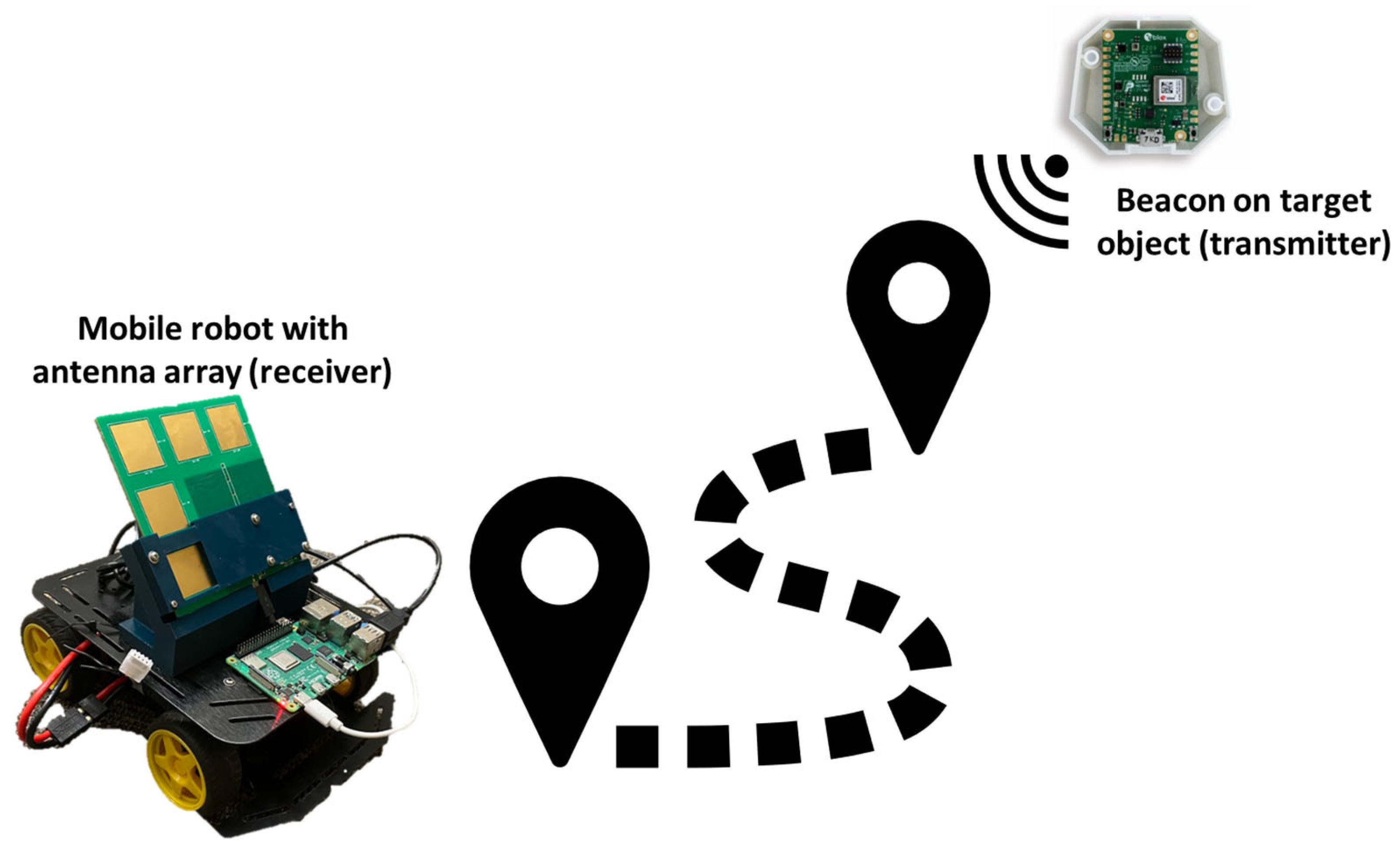
This paper proposes a method by which Bluetooth 5.1 Angle of Arrival (AoA) technology is used to create a homing controller performing real-time target localization. The controller uses Bluetooth signal between a mobile robot and target (of initially unknown location) to determine the precise target location as the autonomous robot navigates through the environment. In the proposed solution, a transmitting Bluetooth beacon is attached to the target object and the mobile robot is equipped with a receiving Bluetooth antenna array (
Figure 1). Bluetooth technology was selected for this application for several reasons: (i) the ubiquity of Bluetooth in smart devices makes the signal readily available, (ii) device-specific ID ensures navigation to the correct target, (iii) low-energy signal with Bluetooth low energy (BLE), and (iv) the recently introduced Bluetooth 5.1 direction-finding specification expands capabilities of Bluetooth for indoor localization.
The proposed algorithm implements a hybrid approach, using both AoA and RSSI for localization, such as that presented in [
13], to improve accuracy and robustness in determining the target object location. Additionally, the mobile implementation of the AoA antenna on a robot serves to mitigate many of the problems preventing high-accuracy localization in stationary indoor localization applications and eliminates the need for existing sensing infrastructure in the environment. The mobile deployment allows for AoA measurements to be taken at a range of locations, resulting in a much larger dataset to use for convergence on the correct position. Additionally, much research has shown reduced accuracy of AoA near and outside of +90° and −90°. Reduced accuracy is also achieved when there is not a clear line of sight, creating a location dependence on the accuracy of AoA positioning calculations. In the proposed implementation, as the robot navigates toward the target object and around obstacles, an originally obstructed line of sight will become clear, and the robot will turn towards the object as the position converges, resulting in more accurate AoA measurements and thus encouraging convergence to an accurate target position.
5. Homing Controller Design
In this section, both methods of target position calculation are presented, and the method of updating the estimated target position for each calculation is explained. Next, the hybrid implementation of both methods of target position calculation for the final controller design is presented. Finally, a discussion is provided on integration of the homing controller into an overall robot control algorithm, both as a standalone controller in an unknown environment and in combination with an obstacle avoidance algorithm.
The primary objective of the homing controller is target localization. This target location can then be used to directly calculate the desired velocity of the mobile robot in order to navigate to the object. Alternatively, it can be fed into another control algorithm to determine the desired motion of the robot, such as a path-planning algorithm. The idea behind the proposed homing algorithm is that Bluetooth AoA technology can be used to locate an object with a single beacon and antenna array by collecting data at multiple locations as the robot moves. In the proposed setup, the goal object is equipped with a Bluetooth CTE-enabled beacon and the antenna array is mounted on the mobile robot. Thus, as the robot moves, the changing angle of arrival between the robot and the object can be used to locate the object. There are two methods by which the location of the object can be calculated from the AoA data—a vector calculation or a parallax calculation. Both methods of calculation and goal position updating are described, and a hybrid implementation of the two methods is used in the controller to improve robustness and aid convergence to an accurate goal position for the desired object, henceforth referred to as the target.
5.1. Vector Position Calculation
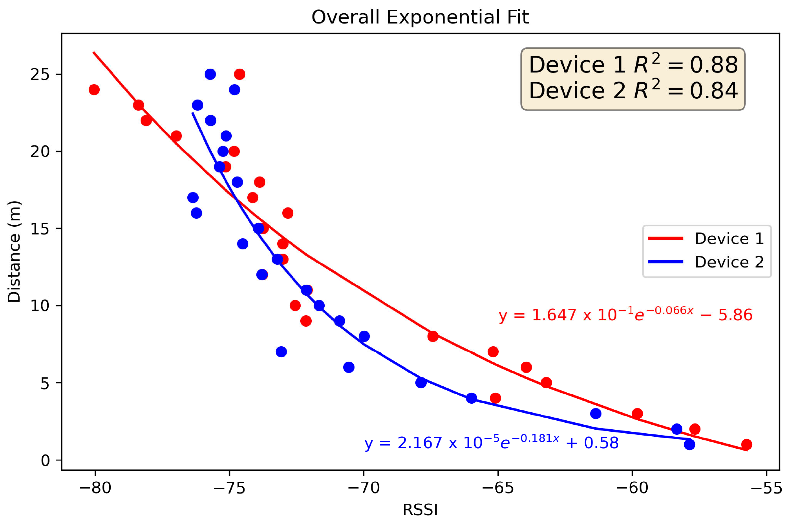
Vector position calculation of the target location is performed by creating a vector with both angle and magnitude parameters between the mobile robot and the target. The direction of the vector can be calculated from the robot orientation and the AoA reading, but the distance between the robot and the target cannot be explicitly obtained from the Bluetooth signal. However, the Bluetooth signal contains an RSSI parameter, which is correlated with the distance between the beacon and the antenna array. An RSSI-to-distance calibration can be performed to estimate the distance based on the RSSI reading, as shown in
Figure 2. Using this calibration, the estimated location of the target (
,
) can be calculated with (1) and (2), where
is the heading of the robot,
is the sensor angle or AoA reading, (
,
) is the current location of the robot, and
d is the estimated distance from the RSSI–distance calibration.
To reduce the impact of sensor noise on the stability of the calculated goal position, at each update event the reported vector goal position is calculated as a time-weighted average of the last 20 calculated vector goal positions. The time-weighting is implemented as an exponential decay function, given by (3), where
is the weight of the
kth position in the vector goal position buffer,
k is the position index in the vector goal position buffer, with
k = 1 corresponding to the most recent calculated goal position, and
is a time-weighting parameter.
The updated vector position
is then calculated using (4) and (5).
5.2. Parallax Position Calulation
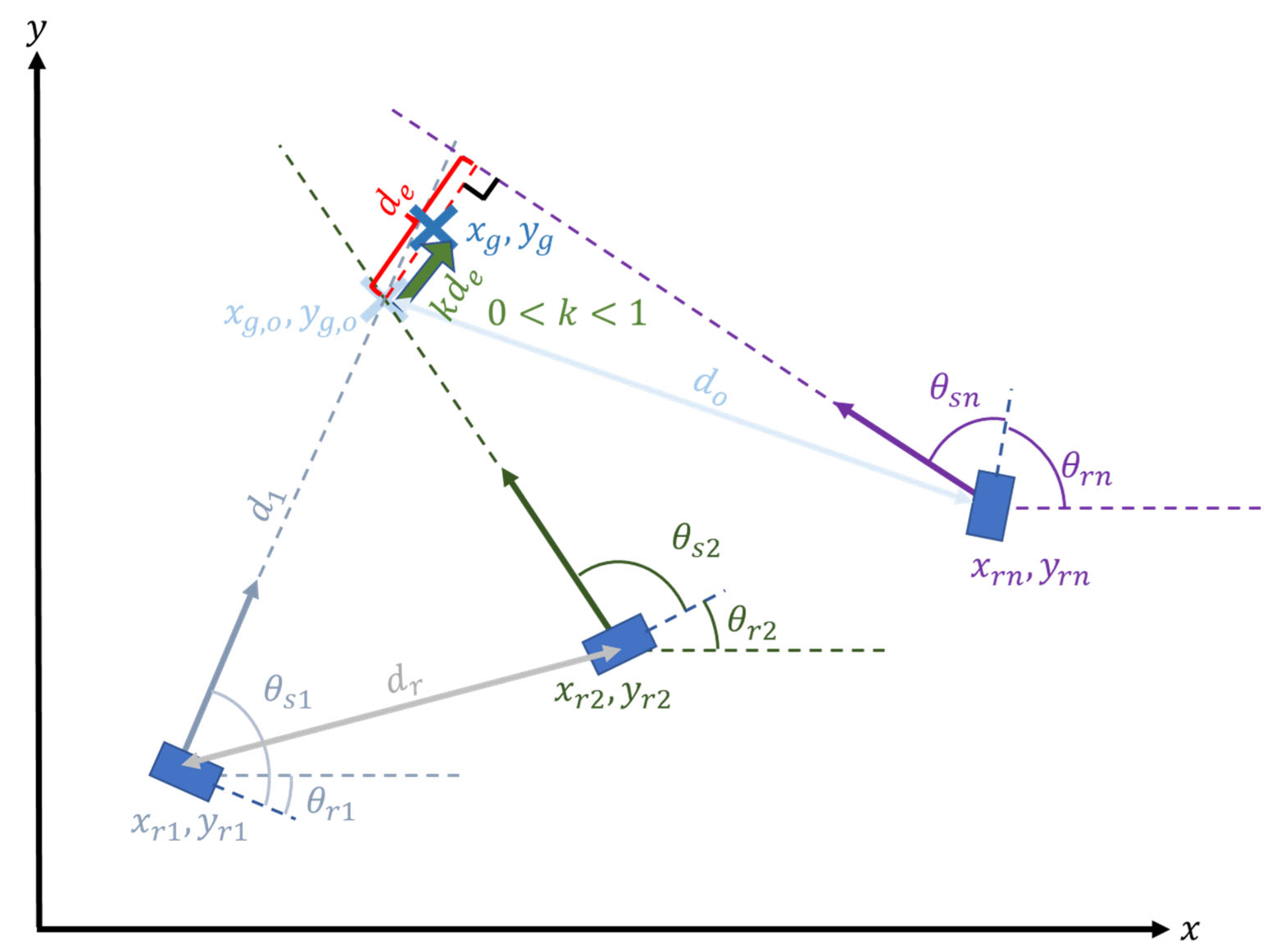
The parallax calculation of the target location utilizes the intersection of vectors obtained from angle readings taken at different locations to determine the target location. This method eliminates the need to know the distance between the robot and the target. However, the goal position updating in this method is more complicated because, in the absence of perfect sensor readings and robot odometry data, there is not a single intersection point for more than two vectors. The initial goal position can be calculated simply using the first two angle readings using (6) and (7),
where
and
Table 1 identifies the variables used in the parallax calculation equations.
Further goal position updates use a Kohonen-learning-inspired updating procedure [
18], which moves the last calculated goal position in the direction of the most recent vector reading according to a parameter,
k (
Figure 3). As more data are acquired, the calculated goal position converges to the actual target position through this continuous updating procedure. The choice of
k is influenced by factors such as sensor noise, updating rate, etc. to achieve stable convergence in a reasonable period of time. It is possible to have
k vary with time, or according to other metrics, but in the examples presented in this paper
k was chosen to be a fixed value. The updating of the goal position is calculated with (10) and (11),
where
and
5.3. Hybrid Controller Implementation
Both vector and parallax position calculations have drawbacks when applied using Bluetooth AoA in this application, preventing robust and accurate convergence to the true target position. Vector position calculation relies heavily on accurate distance measurements. While an approximation of distance between the beacon and the antenna array can be obtained using RSSI-to-distance calibration, there is high variability in RSSI measurements, and the achievable accuracy of the distance estimation is relatively low, resulting in lower accuracy of the reported target position when using these data in the position calculation. Even with filtering of the signal, there is too much uncertainty in the distance estimation achieved using RSSI to attain high localization accuracies using a standalone vector calculation method, as demonstrated by the limited accuracy achieved by other RSSI-based indoor positioning systems. Parallax target position calculation is subject to high error when the angle readings are taken at locations close to each other since the vectors will be near-parallel, creating a large margin of error when calculating the intersection location for slight variations in angle. Due to the fast-updating nature of the controller, angle readings will be taken very close together, resulting in a high probability of early convergence to an inaccurate goal position, especially if the robot starts off facing in the direction of the target.
For the final controller design, a hybrid implementation of both methods of target position calculation was used in order to improve the speed and accuracy of convergence to the target position. In this hybrid implementation, at each time step the updated goal position is calculated using both the vector and parallax calculations, and these are compared as a function of distance to the target for an error metric using (14).
Here, is the parallax goal position, is the vector goal position, and and are the distance between the robot and the goal position for the parallax and vector calculations, respectively. Equation (14) serves as an error-checking method for both goal position estimations by comparing the distance between them. The raw accuracy of the estimated goal positions is correlated with the distance between the robot and the goal position, so the position error metric is normalized by the estimated distance to the target position, calculated as the average distance between each estimated goal position and the robot. The threshold for the error metric was chosen as 0.3 based on the expected noise of the vector position estimations. A lower threshold could result in accurate parallax estimations being flagged as errors due to vector position error noise, while a higher threshold increases the risk of false early convergence of the parallax position estimate due to greater allowable error between the 2 estimations.
The error metric is implemented so that if the error value is less than 0.3, the parallax goal position is reported as the new goal position for that update step. If the error value is greater than 0.3, the vector goal position is checked to see if it is an outlier to the previous 20 vector goal positions using a z-test with a threshold of 1.645, corresponding to a certainty of 90%. If it is not an outlier, then the parallax and vector goal positions are averaged and that location is reported as the new goal location. Additionally, the latest parallax goal position is updated to be equal to this averaged position to reduce the iterations required for convergence. If the latest vector position is an outlier, it is ignored and the parallax goal position is still reported as the new goal position.
The controller continues updating the goal position as described until the robot has arrived at the target. Some potential implementations of the homing controller to achieve a full navigation solution are described in the following paragraphs. Arrival at the target is achieved when the position of the robot is below a specified arrival threshold from the calculated goal position, and the difference between the parallax and vector goal positions is below a specified threshold. The second condition ensures that the robot does not stop before arriving at the target due to early convergence of the parallax goal position calculation.
The goal position updating algorithm described can be applied directly to existing robot control and path-planning algorithms for known environments. In unknown environments, the homing algorithm can be expanded to directly provide goal velocity commands to the robot. The implementation method proposed in this case uses proportional control to determine the linear and angular velocities of the robot as it navigates to the target location. This is carried out by calculating a goal vector between the robot and the target location and using the goal angle and goal distance from this vector to determine the angular and linear velocities, respectively. Additionally, to prevent the robot from moving in a direction away from the target location, the goal linear velocity is modified by the goal angle such that it is set to zero if the absolute value of the goal angle is greater than π/2 radians. Otherwise, it is scaled by the goal angle as given by (15), where
is the goal linear velocity,
is the maximum linear velocity, and
is the goal angle from above.
The homing controller algorithm can further be expanded to incorporate obstacle avoidance in an unknown environment. There are many algorithms for real-time reactive obstacle avoidance, but in this study a simple rule-based obstacle avoidance algorithm was implemented to test homing controller performance when the robot was unable to navigate directly to the target. The obstacle avoidance algorithm used data from a LIDAR sensor and an ultrasonic sensor to detect obstacles. The goal linear and angular velocities were then determined via a set of rules based on the target location and the locations of detected obstacles as the robot moved toward the target.
6. Homing Controller Simulations
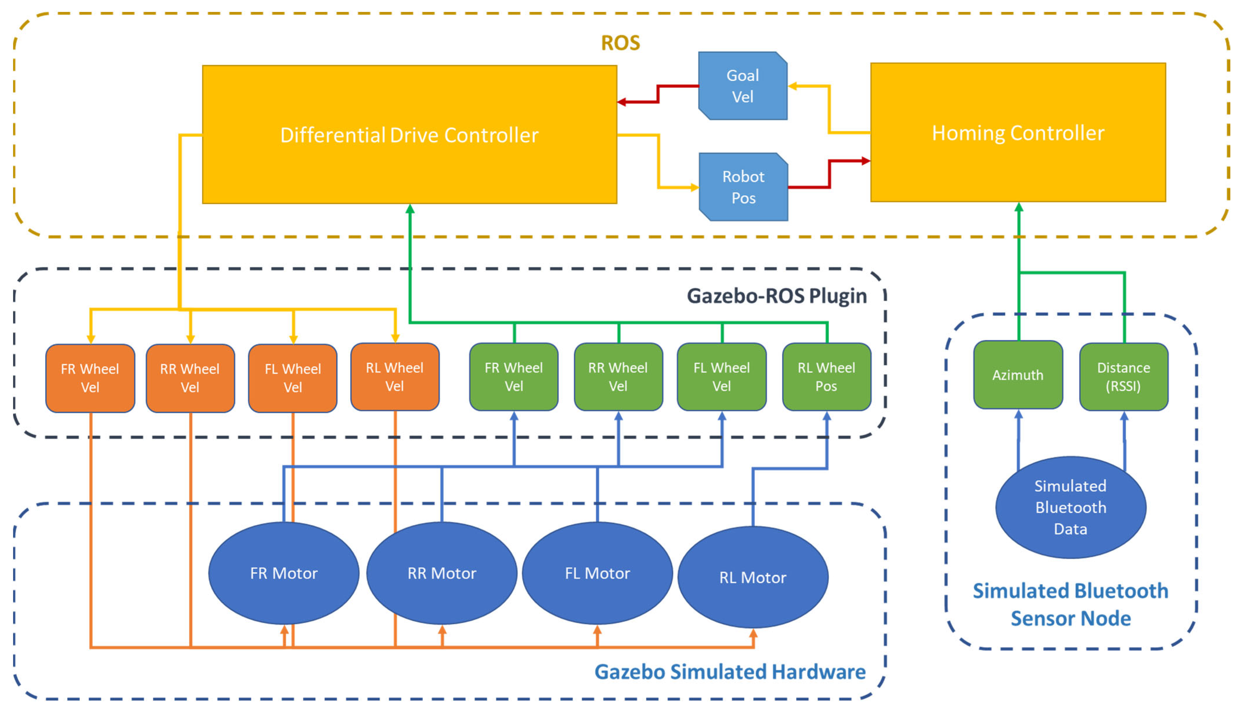
The homing controller algorithm was implemented in ROS and tested via simulations in Gazebo using a 4-wheeled differential drive mobile robot. A custom homing controller plugin was written in ROS using the algorithm described above in combination with the existing differential drive controller in ROS2 control. The output of the homing controller was the goal velocity published to the differential drive controller, which then commanded the wheel motion of the robot. The odometry data of the robot were calculated within the differential drive controller and used by the homing controller. The controller architecture in Gazebo and ROS is shown in
Figure 4. Bluetooth AoA and distance data were simulated with varying levels of sensor noise. For all simulations, the parallax updating parameter,
k, was set to 0.8 and the arrival threshold was set to 0.3 m.
Experiment 1: Homing Controller Algorithm Testing—The performance of the homing controller algorithm was first tested in an obstacle-free environment. The testing area was a −10 m to +10 m square with the robot starting at (0,0) and facing along the +X direction. A total of 40 simulations were performed with 10 randomly determined target locations in each quadrant of the test area for each sensor noise configuration (shown in
Table 2) to evaluate the algorithm sensitivity to sensor noise.
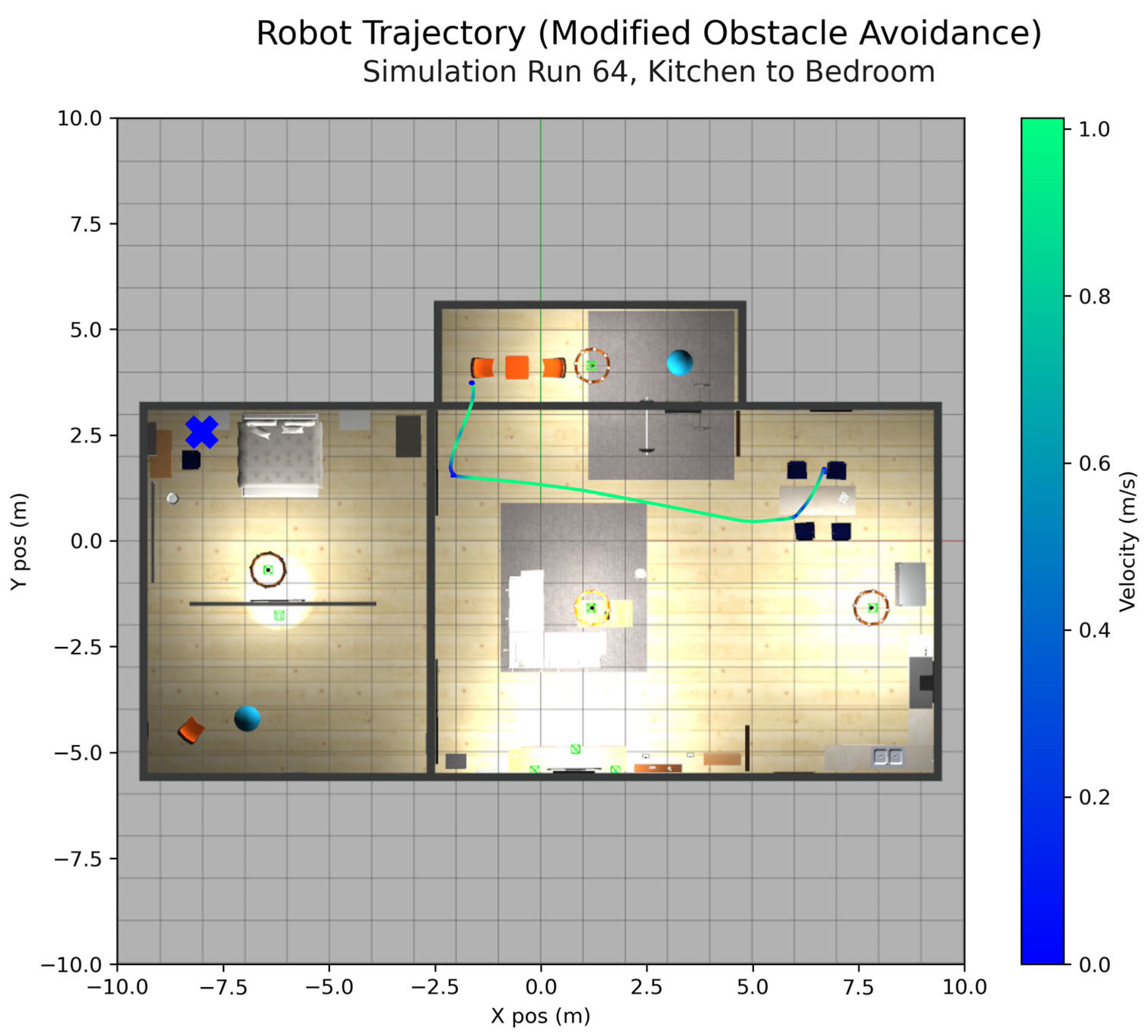
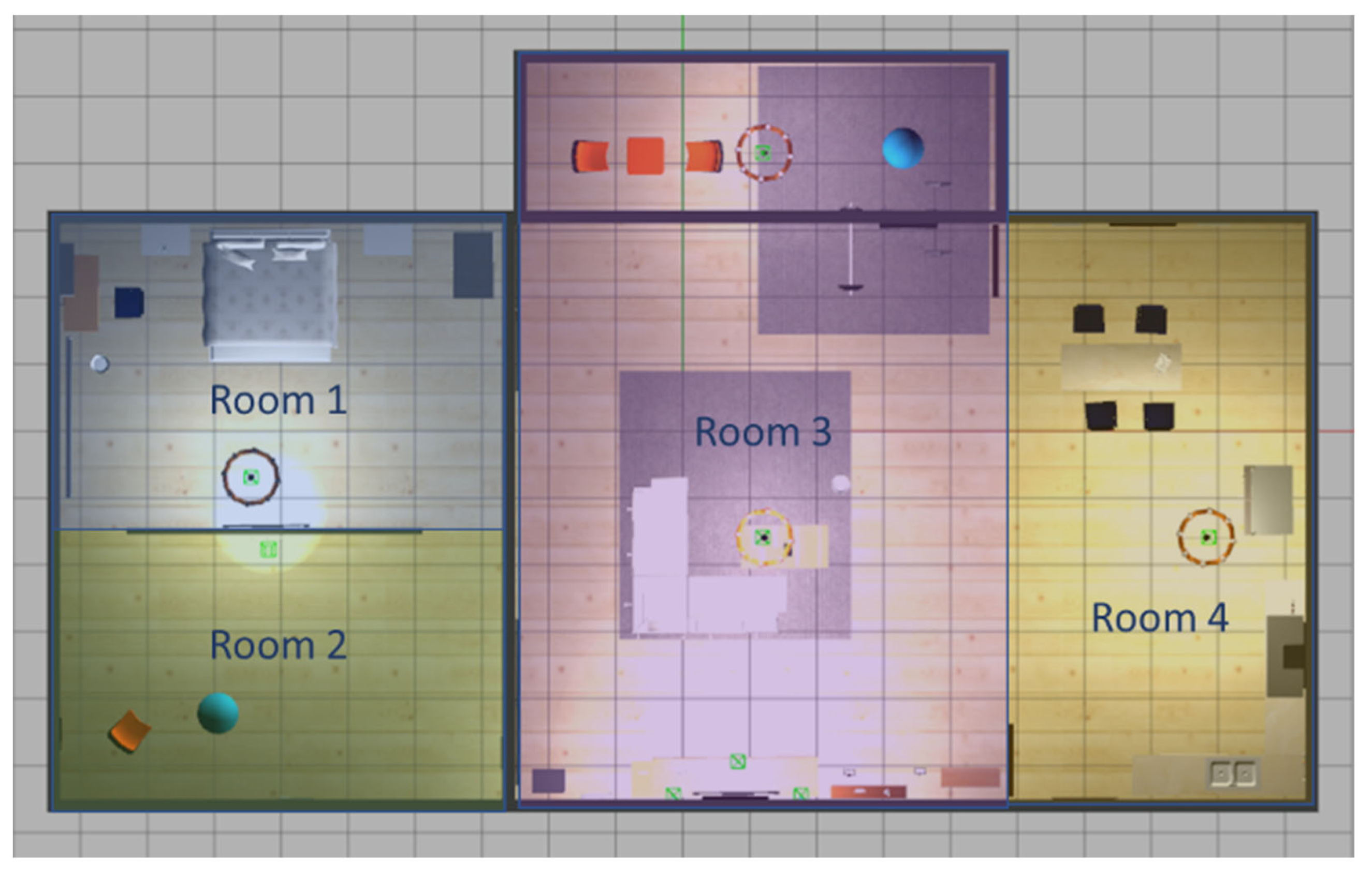
Experiment 2: Homing Controller with Obstacle Avoidance Testing—The homing controller algorithm with obstacle avoidance was tested in a home environment. The AWS Small House World was used as the test environment. The test area was divided into 4 rooms (
Figure 5), and 5 simulations were performed with every combination of start and end room, for a total of 80 simulations. For each simulation, the start location and orientation of the robot and the target location were randomly determined (using a random number generator) within each room. Start and target locations overlapping with objects in the world were not used. All simulations were performed using Bluetooth sensor noise configuration 5. Details on the rule-based obstacle avoidance algorithm implemented for this testing are provided in
Appendix B.
7. Results
7.1. Experiment 1: Homing Controller Algorithm Testing Results
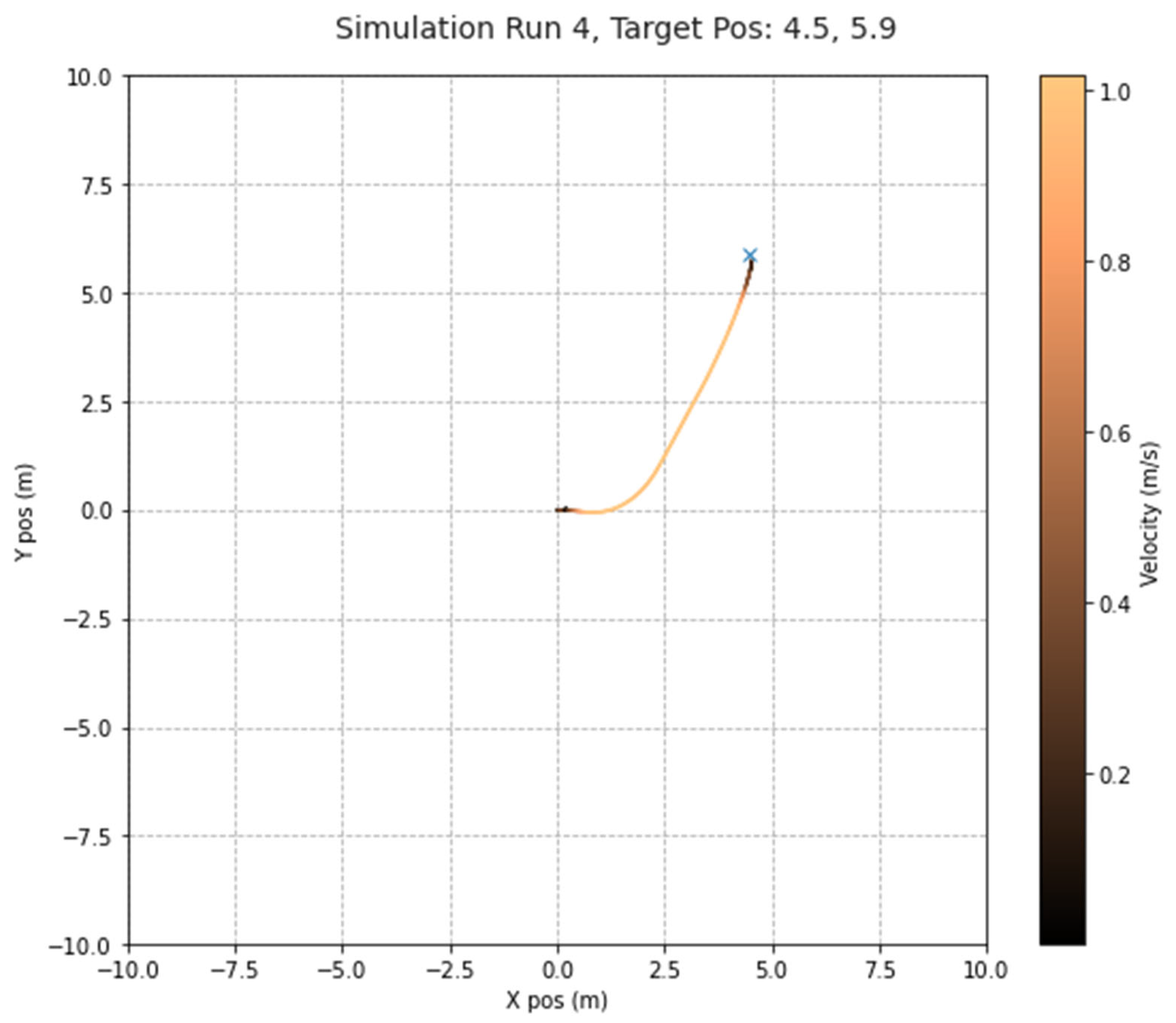
In the obstacle-free simulation testing, the robot had a 100% success rate in navigating to the target location, validating the homing controller algorithm for calculating target position. Additionally, it was found that sensor noise did not have a noticeable impact on controller performance for all tested levels of sensor noise. An example trajectory is given in
Figure 6, and testing performance statistics are given in
Table 3 (see footnotes of
Table 3 for explanation of performance metrics). More detailed results are provided in
Appendix A. In all cases, there was no observed correlation between the location of the target in the test space and the goal position error or final position error. For all sensor noise configurations, there was a clear trend between the net velocity and the distance to the target, with larger distances corresponding to higher net velocities. This makes sense, as the robot would slow down as it approached the target. So, for further targets more time was spent moving close to the maximum velocity. Relatively higher net velocities were also observed for target locations in the first and fourth quadrants of the test area, because in these cases the robot started facing in the general direction of the target and thus did not have to turn around for path correction before proceeding towards the target. Similar results were seen for the path efficiencies, with higher efficiencies observed for farther targets located in the first and fourth quadrants of the test space. This is for similar reasons to the trends in net velocity, as most path inefficiencies occurred at the beginning of the simulations as the robot started moving to determine the general location of the target. Once the general direction of the target was identified, the robot would then turn in that direction before continuing on a more efficient path.
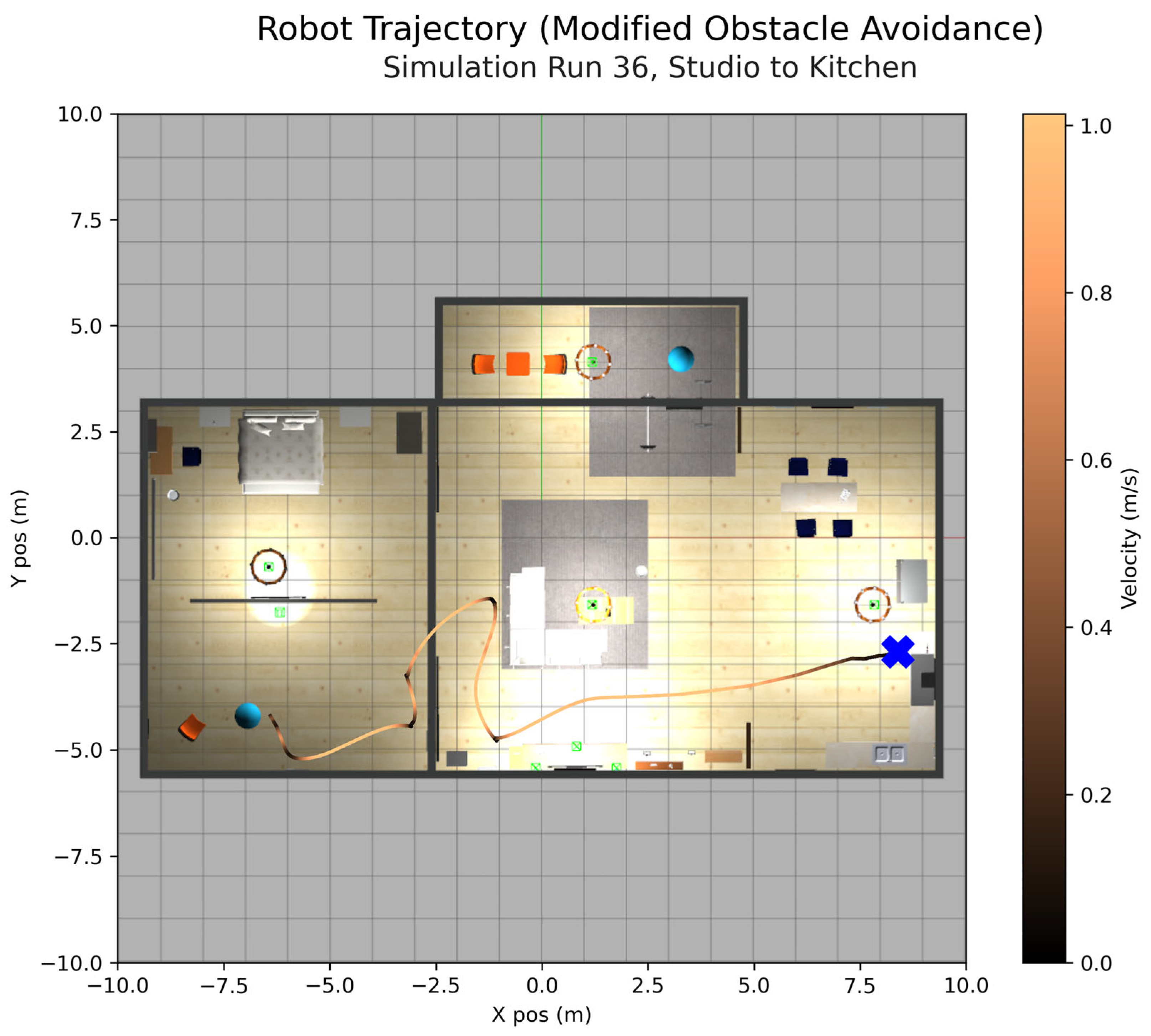
7.2. Experiment 2: Homing Controller with Obstacle Avoidance Testing Results
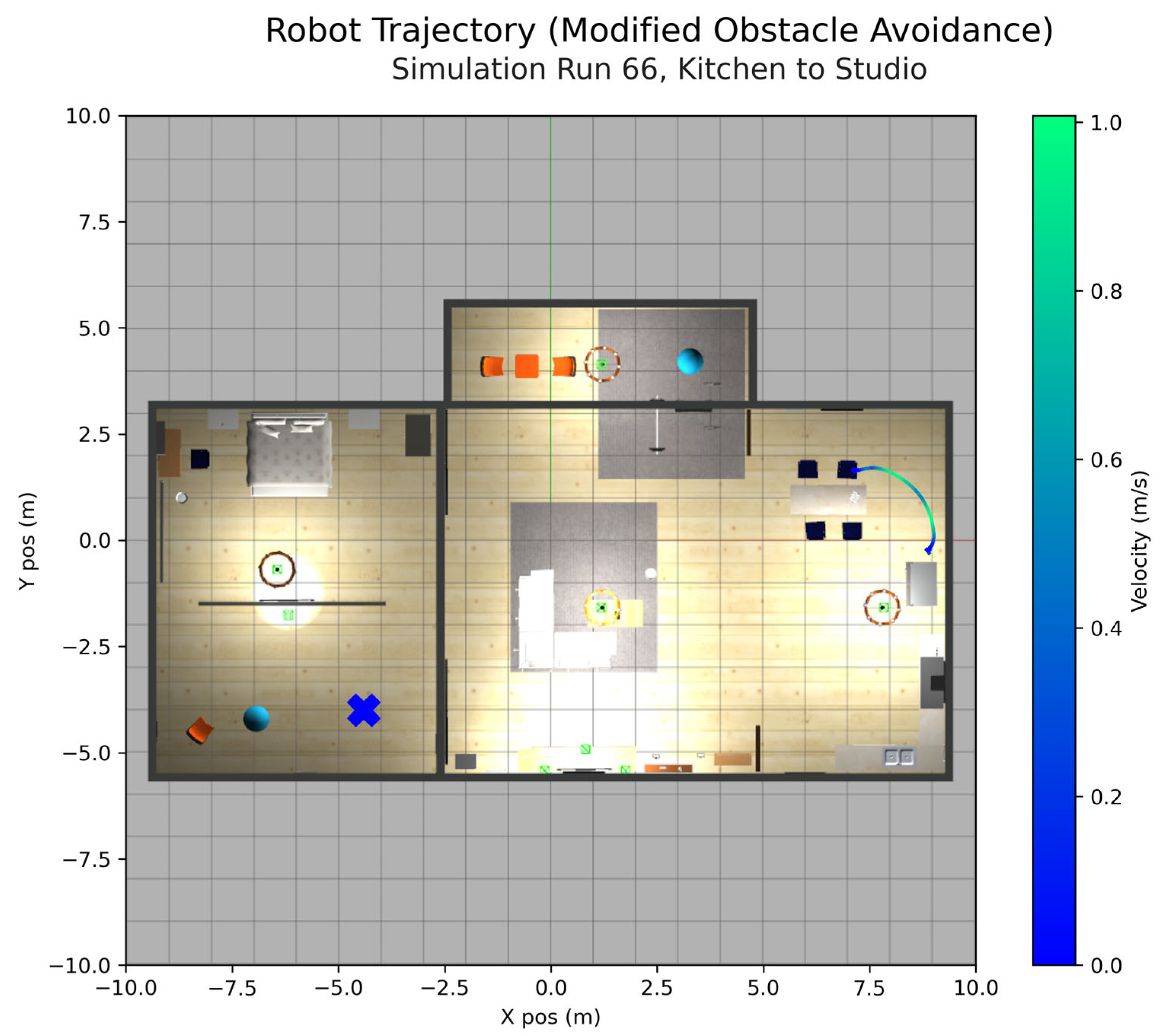
The homing controller with obstacle avoidance had a 96% success rate in navigating to the target. All three failures resulted from the robot hitting an obstacle that was not detected by the sensors and being unable to recover—an expected result for simple rule-based obstacle avoidance such as what was implemented in the controller. Additionally, the mean time to target was much longer and the mean net velocity was much lower than in the obstacle-free scenarios. This is also expected because detours are required for obstacle avoidance, and reactionary rule-based obstacle avoidance generally will not result in the most efficient trajectory to the goal location. Importantly, the mean final position error and goal position error were not significantly higher than in the obstacle-free simulations. This validates the ability of the homing controller algorithm to converge to the correct target position even when the robot is detoured around obstacles, as would be expected in a real-world application scenario. A sample obstacle avoidance simulation trajectory is shown in
Figure 7 and simulation results are given in
Table 4. More detailed results from this testing are provided in
Appendix C.
8. Preliminary Hardware Implementation
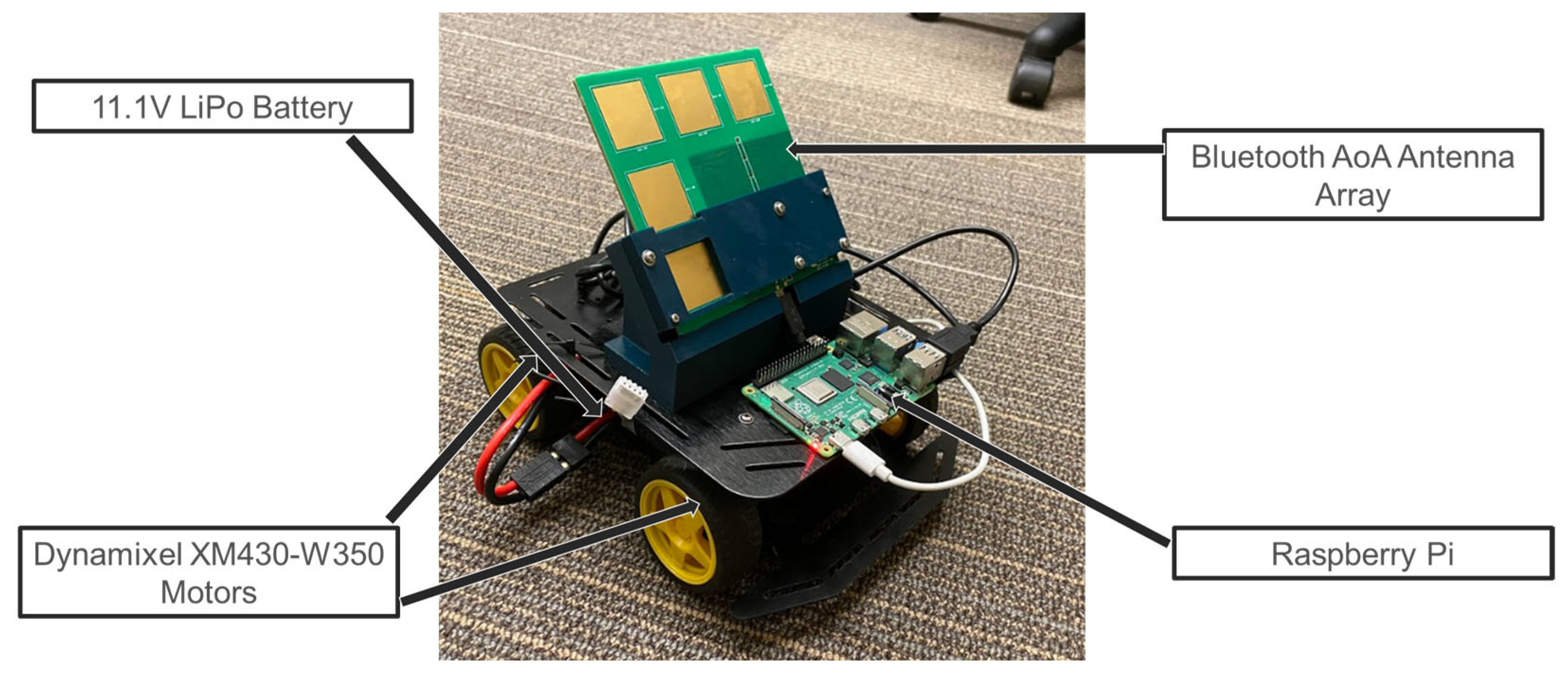
Preliminary testing was conducted on a hardware implementation of the proposed setup using a 4-wheel differential drive robot and the U-Blox XPLR-AOA-1 kit. Testing used ROS on a Raspberry Pi connected serially to the Bluetooth antenna array mounted on the mobile robot.
Figure 8 shows the hardware setup used for testing. This AoA hardware/software implementation only reports angles between ±90°. Due to this constraint, testing was limited to target positions located within this range at the initialization of the controller. Tests were performed using the target location set for the obstacle-free controller simulations, scaled by 0.5 due to space constraints. Preliminary testing yielded a success rate of 85%, with a mean final position error (calculated from successful runs) of 0.27 m. This testing was performed using a baseline antenna array with integrated angle calculation software, so it is likely that results with greater range could be achieved by employing optimization strategies discussed in
Section 3 to improve AoA estimation accuracy.
9. Discussion
Simulation results validated the ability of the Bluetooth AoA-based homing controller algorithm to accurately converge to a desired target position. Additionally, the controller algorithm was successfully implemented as a standalone controller to command goal velocities to navigate the robot to a target location in an unknown environment. This shows the versatility of the algorithm in its ability to produce different outputs (goal position or goal velocity) depending on the implementation for which it is used. While compatibility with path-planning or other existing autonomous navigation algorithms was not tested, it is expected that the controller would be able to converge to an accurate goal position in these implementations as well. Furthermore, the obstacle avoidance simulation testing validated the algorithm in the scenario where the robot is unable to navigate directly to the goal position and must detour along the way. There was no decrease in target position accuracy when the robot was required to take a detour. While the reactionary rule-based obstacle avoidance algorithm implemented in the controller did not perform very efficiently, the main goal of these simulations was to prove compatibility of the algorithm when implemented with other robot control algorithms such as obstacle avoidance. This was confirmed by the continued accuracy of the goal position calculations and indicates that better performance could be achieved by combining the homing controller algorithm with more efficient autonomous navigation algorithms.
The controller algorithm also proved robust to noise in sensor readings, achieving high target position accuracy even in the presence of significant sensor noise. For the presented simulations, the noise level was constant throughout each simulation. It should be noted, however, that in real-world implementations it is expected that sensor noise and accuracy will vary with distance to target and line-of-sight obstructions. While the simulations were performed with high levels of noise to approximate worst-case scenario sensor noise and inaccuracies, future work should include more detailed modeling of variations in sensor readings due to these factors, along with further validation through hardware testing in a range of scenarios, including no line of sight to the target.
The homing controller was implemented such that the goal was to navigate to within 0.3 m of the estimated target location, as described in
Section 5.3. The mean final position errors in all simulations, both obstacle-present and obstacle-free, were below this threshold, validating that in addition to accurately localizing the target, this localization was sufficient to navigate the robot to an acceptable placement with respect to the target. The value of this mean final position error is dependent on the approach distance metric of 0.3 m used for termination of the simulation. A lower final position error could be achieved by reducing this metric, but for most identified potential applications of the proposed homing controller, navigating to within 0.3 m of the target would be sufficient. Once the robot is within this distance, it is likely that additional sensing would be employed to visualize the target and carry out the desired task.
The hardware implementation of AoA technology presents additional challenges, the most significant of which is the current limitation of most algorithms reporting angles only between ±90°. This presents a challenge for the controller if there is not an indication whether or not the angle readings being received are valid and should be used to update the goal position. Preliminary testing validated the algorithm when the target location is within the usable range of the Bluetooth AoA hardware at the activation of the controller, with an 85% success rate, and failures occurred when the starting location was close to the edges of the usable range. There are numerous solutions that could be explored to address the current limitations with AoA hardware, such as signal processing with machine learning and use of other sensors to determine orientation of the antenna array with respect to the target (such as a blocked antenna that only receives signal when facing the target). If it can be determined whether or not the AoA reading is within the good range of the antenna array, the controller algorithm can easily be modified to only update the goal position when the robot is within this range and be commanded to rotate until it is in the range if it is currently outside of the usable range.
10. Conclusions
A Bluetooth AoA homing controller was developed for a mobile robot which enables the robot to navigate to a target object of unknown location by calculating the target location using the AoA and RSSI of the Bluetooth signal. Testing of the controller via simulations showed accurate convergence to the target location, even in the presence of measurement noise, with an MAE of 0.12 m or less, depending on the level of noise. The versatility of the controller was proven through successful navigation to target locations in the presence of obstacles, indicating its compatibility with state-of-the-art autonomous navigation algorithms. It is expected the homing controller could be integrated with most real-time navigation algorithms to create a comprehensive control system. It should be noted that, due to the real-time target localization occurring in the homing controller, this algorithm is not compatible with offline path-planning algorithms. The intended application of this algorithm is for real-time navigation in both known and unknown environments. Directions for future work include investigation of the potential challenges with implementation of the controller framework in hardware, especially regarding the accuracy and range limitations of Bluetooth AoA, and testing of the hardware setup in more complex environments, especially cases where there is not a line of sight to the target so more fluctuations in sensor readings are expected.
Author Contributions
Conceptualization, K.W. and S.S.; methodology, K.W. and S.S.; software, K.W.; validation, K.W.; formal analysis, K.W.; investigation, K.W.; resources, S.S.; data curation, K.W.; writing—original draft preparation, K.W.; writing—review and editing, S.S.; visualization, K.W.; supervision, S.S.; project administration, S.S.; funding acquisition, S.S. All authors have read and agreed to the published version of the manuscript.
Funding
This research was funded by State of Colorado cybersecurity funding, SENATE BILL 18-086. The APC was funded by State of Colorado cybersecurity funding, SENATE BILL 18-086.
Data Availability Statement
Not applicable.
Acknowledgments
The authors acknowledge support for this research from Colorado SB 18-086.
Conflicts of Interest
The authors declare no conflict of interest. The funders had no role in the design of the study; in the collection, analyses, or interpretation of data; in the writing of the manuscript; or in the decision to publish the results.
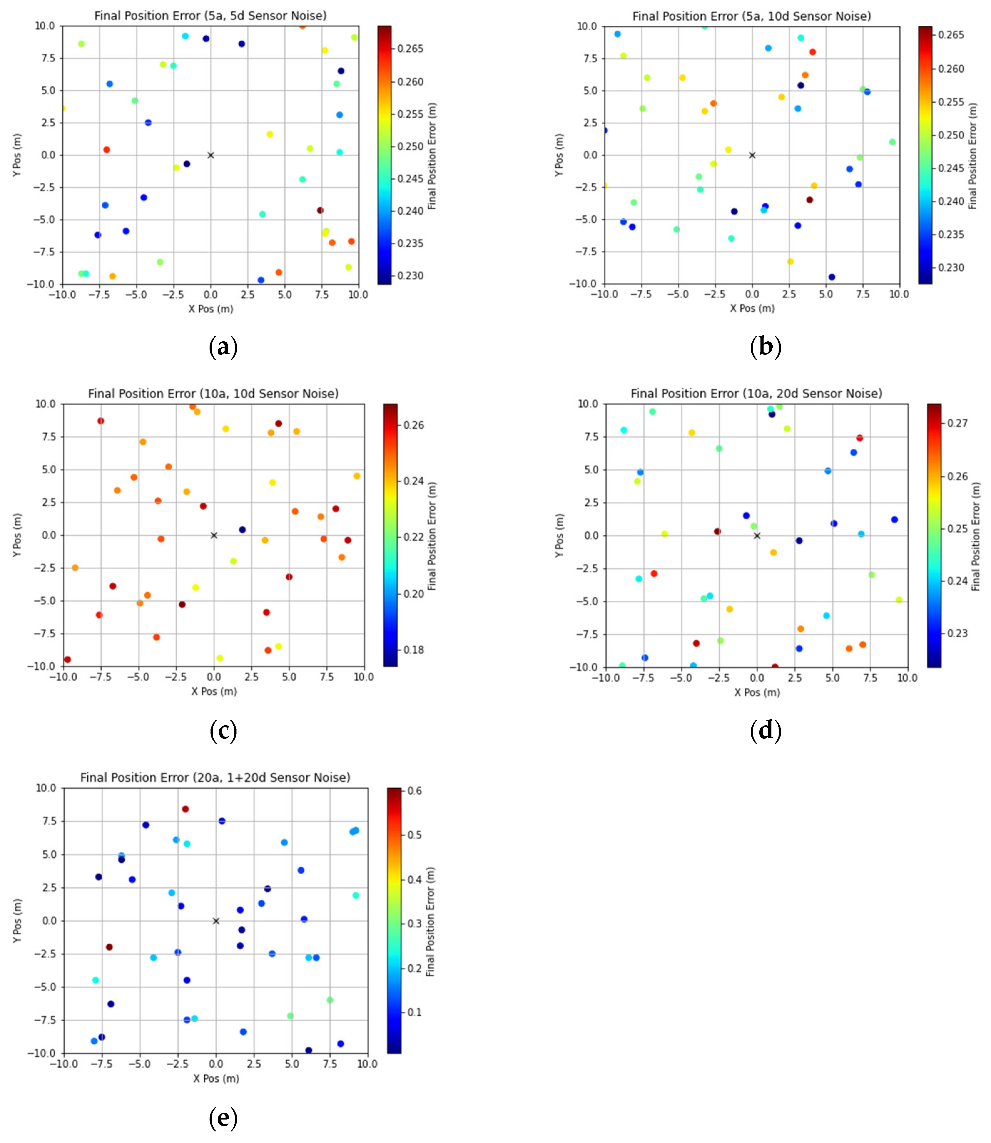
Appendix A. Detailed Homing Controller Algorithm Testing Results
Figure A1.
Final robot position error for each target position simulation by sensor noise configuration as specified in
Table 1: (
a) sensor noise configuration 1, (
b) sensor noise configuration 2, (
c) sensor noise configuration 3, (
d) sensor noise configuration 4, (
e) sensor noise configuration 5.
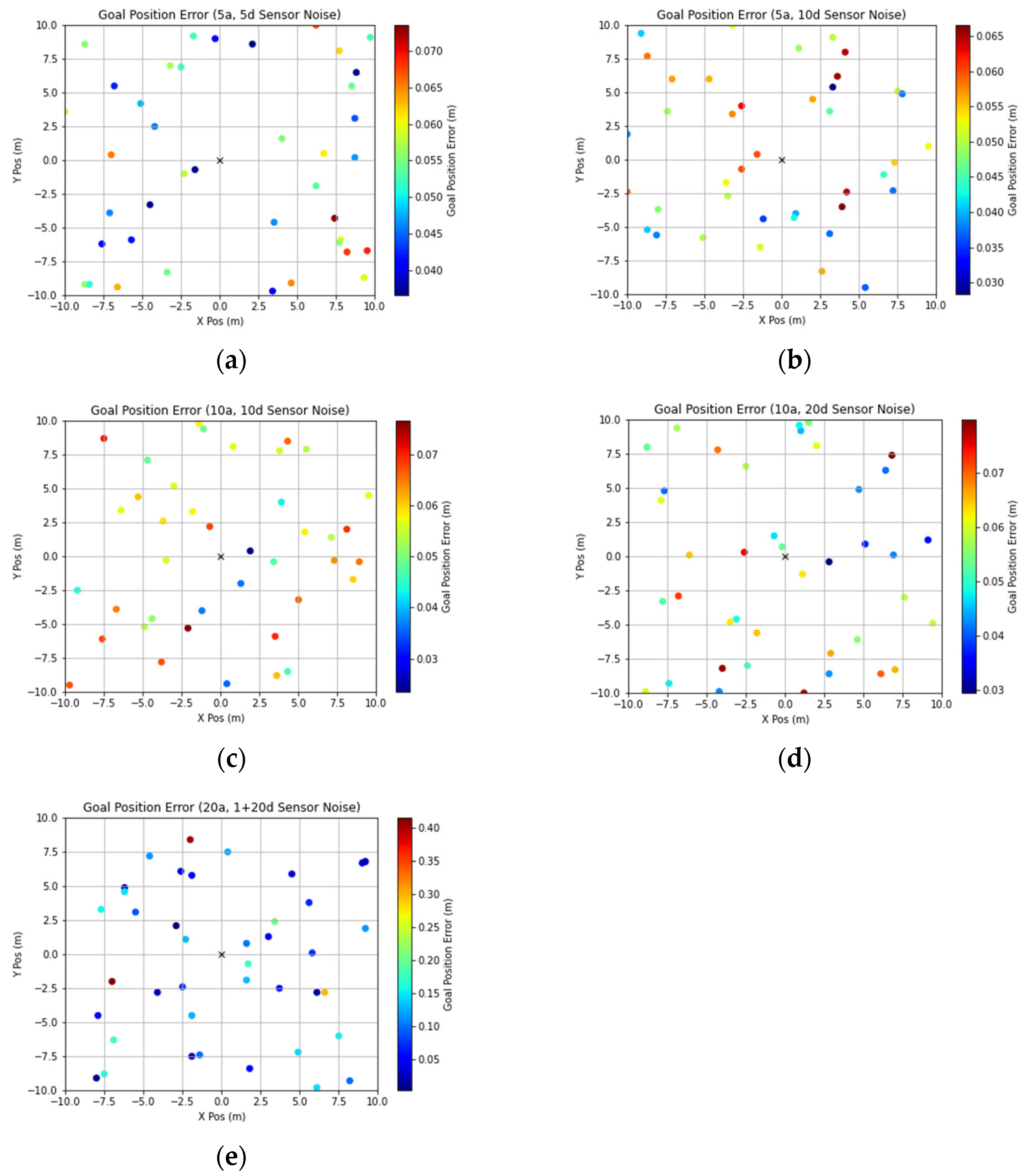
Figure A2.
Goal position error for each target position simulation by sensor noise configuration as specified in
Table 1: (
a) sensor noise configuration 1, (
b) sensor noise configuration 2, (
c) sensor noise configuration 3, (
d) sensor noise configuration 4, (
e) sensor noise configuration 5.
Figure A2.
Goal position error for each target position simulation by sensor noise configuration as specified in
Table 1: (
a) sensor noise configuration 1, (
b) sensor noise configuration 2, (
c) sensor noise configuration 3, (
d) sensor noise configuration 4, (
e) sensor noise configuration 5.
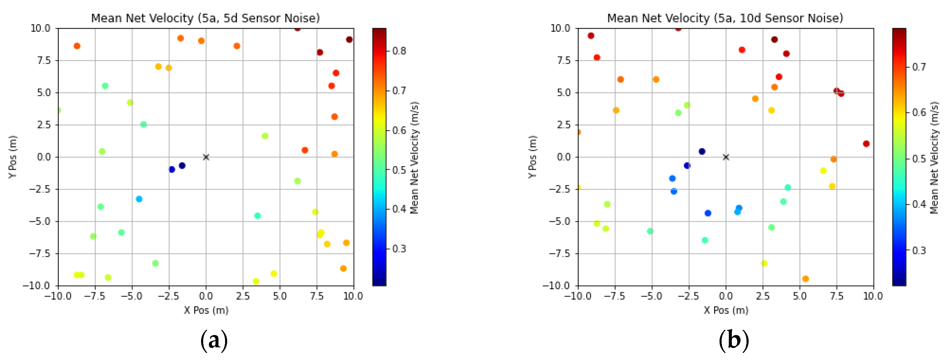
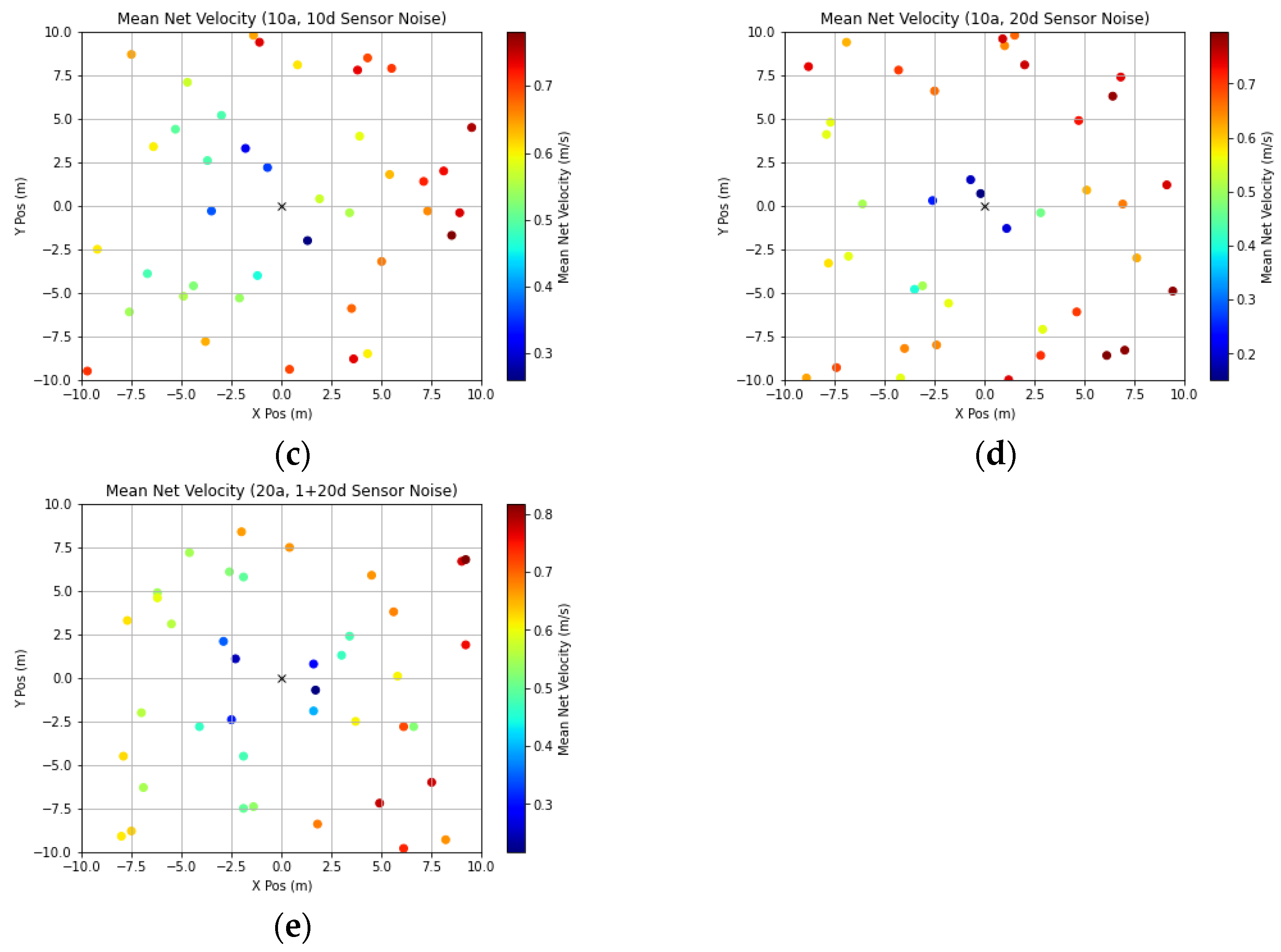
Figure A3.
Mean net velocity for each target position simulation by sensor noise configuration as specified in
Table 1: (
a) sensor noise configuration 1, (
b) sensor noise configuration 2, (
c) sensor noise configuration 3, (
d) sensor noise configuration 4, (
e) sensor noise configuration 5.
Figure A3.
Mean net velocity for each target position simulation by sensor noise configuration as specified in
Table 1: (
a) sensor noise configuration 1, (
b) sensor noise configuration 2, (
c) sensor noise configuration 3, (
d) sensor noise configuration 4, (
e) sensor noise configuration 5.
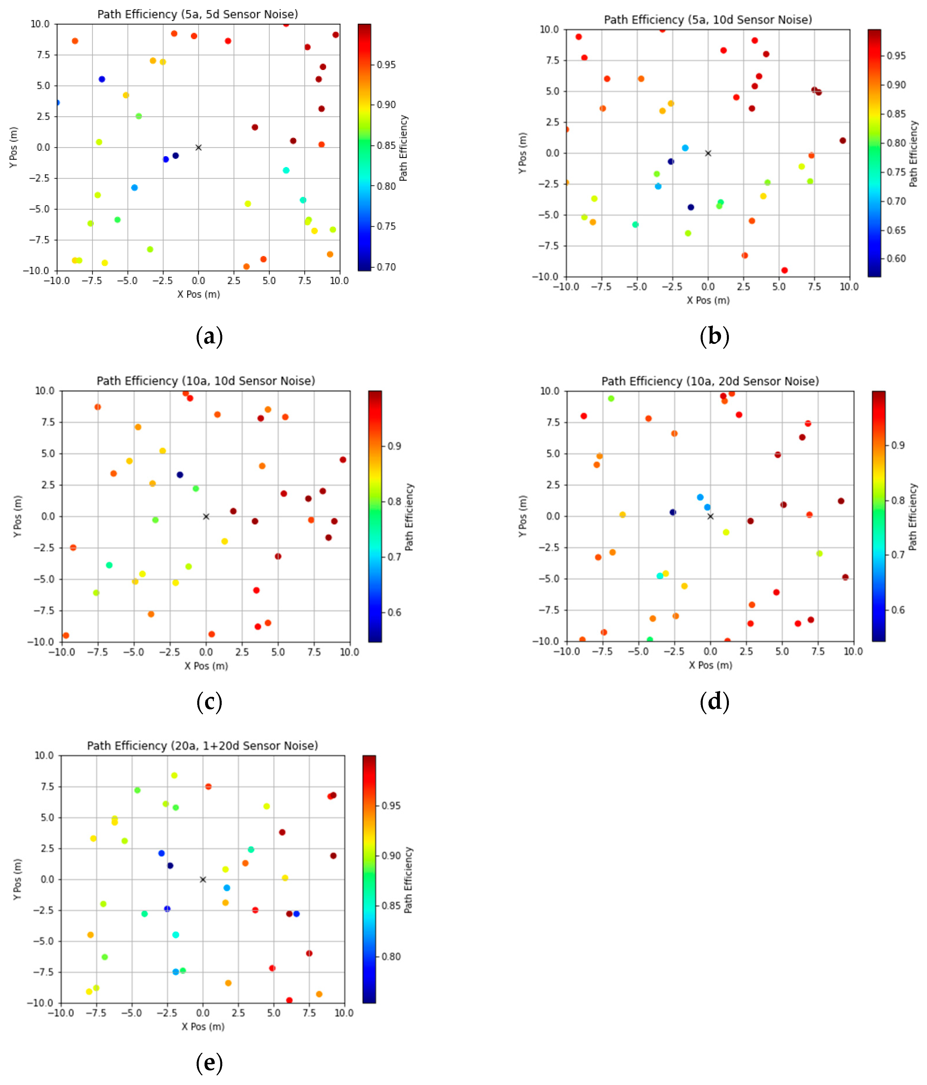
Figure A4.
Path efficiency for each target position simulation by sensor noise configuration as specified in
Table 1: (
a) sensor noise configuration 1, (
b) sensor noise configuration 2, (
c) sensor noise configuration 3, (
d) sensor noise configuration 4, (
e) sensor noise configuration 5.
Figure A4.
Path efficiency for each target position simulation by sensor noise configuration as specified in
Table 1: (
a) sensor noise configuration 1, (
b) sensor noise configuration 2, (
c) sensor noise configuration 3, (
d) sensor noise configuration 4, (
e) sensor noise configuration 5.
Appendix B. Rule-Based Obstacle Avoidance Algorithm
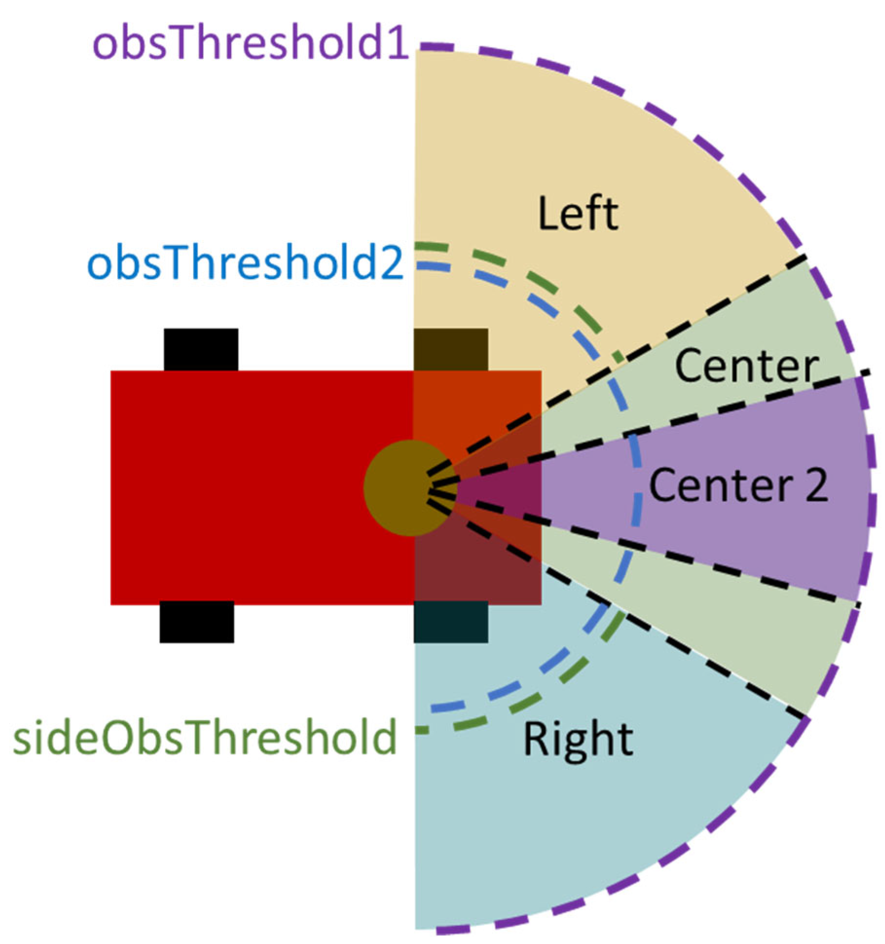
The rule-based obstacle avoidance algorithm implemented in the homing controller testing was based on sensor readings of a LIDAR scanner and an ultrasonic (US) range sensor. The LIDAR scanned over the 180° range in front of the robot, and this range was divided into three equal sections—left, center, and right, as shown in
Figure A5. For each section, the final distance reading was taken to be the shortest distance scanned within the section. Additionally, a ‘center 2′ section was taken as the middle 20% of the scanning region for more precise detection of obstacles directly in front of the robot. Both the ‘center’ and ‘center 2′ LIDAR readings were compared to the US range sensor reading (pointing directly ahead of the robot) and these readings were corrected to the US sensor reading if this value was less than the LIDAR reading to account for obstacles not detected by LIDAR, such as glass.
Figure A5.
LIDAR sensor reading regions for obstacle avoidance algorithm.
Figure A5.
LIDAR sensor reading regions for obstacle avoidance algorithm.
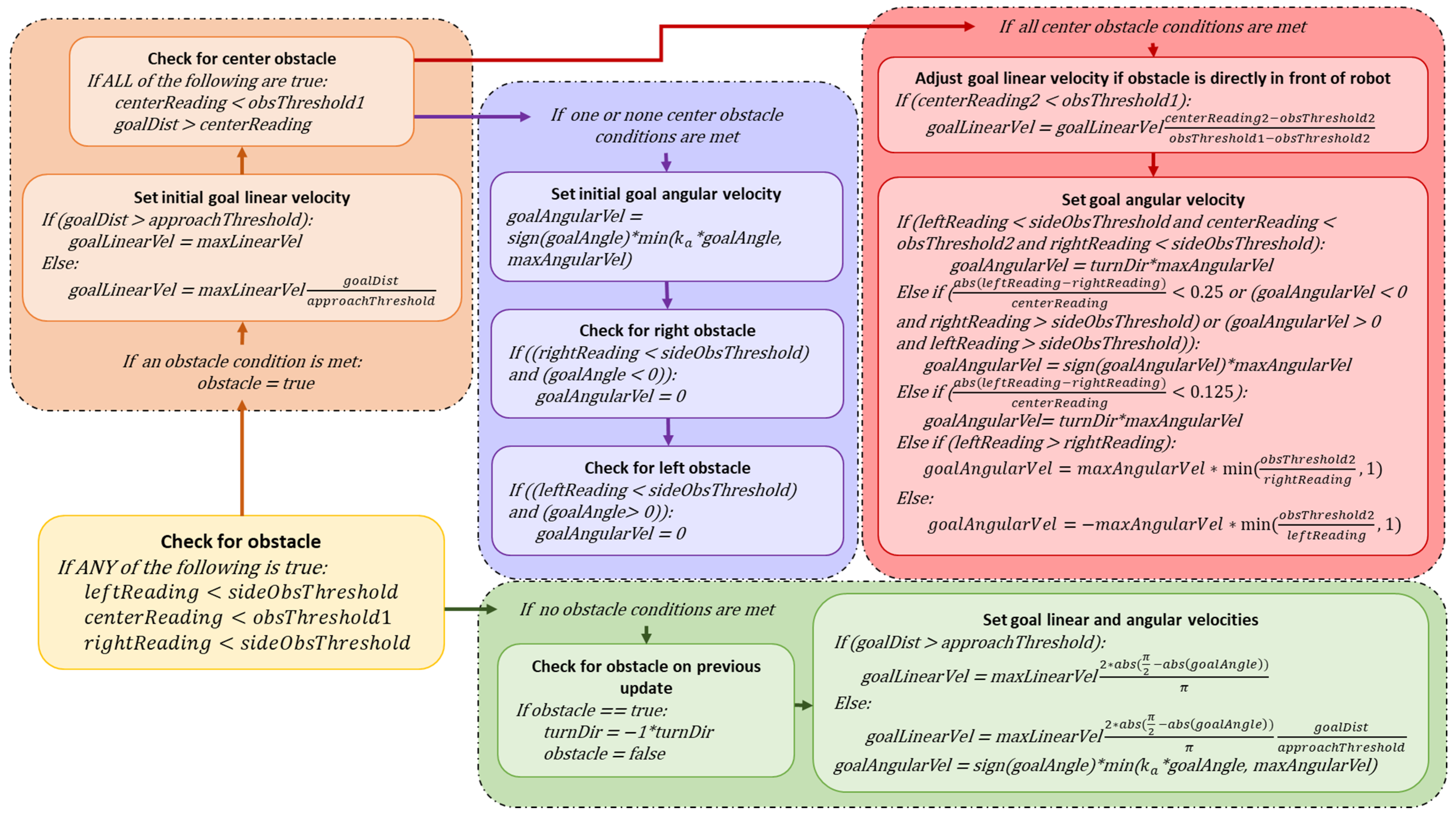
These sensor readings were then used in the obstacle avoidance algorithm shown in
Figure A6 to modify the commanded goal linear and angular velocity if an obstacle were detected. Three different parameters for obstacle avoidance were used, and these values are given in
Table A1.
Table A1.
Obstacle Avoidance Algorithm Parameters.
Table A1.
Obstacle Avoidance Algorithm Parameters.
| Parameter | Value |
|---|
| obsThreshold1 | 1.5 m |
| obsThreshold2 | 0.35 m |
| sideObsThreshold | 0.4 m |
Figure A6.
Flowchart of rule-based obstacle avoidance algorithm used in the homing controller testing with obstacle avoidance.
Figure A6.
Flowchart of rule-based obstacle avoidance algorithm used in the homing controller testing with obstacle avoidance.
Appendix C. Detailed Obstacle Avoidance Homing Controller Testing Results
More detailed results for the obstacle avoidance homing controller testing are provided in this appendix.
Figure A7,
Figure A8,
Figure A9 and
Figure A10 illustrate various performance metrics for every simulation performed in this testing.
Figure A11,
Figure A12 and
Figure A13 show the robot trajectory for the three failed simulations. It can be seen from these figures that all failures occurred due to failure of the obstacle avoidance algorithm, rather than failure to correctly determine the target position.
Figure A7.
Final position error for all obstacle avoidance simulations. Each ‘X’ indicates the actual target position for a simulation, while the corresponding arrow points to the final robot position at the termination of the simulation.
Figure A7.
Final position error for all obstacle avoidance simulations. Each ‘X’ indicates the actual target position for a simulation, while the corresponding arrow points to the final robot position at the termination of the simulation.
Figure A8.
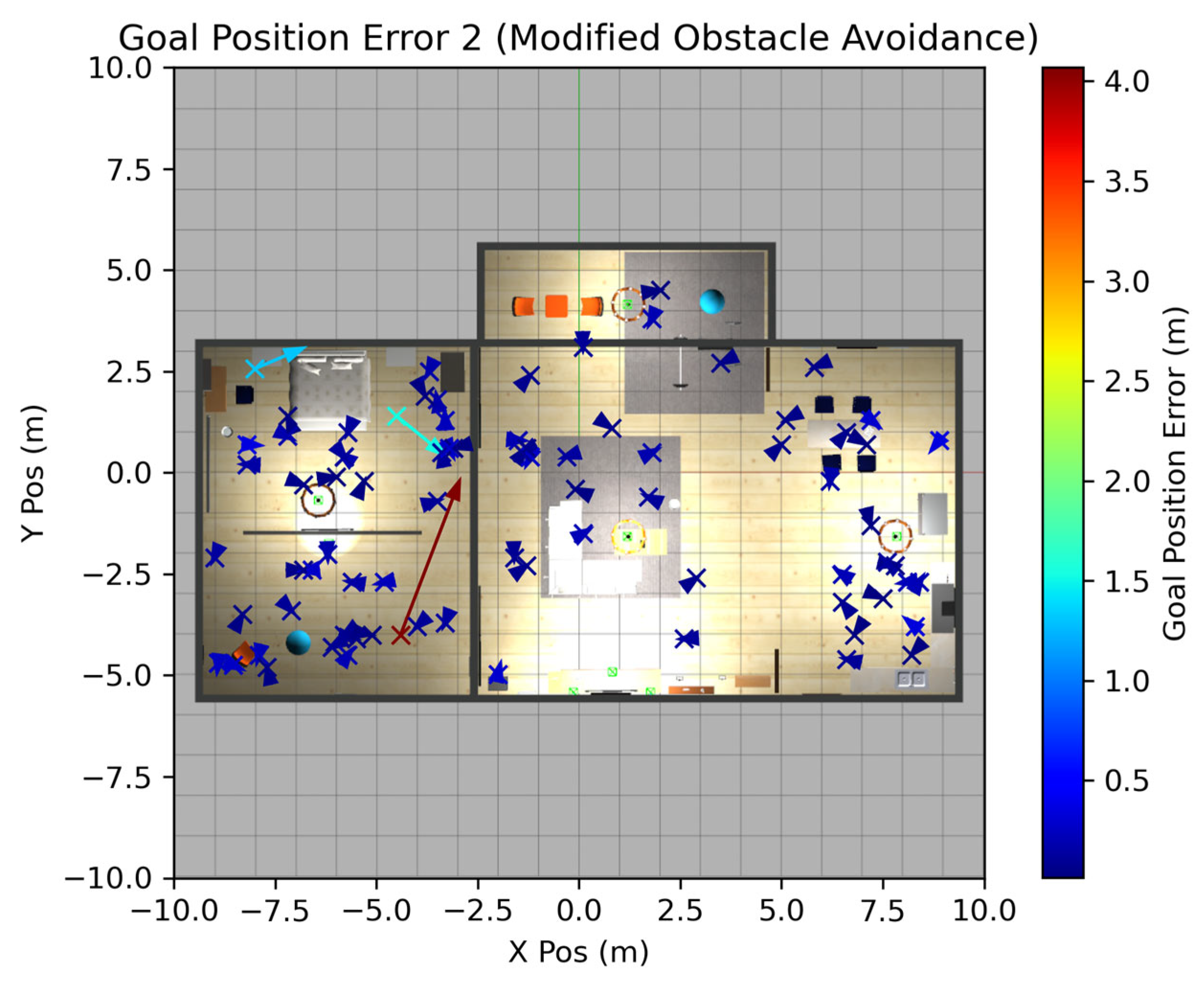
Final goal position error for all obstacle avoidance simulations. Each ‘X’ indicates the actual target position for a simulation, while the corresponding arrow points to the final calculated target position at the termination of the simulation.
Figure A8.
Final goal position error for all obstacle avoidance simulations. Each ‘X’ indicates the actual target position for a simulation, while the corresponding arrow points to the final calculated target position at the termination of the simulation.
Figure A9.
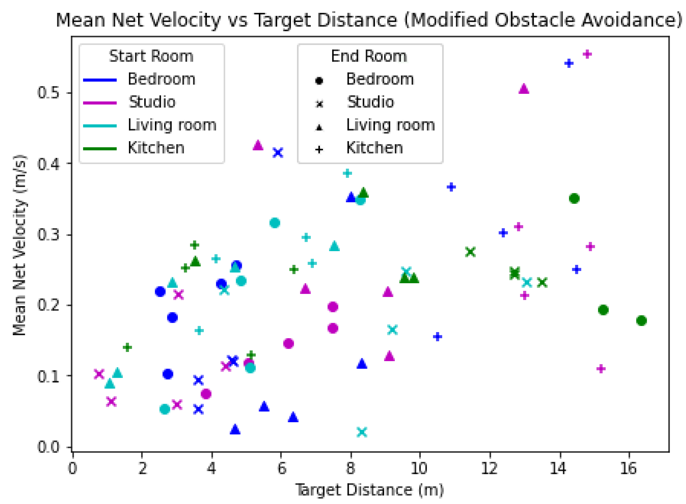
Mean net velocity for all obstacle avoidance simulations plotted versus the distance between the starting position and the actual target position. The start room of the simulation is indicated by the color of the marker, and the end room is indicated by the shape of the marker.
Figure A9.
Mean net velocity for all obstacle avoidance simulations plotted versus the distance between the starting position and the actual target position. The start room of the simulation is indicated by the color of the marker, and the end room is indicated by the shape of the marker.
Figure A10.
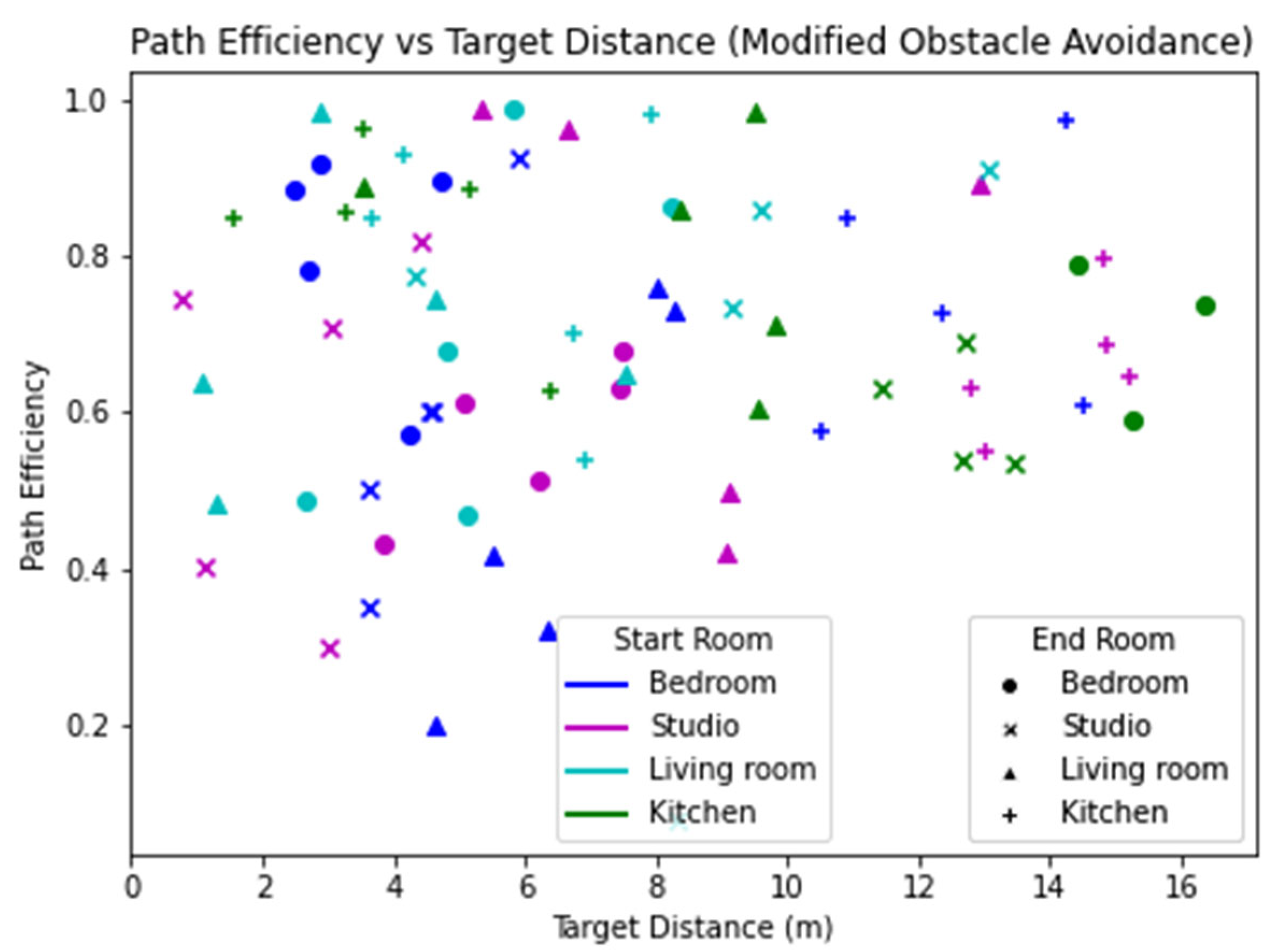
Path efficiency for all obstacle avoidance simulations plotted versus the distance between the starting position and the actual target position. The start room of the simulation is indicated by the color of the marker, and the end room is indicated by the shape of the marker.
Figure A10.
Path efficiency for all obstacle avoidance simulations plotted versus the distance between the starting position and the actual target position. The start room of the simulation is indicated by the color of the marker, and the end room is indicated by the shape of the marker.
Figure A11.
First failed obstacle avoidance simulation. The robot got stuck under the kitchen table and rule-based obstacle avoidance could not get it out of this position. The target position is indicated by the blue ‘X’.
Figure A11.
First failed obstacle avoidance simulation. The robot got stuck under the kitchen table and rule-based obstacle avoidance could not get it out of this position. The target position is indicated by the blue ‘X’.
Figure A12.
Second failed obstacle avoidance simulation. The robot ran into the bottom of a chair that was not detected by the LIDAR and got stuck in this position. The target position is indicated by the blue ‘X’.
Figure A12.
Second failed obstacle avoidance simulation. The robot ran into the bottom of a chair that was not detected by the LIDAR and got stuck in this position. The target position is indicated by the blue ‘X’.
Figure A13.
Third failed obstacle avoidance simulation. The robot ran into a kitchen chair that was not detected by the LIDAR and got stuck. The target position is indicated by the blue ‘X’.
Figure A13.
Third failed obstacle avoidance simulation. The robot ran into a kitchen chair that was not detected by the LIDAR and got stuck. The target position is indicated by the blue ‘X’.
References
- Zhang, D.; Han, J.; Cheng, G.; Yang, M. Weakly supervised object localization and detection: A survey. IEEE Trans. Pattern Anal. Mach. Intell. 2022, 44, 5866–5885. [Google Scholar] [CrossRef] [PubMed]
- Lui, R.; Huskic, G.; Zell, A. Dynamic objects tracking with a mobile robot using passive UHF RFID tags. In Proceedings of the 2014 IEEE/RSJ International Conference on Intelligent Robots and Systems, Chicago, IL, USA, 14–18 September 2014; pp. 4247–4252. [Google Scholar]
- Duan, C.; Rao, X.; Yang, L.; Liu, Y. Fusing RFID and computer vision for fine-grained object tracking. In Proceedings of the IEEE Conference on Computer Communications, Atlanta, GA, USA, 1–4 May 2017. [Google Scholar]
- Yu, X.; Li, Q.; Queralta, J.P.; Heikkonen, J.; Westerlund, T. Applications of UWB networks and positioning to autonomous robots and industrial systems. In Proceedings of the 2021 10th Mediterranean Conference on Embedded Computing, Budva, Bondenegro, 7–10 June 2021. [Google Scholar]
- Ledergerber, A.; Hamer, M.; D’Andrea, R. A robot self-localization system using one-way ultra-wideband communication. In Proceedings of the 2015 IEEE/RSJ International Conference on Intelligent Robots and Systems, Hamburg, Germany, 28 September–2 October 2015; pp. 3131–3137. [Google Scholar]
- Cao, Y.; Yang, C.; Li, R.; Knoll, A.; Beltrame, G. Accurate position tracking with a single UWB anchor. In Proceedings of the 2020 IEEE International Conference on Robotics and Automation, Paris, France, 31 May–2 June 2020; pp. 2344–2350. [Google Scholar]
- Shule, W.; Almansa, C.M.; Queralta, J.P.; Zou, Z.; Westerlund, T. UWB-based localization for multi-UAV systems and collaborative heterogenous multi-robot systems. In Proceedings of the 15th International Conference on Future Networks and Communications, Leuven, Belgium, 9–12 August 2020. [Google Scholar]
- Zhou, S.; Pollard, J.K. Position measurement using Bluetooth. IEEE Trans. Consum. Electron. 2006, 52, 555–558. [Google Scholar] [CrossRef]
- Bandara, U.; Hasegawa, M.; Inoue, M.; Morikawa, H.; Aoyama, T. Design and implementation of a Bluetooth signal strength based location sensing system. In Proceedings of the IEEE Radio and Wireless Conference, Atlanta, GA, USA, 22 September 2004; pp. 319–322. [Google Scholar]
- Wang, Y.; Ye, Q.; Cheng, J.; Wang, L. RSSI-based Bluetooth indoor localization. In Proceedings of the International Conference on Mobile Ad-hoc and Sensor Networks, Shenzhen, China, 16–18 December 2015; pp. 165–171. [Google Scholar]
- Kumar, G.; Gupta, R.; Tank, R. Phase-based angle estimation approach in indoor localization system using Bluetooth low energy. In Proceedings of the 2020 International Conference on Smart Electronics and Communication, Trichy, India, 10–12 September 2020; pp. 904–912. [Google Scholar]
- Hajiakhondi-Meybodi, Z.; Salimibeni, M.; Plantaniotis, K.N.; Mohammadi, A. Bluetooth low energy-based angle of arrival estimation via switch antenna array for indoor localization. In Proceedings of the International Conference on Information Fusion, Rustenburg, South Africa, 6–9 July 2020; pp. 1–6. [Google Scholar]
- Khan, A.; Wang, S.; Zhu, Z. Angle-of-arrival estimation using an adaptive machine learning framework. IEEE Commun. Lett. 2019, 23, 294–297. [Google Scholar] [CrossRef]
- Pau, G.; Arena, F.; Gebremariam, Y.E.; You, I. Bluetooth 5.1: An analysis of direction finding capability for high-precision location services. Sensors 2021, 21, 3589. [Google Scholar] [CrossRef] [PubMed]
- Cominelli, M.; Patras, P.; Gringoli, F. Dead on arrival: An empirical study of the Bluetooth 5.1 positioning system. In Proceedings of the WiNTECH, Los Cabos, Mexico, 25 October 2019; pp. 13–20. [Google Scholar]
- Boccadoro, P.; Colucci, D.; Dentamaro, V.; Notarangelo, L.; Tateo, G. Indoor localization with Bluetooth: A framework for modelling errors in AoA and RSSI. In Proceedings of the IPIN WiP Proceedings, Lloret de Mar, Spain, 29 November–2 December 2021. [Google Scholar]
- Vasilopoulos, V.; Arslan, O.; De, A.; Koditschek, D.E. Sensor-based legged robot homing using range-only target localization. In Proceedings of the International Conference on Robotics and Biomimetics, Macau, China, 5–8 December 2017; pp. 2630–2637. [Google Scholar]
- Haykin, S. Self-Organizing Maps. In Neural Networks and Learning Machines, 3rd ed.; Pearson Ed. Inc.: Upper Saddle River, NJ, USA, 2009; pp. 456–465. [Google Scholar]
| Disclaimer/Publisher’s Note: The statements, opinions and data contained in all publications are solely those of the individual author(s) and contributor(s) and not of MDPI and/or the editor(s). MDPI and/or the editor(s) disclaim responsibility for any injury to people or property resulting from any ideas, methods, instructions or products referred to in the content. |
© 2023 by the authors. Licensee MDPI, Basel, Switzerland. This article is an open access article distributed under the terms and conditions of the Creative Commons Attribution (CC BY) license (https://creativecommons.org/licenses/by/4.0/).


