Coordinating Tethered Autonomous Underwater Vehicles towards Entanglement-Free Navigation

Abstract

This paper proposes an algorithm that provides operational strategies for multiple tethered autonomous underwater vehicle (T-AUV) systems for entanglement-free navigation. T-AUVs can perform underwater tasks under reliable communication and power supply, which is the most substantial benefit of their operation. Thus, if one can overcome the entanglement issues while utilizing multiple tethered vehicles, the potential applications of the system increase including ecosystem exploration, infrastructure inspection, maintenance, search and rescue, underwater construction, and surveillance. In this study, we focus on developing strategies for task allocation, path planning, and scheduling that ensure entanglement-free operations while considering workload balancing among the vehicles. We do not impose restrictions on the size or shape of the vehicles at this stage; our primary focus is on efficient tether management as an initial work on the topic. To achieve entanglement-free navigation, we propose a heuristic based on the primal-dual technique, which enables initial task allocation and path planning while minimizing the maximum travel cost of the vehicles. Although this heuristic often generates sectioned paths due to its workload-balancing nature, we also propose a mixed approach to provide feasible solutions for non-sectioned initial paths. This approach combines entanglement avoidance techniques with time scheduling and sectionalization methods. To evaluate the effectiveness of our algorithm, extensive simulations were conducted with varying problem sizes. The computational results demonstrate the potential of our algorithm to be applied in real-time operations, as it consistently generates reliable solutions within a reasonable time frame.

1. Introduction

Since the first autonomous underwater vehicle (AUV) launched in the 1950s [1], AUVs have expanded human access to the harsh underwater environment, both for scientific research and industrial work. While autonomous navigation in aquatic environments has focused on a single vehicle to overcome the hostile and dynamic nature of the settings, a fleet of AUVs is desirable in many underwater applications, not restricted to search, exploration, monitoring, sampling, and data collection [2,3,4,5]. Proper fleet planning is required for successful mission completion in all these applications based on the AUVs’ structural and functional characteristics. Planning multiple AUVs requires solving three main topics (1) task allocation, (2) path planning, and (3) scheduling, which are correlated with each other and, thus, challenging to solve.

AUVs can be categorized into two classes according to the presence of an umbilical cable. One would be a vehicle with an umbilical cable attached to a control tower called a tethered autonomous underwater vehicle (T-AUV). The second type is one without the cable, called a stand-alone autonomous underwater vehicle (S-AUV). S-AUVs include conventional AUVs, and T-AUVs include ROVs (remotely operated vehicles) and hybrid AUVs. Because the umbilical cable provides a stable power source, real-time communication, and data transfer, T-AUVs benefit from long-duration working-class missions, including underwater ecosystem exploration, infrastructure inspection/maintenance, and search and rescue missions. However, umbilical entanglement can sabotage the mission for single or multi-vehicles or damage the system or other underwater elements. Murphy et al. deployed multiple heterogeneous AUVs at the 2011 Great Eastern Japan Earthquake and reported that the mission was affected by close operations and the fear of tethers tangling or even a collision [6]. Escaping from entanglement is difficult due to the dynamic environment and limited information, especially for human-operated vehicles.

Despite the crucial need for entanglement-free navigation in multiple T-AUV operations, the existing literature on this topic is limited. Specifically, Herts and Lumlsky [7] addressed the entanglement-free simultaneous motion planning problem for a highly specific scenario where each robot moves between a unique pair of start and end nodes. They employed a motion planner to compute a sequential motion for the robots, followed by trajectories that allow for simultaneous movement. While this work represents the only available literature directly related to ours, it falls short in addressing the broader problem we tackle here, which involves task allocation of multiple targets without visiting sequences with multiple target locations and simultaneous entanglement-free path planning.

While many researchers are interested in planning for a fleet of AUVs, relatively limited methods are available [8]. There is increasing interest in advancing techniques for multiple AUVs under various conditions. For instance, in [9], Yao and Qi focused on planning the obstacle avoidance of multiple AUVs in complex ocean environments with the time coordination of simultaneous arrival. Panda et al. [10] proposed a hybrid grey wolf optimization algorithm for collision avoidance with obstacles and other vehicles. Nam [11] proposed data-gathering protocols to support long-duration cooperation by operating long-range AUVs considering energy consumption. A two-stage cooperative path planner was proposed for multiple AUVs operating in a dynamic environment that aims to minimize time consumption with simultaneous arrival while avoiding collisions by Zhuang et al.  [12]. A motion planner that focused on obstacle avoidance for a single AUV was presented by McCammon and Hollinger [13]. Some literature focuses on the motion planning of non-entangling tethers of autonomous vehicles. NEPTUNE [14] solves trajectory planning for multiple tethered robots to reach their individual targets without entanglements, with the algorithm considering the 3D space, and validated with aerial vehicles. Teshnizi and Shell [15] studied a motion planner for a pair of tethered mobile robots. Zhang and Pham [16] proposed a planner that coordinates the planar robot motions to realize a given non-intersecting target cable configuration. Although some state-of-art techniques have considered heterogeneous fleets of AUVs, entanglement-free constraints have not been considered in the planning. We aim to fill this gap and build a foundation by providing good approximate solutions with lighter computational loads.

In our preliminary work, the task allocation and path planning problems for multiple structurally heterogeneous autonomous ground vehicles were studied to minimize the last job completion time [17,18]. While working on these problems, we observed that the heuristics often produce sectioned paths due to the nature of workload balancing. The sectioned paths used in this paper represent each path in a 3D space that does not intersect with other paths. Based on this observation, we propose an extended algorithm applicable to multiple AUVs by introducing an extra dimension and additional steps to ensure no entanglement happens during operations. This novel approach to the problem is rarely studied but is essential in operations for multiple T-AUVs. The proposed approach has been tested extensively in simulation environments. While this paper does not include field testing, it is worth noting that the Intelligent Robotics and System Optimization Laboratory (IRoSOL) at Michigan Tech possesses multiple BlueROV2 vehicles, measuring 457 mm in length, 338 mm in width, 254 mm in height, and weighing 10 kg in air. These resources offer promising opportunities for conducting field tests in the future.

The remainder of this paper is structured as follows: In Section 2, we specify the problem and present the formulations. Section 3 presents the heuristic approach to the problem. The computational results are shown in Section 4, and finally, we conclude the paper in Section 5.

2. Problem Description and Formulation

In this work, our objective is to address the problem of coordinating T-AUVs in navigating a set of targets. We aim to find paths for each vehicle that satisfy the following criteria: (1) All targets are visited by at least one AUV; (2) each path adheres to the motion constraints specific to the corresponding vehicle; (3) the tethers of the vehicles are kept at a safe distance from each other to avoid entanglement; and (4) the maximum travel cost among the vehicles is minimized. The initial setup assumes that the AUVs start at distinctive depots on the surface and return to these depots once they have visited all their assigned targets. To simplify the problem, several assumptions are made. First, we assume symmetrical travel costs that adhere to the triangle inequalities. The vehicles are considered holonomic and homogeneous, with the travel cost determined as the travel time between targets using the average running velocity of the vehicles. Additionally, we assume that the cable connecting the vehicle and the depot is a straight line managed by a tether control system without requiring extensive cable release. While these assumptions enable us to present an initial exploration of the problem, our future work aims to incorporate dynamic features of the tether shape for a more comprehensive solution.

If we relax constraint (3) stated above, the problem can be formulated into a min–max multiple depot heterogeneous Traveling Salesman Problem (TSP), first introduced in [17]. We use the dual formulation of the linear program relaxation of the problem to generate a minimum spanning forest, which becomes the initial task assignment. In the formulation, the following definitions are used for the variables.

Variable Definitions:

T	the set of targets
m	the number of vehicles in the cohort
$d_k$	the depot of the k-th vehicle
$V_k$	the set of nodes that contains targets and the depot for k-th vehicle
$E_k$	the set of edges between the nodes in $V_k$
${\delta }_k\left(S\right)$	the subset of the edges of $E_k$ with one end in S, and the other end in $V_k\setminus S$

$$\begin{array}{cc}\hfill C_{dual}& =max2\sum _{S\subseteq T}{Y}_1\left(S\right)\hfill \end{array}$$

(1)

$$\begin{array}{cc}\hfill \sum _{S:e\in {\delta }_k\left(S\right)}{Y}_k\left(S\right)& \le cos{t}_{ij}^k{W}_k\forall i,j\in V_k,k=1,\cdots ,m,\hfill \end{array}$$

(2)

$$\begin{array}{cc}\hfill \sum _{S\subseteq U}{Y}_k\left(S\right)& \le \sum _{S\subseteq U}{Y}_{k+1}\left(S\right)\forall U\subseteq T,k=1,\cdots ,m-1,\hfill \end{array}$$

(3)

$$\begin{array}{cc}\hfill \sum _{k=1,\cdots ,m}{W}_k& \le 1\hfill \end{array}$$

(4)

$$\begin{array}{cc}\hfill Y_k\left(S\right)& \ge 0\forall S\subseteq T,k=1,\cdots ,m,\hfill \end{array}$$

(5)

$$\begin{array}{cc}\hfill W_k& \ge 0k=1,\cdots ,m.\hfill \end{array}$$

(6)

In this formulation, $Y_k\left(S\right)$ can be interpreted as the prices that all targets in the set S are willing to pay to be connected to $d_k$, while $W_k$ are treated as the gains for giving priority to the vehicles. Once the initial task allocation is derived, we solve the entanglement problem as the next step. The details will be explained in the following section.

3. A Heuristic for Entanglement-Free Coordination of Multiple Tethered AUVs

The proposed heuristic for coordinating multiple T-AUVs consists of two main steps: (1) Producing an initial task allocation and routes by relaxing the entanglement constraint; and (2) detecting and resolving the possible tether entanglements. We solved the initial task allocation and routing problem with a primal-dual heuristic while following the main structure of the algorithm presented in [17] but with some revisions. The heuristic is developed based on the dual formulation (1)–(6) while iteratively changing the $W_k$ values to improve the workload distribution. With fixed $W_k$ values, the heuristic runs Algorithm 1 to find a task assignment and routes. To present the algorithm easier to understand, we have divided the steps into three and presented them in Algorithms 2–4. Starting from all zero dual variables, in each iteration, the dual variables $Y_k\left(S\right)$ that tightens one of the dual constraints, (2) or (3), is increased. If (2) becomes tight, a corresponding edge is added to the forest, and if (3) becomes tight, the corresponding set is marked and potentially connected to another depot with lower cost. The main loop terminates once every target is connected to at least one depot. The pruning steps guarantee the assignment of tasks to only one vehicle while trying to improve the workload balancing. Based on the results from fixed $W_k$ values, the algorithm adjusts the $W_k$ values to decrease the maximum travel cost while not violating the monotonic cost increase condition, i.e., $W_{1}cos{t}_{ij}^1\le W_{2}cos{t}_{ij}^2\le \cdots \le W_{m}cos{t}_{ij}^m$; subsequently, the best trial is chosen. When m vehicles and n targets are given, the following notations are utilized to present the algorithms.

Algorithm notations:

$R_k$	The $k^{th}$ vehicle
$F_k$	A set of edges in the graph of $R_k$
${\mathcal{C}}_k$	A collection of vertex sets in the graph of $R_k$
$Y_k\left(S\right)$	The dual variable of set S for $R_k$
$d_k$	The depot for $R_k$
$dua{l}_k\left(v\right)$	The sum of dual variables for all sets that contain vertex v
$boun{d}_k\left(S\right)$	The sum of $Y_{k+1}\left(S\right)$
$Childre{n}_k\left(S\right)$	The vertex sets of S that exist in the graph for $R_{k+1},\cdots ,R_m$
$activ{e}_k\left(S\right)$	The variable that represents whether $Y_k\left(S\right)$ can be increased
	$activ{e}_k\left(S\right)=\left\{\begin{array}{c}1\mathrm{if}\mathrm{set}S\mathrm{can}\mathrm{increase}\mathrm{its}\mathrm{dual}\mathrm{variable}\hfill \\ 0\mathrm{otherwise}\hfill \end{array}\right.$
$Cost=\{C{o}_1,\cdots ,C{o}_m\}$	A set of edge costs
$Tour=\{T{r}_1,\cdots ,T{r}_m\}$	A set of routes
$W=\{W_1,\cdots ,W_m\}$	A set of all $W_k$
$S_k$	The location of $R_k$
$T_k$	The heading target location from $S_k$
$L_k^t$	The estimated location of $R_k$ between $S_k$ and $T_k$
	at time t, where t is a parameter
$\overrightarrow{C{V}_k^t}$	The cable vector connecting $L_k^t$ and $d_k$
$C{P}_k$	The cable plane that contains $d_k$ and two targets assigned to $R_k$ in sequence
$\overrightarrow{C{S}_{ij}}$	The vector connecting $d_i,d_j$
$R_{yield}$	The vehicle which is made to yield
$R_{pass}$	The vehicle that passes
v	The average moving velocity of the AUVs
$D_z$	$z^{th}$ departure among chronologically arranged $n+m$ scheduled departures of all vehicles

Algorithm 1 Tour=GetPartition($Cost,W$)

1: $W_k=1/k$ for $k=1,\cdots ,m$; 2: $[F_k,{\mathcal{C}}_k,activ{e}_k,Childre{n}_k]=Initialization(m,V_k,d_k)$ 3: $F_k=Mainloop(F_k,{\mathcal{C}}_k,activ{e}_k,Childre{n}_k,Cost,W)$ 4: $Tour=Pruning(F_k,Cost,W)$ 5: Adjust $W_k$ that satisfies the monotonic cost increase condition. 6: Repeat 2–4 until there is no improvement in the cost. 7: Choose the best $Tour$ that produces the minimum $max\left(TourCost\right)$

Algorithm 2 $[F_k,{\mathcal{C}}_k,activ{e}_k,Childre{n}_k]=Initialization(m,V_k,d_k)$

1: $F_k\leftarrow \varnothing$, ${\mathcal{C}}_k\leftarrow \{\left\{v\right\}:vs.\in V_k\}$, for $k=1,\cdots ,m$ 2: All the vertices are unmarked. 3: All the dual variables are set to zero. 4: $activ{e}_k\left(\left\{v\right\}\right)\leftarrow 1$, $\forall vs.\in V_k$, for $k=1,\cdots ,m$ 5: $activ{e}_k\left(\left\{d_k\right\}\right)\leftarrow 0$, for $k=1,\cdots ,m$ 6: $Childre{n}_k\left(\left\{v\right\}\right)\leftarrow \left\{v\right\}$, $\forall k=1,\cdots ,m-1$;

Algorithm 3 $F_k=Mainloop(F_k,{\mathcal{C}}_k,activ{e}_k,Childre{n}_k,Cost,W)$

1: while there exists any active component in ${\mathcal{C}}_1$ do 2:    for $k=1,\cdots ,m$ do 3:      Find an edge $e_k=(i,j)\in E_k$ with $i\in C_i,j\in C_j$ where $C_i,C_j\in {\mathcal{C}}_k,C_i\ne C_j$ that minimizes 4:      ${\epsilon }_k^1=\frac{\{W_{k}cos{t}_{ij}^k-dua{l}_k\left(i\right)-dua{l}_k\left(j\right)\}}{activ{e}_k\left(C_i\right)+activ{e}_k\left(C_j\right)}$. 5:    end for 6:    for $k=1,\cdots ,m-1$ do 7:      Let $\Re :=\{R:activ{e}_k\left(R\right)=1,Children\left(R\right)=\varnothing ,R\in {\mathcal{C}}_k\}$. Find $\overline{R}\in \Re$ that minimizes ${\epsilon }_k^2=boun{d}_k\left(\overline{C}\right)-Y_k\left(\overline{R}\right)$ 8:    end for 9:    ${\epsilon }_{min}=min({\epsilon }_1^1,\cdots ,{\epsilon }_m^1,{\epsilon }_1^2,{\epsilon }_{m-1}^2)$ 10:    for $k=1,\cdots ,m$ do 11:      for $C\in {\mathcal{C}}_k$ do 12:         $Y_k\left(C\right)\leftarrow Y_k\left(C\right)+{\epsilon }_{min}activ{e}_k\left(C\right)$ 13:         $dua{l}_k\left(v\right)\leftarrow dua{l}_k\left(v\right)+{\epsilon }_{min}activ{e}_k\left(C\right)\forall vs.\in C$ 14:         if $k<m$ then 15:           $boun{d}_k\left(C\right)\leftarrow boun{d}_k\left(C\right)+{\epsilon }_{min}\left|Childre{n}_k\left(C\right)\right|$ 16:         end if 17:      end for 18:    end for 19:    if ${\epsilon }_{min}={\epsilon }_k^1$ for some k then 20:      $F_k\leftarrow \left\{e_k\right\}\cup F_k$ 21:      ${\mathcal{C}}_k\leftarrow {\mathcal{C}}_k\cup \{C_i\cup C_j\}-C_i-C_j$ 22:      $Y_k\left(\{C_i\cup C_j\}\right)=Y_k\left(C_i\right)+Y_k\left(C_j\right)$ 23:      if $k<m$ then 24:         $boun{d}_k(C_i\cup C_j)\leftarrow boun{d}_k\left(C_i\right)+boun{d}_k\left(C_j\right)$ 25:      end if 26:      if $d_k\in \{C_i\cup C_j\}$ then 27:         $activ{e}_k(C_i\cup C_j)\leftarrow 0$ 28:         if $k<m$ then 29:           $activ{e}_{k+1}\left(C\right)\leftarrow 0\forall C\in Childre{n}_k(C_i\cup C_j)$ 30:         end if 31:      else 32:         $activ{e}_k(C_i\cup C_j)\leftarrow 1$ 33:      end if 34:    else 35:      $activ{e}_k\left(\overline{C}\right)\leftarrow 0$, Mark all the vertices of $\overline{C}$ with label $\overline{C}$ 36:    end if 37: end while

Algorithm 4 $Tour=Pruning(F_k,Cost,W)$

1: Remove all the edges in $F_k$ that do not belong to any of the trees. 2: Let $F_k^{\prime }$ be the resulting forest. 3: Let $P_k^{\prime }$ be the vertices in $F_k^{\prime }$ for $k=1,\cdots ,m.$ 4: $P_k\leftarrow$ {the vertices that are only connected to $d_k$}, $\forall k=1,\cdots ,m$ 5: if there exist vertices that are reachable from multiple depots then 6:    Let $P_c$ be the vertices connected to multiple depots. 7:    Let $T_k$ be the minimum directed spanning tree of $P_k\mathrm{for}k=1,\cdots ,m$. 8:    while $P_c$ is not empty do 9:      Find the closest tree $P_k$ from the vertex in $P_c$. Choose the one with the lowest workload if the vertex is equidistant from multiple trees. 10:      Remove the corresponding vertex from $P_c$ and add to $P_k$. 11:    end while 12: else 13:    $P_k$ = $P_k^{\prime }$ 14: end if 15: while there is no empty $P_k$ do 16:    Assign the closest node to $P_k$ 17: end while 18: Get the best $Tour$ for each $P_k$ for $k=1,\cdots ,m$ using existing routing algorithm.

Based on the initial routes, which did not consider the entanglement constraints, we focus on detecting and resolving the possible tether entanglements. Given the initial routes, the schedule, which is each vehicle’s arrival/departure time at each node, should be determined to avoid collisions and tether entanglements. The proposed approach repeatedly simulates the movement of the vehicles based on the average running speed v and processing time for each task to accomplish the mission while detecting and resolving the possible tether entanglements. The details of the algorithm are presented in Algorithms 5–7.

Algorithm 5 Possible entanglement management for T-AUVs

1: Initialization 2: $S_k\leftarrow$ Coordinates of the $d_k$ for $k=1,\cdots ,m$ 3: $T_k\leftarrow$ Coordinates of the first target of $R_k$ for $k=1,\cdots ,m$ 4: Q =[$1,\cdots ,m$] 5: $z=1$ 6: Main Loop 7: while $z\le$ the total number of departures in the mission do 8:    for $\forall i\in Q$ do 9:      $L_i^t=S_i+(T_i-S_i)/v\times t$ 10:      for j=1,…,m do 11:         $L_j^t=S_j+(T_j-S_j)/v\times t$, for $j\ne i$ 12:         Solve equation for t: ($\overrightarrow{C{V}_i^t}\times \overrightarrow{C{S}_{ij}})·\overrightarrow{C{V}_j^t}=0$ 13:         if The value of t conforms to the range set by the time schedules of $R_i$ and $R_j$, respectively, and their cable segments intersect then 14:           $[Schedules,C_1]$=TimeScheduling($R_i,R_j$) 15:           $[Routes,C_2]$=RouteModification($\overrightarrow{C{V}_i^t},\overrightarrow{C{V}_j^t}$) 16:           $MC=min(C_1,C_2)$ 17:           if $MC==C_2$ then 18:              Update routes and schedules according to the updated routes and restart from initialization. 19:           else 20:              Update the schedules and restart from initialization. 21:           end if 22:         end if 23:      end for 24:    end for 25:    Q = [The next departing vehicle P associated with $D_{z+1}$ scheduled at time $t_P$] 26:    $S_k\leftarrow$ the location of $R_k$ at time $t_P$ for $k=1,\cdots ,m$ 27:    $T_P\leftarrow$ the immediate next target corresponds to $S_P$ 28:    $z=z+1$ 29: end while 30: Repeat steps 1–14 and 19–29, utilizing the TimeScheduling only. Let the cost be $TC$. 31: Compare $TC$ and $MC$ and choose the one with less cost.

Algorithm 6 [Routes,Time]=RouteModification($\overrightarrow{C{V}_i{}^t},\overrightarrow{C{V}_j{}^t}$)

1: Find nodes corresponding to the $C{P}_i$ and $C{P}_j$. 2: Determine a node $N_r$ from step 1 such that its cable vector intersects the cable plane of the other vehicle. 3: Let $R_r$ be the vehicle corresponding to the $N_r$. 4: Remove $N_r$ from the route of $R_r$ and allocate it to another vehicle that offers the lowest maximum tour time. 5: Return the updated routes and the maximum tour time.

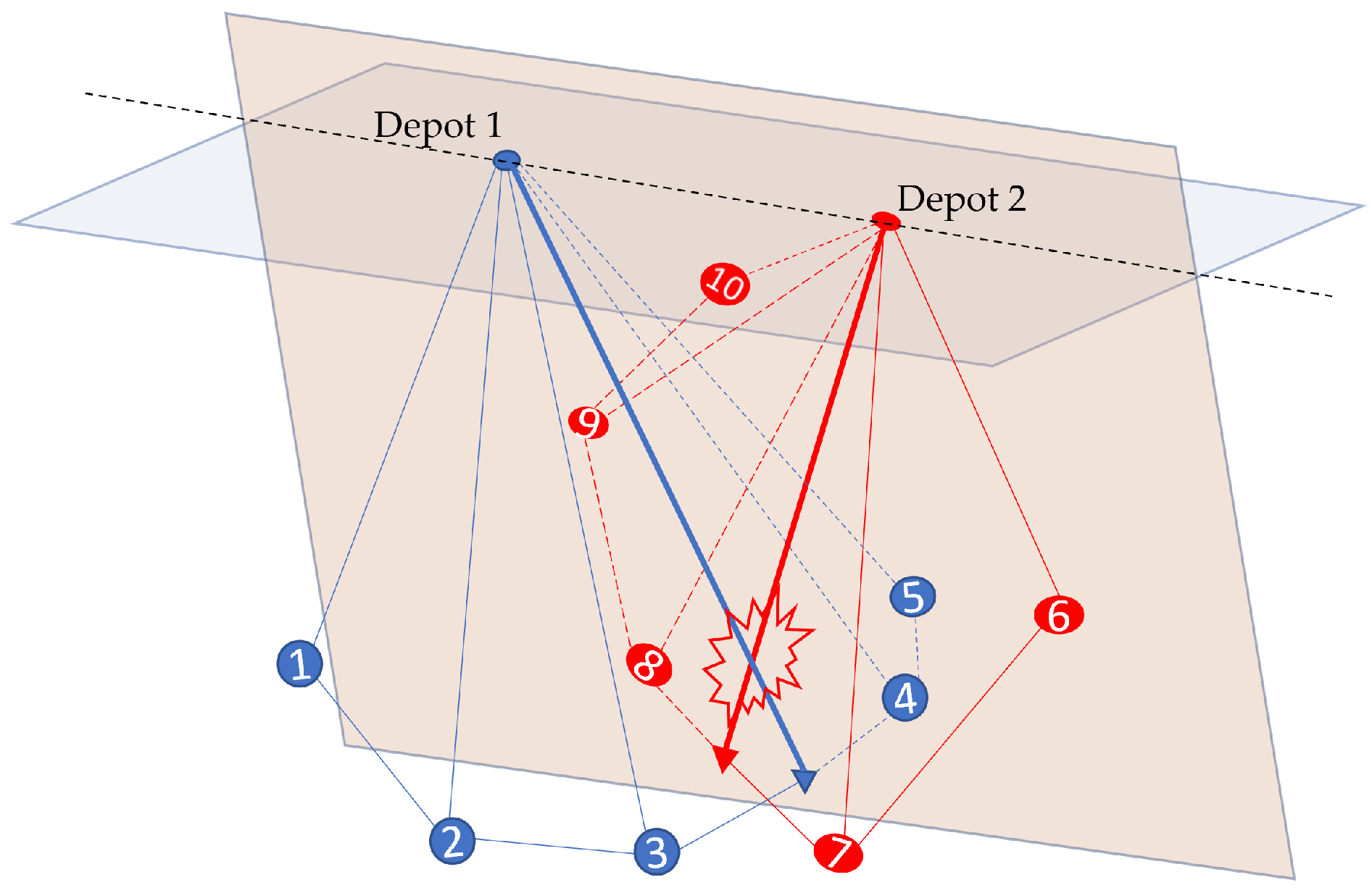
Algorithm 5 presents the overall steps to detect the possible entanglements and resolve the issue. When entanglement occurs, we can observe co-planer cable vectors, as shown in Figure 1. To inspect co-planer cable vectors for possible entanglement, the following equation is used:

$$\begin{array}{c}\hfill (\overrightarrow{C{V}_i^t}\times \overrightarrow{C{S}_{ij}})·\overrightarrow{C{V}_j^t}=0\end{array}$$

(7)

Algorithm 7 [Schedules, Time]=TimeScheduling($R_i,R_j$)

1: $R_{yield}\leftarrow R_i$ and $R_{pass}\leftarrow R_j$ 2: Select $n_{yield}$ from the nodes visited by $R_{yield}$ before the time of entanglement such that the cable vector at $n_{yield}$ does not intersect with the cable planes of $R_{pass}$ 3: Find a node $n_{pass}$ in route of $R_{pass}$ such that all the cable planes comprised of the nodes after $n_{pass}$ never intersect with any of the cable planes of $R_{yield}$ 4: $t_{yield}\leftarrow$ scheduled arrival time of $R_{yield}$ at $n_{yield}$ 5: $t_{pass}\leftarrow$ scheduled arrival time of $R_{pass}$ at $n_{pass}$. 6: $W\leftarrow t_{pass}-t_{yield}$ 7: $R_{yield}\leftarrow R_j$ and $R_{pass}\leftarrow R_i$ and repeat steps 1–6. 8: Choose $R_{yield}$, which incurs lower W 9: Return the adjusted schedules with the maximum tour time.

The value of t obtained upon solving (7) is the time after which the tethers are anticipated to entangle. If t is a positive real value within the range allowed by both vehicles’ schedules, the cables will become a co-planner and may become entangled if the cable segments intersect. Based on this fact, Algorithm 5 tries to find all possible entanglements within the initial routes. For a time interval between two consecutive departures $D_z$ and $D_{z+1}$, it simulates the movement of the vehicles and examines the concurrent cable planes. If entanglement is not detected, it selects vehicle P associated with $D_{z+1}$, updates $T_P$ and $S_k$, and examines the new cable plane of P against other concurrent cable planes using (7). The steps are repeated until either an entanglement is detected or the time interval associated with the last departure is passed without an entanglement. If entanglement is confirmed, it either modifies the existing routes based on Algorithm 6 or adjusts the time schedules based on Algorithm 7. The heuristic chooses the approach that resolves the entanglement at the expense of a lower maximum tour cost and accordingly updates the schedule or routes. Consequently, the algorithm re-initiates a fresh detection for an entanglement from the beginning at time $t=0$. As a last step, the algorithm only checks if the current solution is better than the solution only with time scheduling. This step is added because (1) the time scheduling only can run very fast, and (2) modifying the routes at the beginning causes a drastic delay in the final result for some cases.

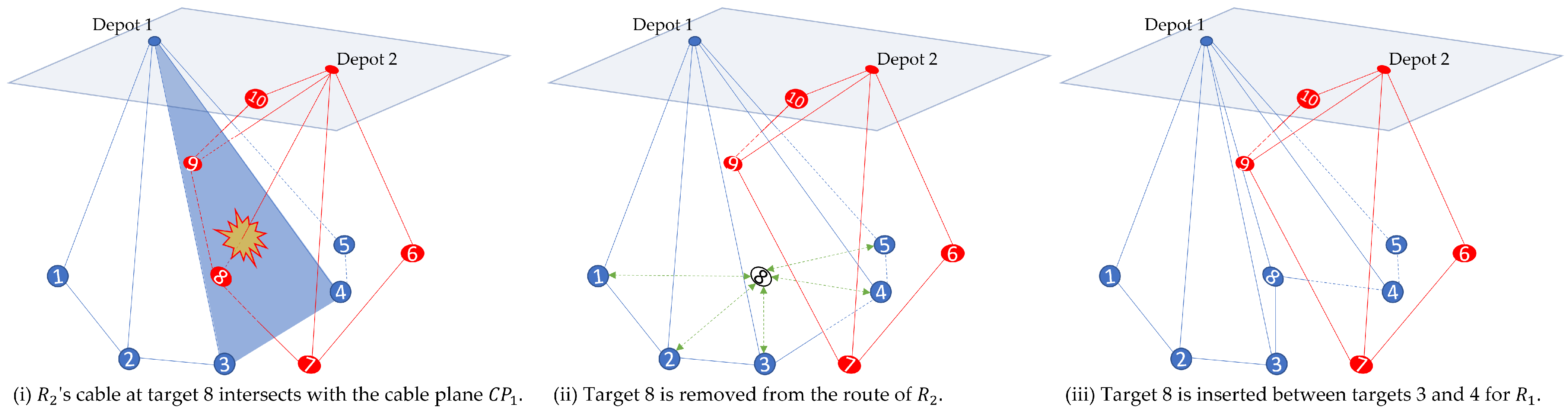
The route modification approach in Algorithm 6 tries to find alternate routes by reallocating the node relevant to the entanglement. For example, if the cable vector of $R_a$ intersects with $C{P}_b$, the responsible node is removed from $R_a$’s route and awarded to another vehicle with the lowest maximum tour time. Figure 2 shows how the approach works with an example. In this example, there is possible entanglement when $R_1$ travels between targets 3 and 4 while $R_2$ travels between targets 7 and 8 in the initial routes as shown in the far left figure. Thus, target 8 is removed from the route of $R_2$ and inserted for $R_1$ between targets 3 and 4.

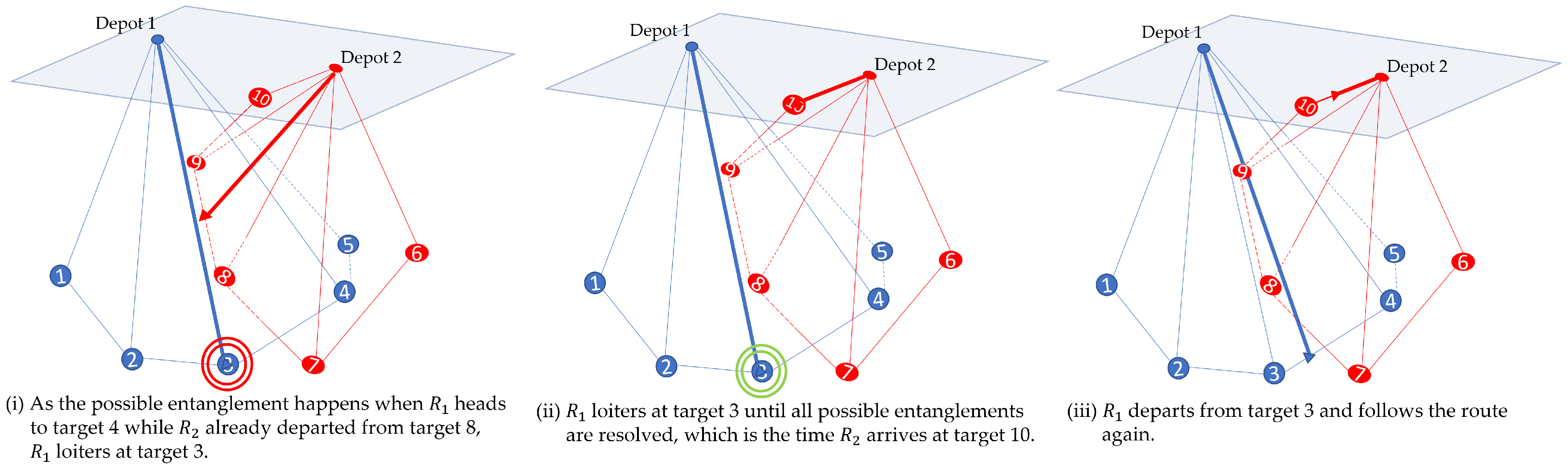
On the other hand, the time scheduling approach in Algorithm 7 adjusts the schedules while forcing one of the vehicles involved in the entanglement to loiter on the starting node on the plane involved in possible entanglement. It compares the loitering time to avoid entanglement and chooses a more efficient one. Figure 3 shows the rescheduling between the vehicles for the same example in Figure 2. There exists a possible entanglement when $R_1$ travels between targets 3 and 4 while $R_2$ travels between targets 7 and 8. As $R_2$ leaves the departing target earlier than $R_1$, $R_1$ waits at target 3 until all possible entanglements are resolved. Thus, $R_1$ restarts to follow the route when $R_2$ arrives at target 10.

The proposed heuristic approach produces a feasible solution for every case for the following reasons: (1) The primal-dual heuristic that produces the initial task allocation and routes guarantees a feasible solution without considering the entanglement constraint. (2) The proposed heuristic in Algorithms 5–7 ensures the removal of all the possible entanglements from the initial routes. Thus, all constraints are guaranteed to be satisfied, although the heuristic may not produce an exact optimal solution.

4. Computational Results

The heuristic is implemented and tested in simulations with varying problem sizes for validation. All simulations were performed on a PC with an Intel^®Core™ i7-7800X CPU running at 3.5 GHz with 64 GB RAM. The number of vehicles varied from 3 to 10, and the number of targets was tested for 50 and 100. The tests were repeated for 100 different instances for each problem size. The coordinates of targets and depots are randomly generated within a space of 2 m × 2 m × 3.2 m with a uniform distribution. All the depots are constrained to lie in the topmost plane of the defined space. All vehicles had the same average running speed. $Cos{t}_{ij}^k$ was set to the minimum travel time by calculating the distance between i and j divided by the average running speed.

The maximum tour time among all vehicles is considered the operation time. The experiment evaluates the efficacy of the proposed algorithm to provide entanglement-free navigation of the vehicles while aiming to curb the increase in operation time. Due to a lack of available literature on this problem, we have computed posteriori bounds $P{B}_1$ based on the upper and lower bounds utilizing the initial routes produced by the primal-dual heuristic. The worst feasible solution is one vehicle departing at a time, and all other vehicles waiting until the vehicle comes back to its depot. For this trivial approach, the operation time is calculated by adding up the respective tour times of all the vehicles, and we consider this as the upper bound. On the other hand, the initial operation time produced by the primal-dual heuristic without considering the entanglement constraints is considered the lower bound, which is sometimes impossible to achieve. The equation we used to compute $P{B}_1$ is as follows:

$$\begin{array}{c}\hfill P{B}_1=(T_{algo}-T_{LB})÷(T_{UB}-T_{LB})\end{array}$$

(8)

where $T_{LB}$ represents the lower bound, $T_{UB}$ represents the upper bound, and $T_{algo}$ represents the operation time of the entanglement-free solution produced by the algorithm applied. While this becomes one way to estimate the qualities of solutions, we observed that the upper bound increases significantly as the problem size increases because each vehicle must wait a long time at its depot for other vehicles to complete their missions. Thus, we also computed posteriori bounds $P{B}_2$, only compared with the lower bound as follows:

$$\begin{array}{c}\hfill P{B}_2=T_{algo}÷T_{LB}\end{array}$$

(9)

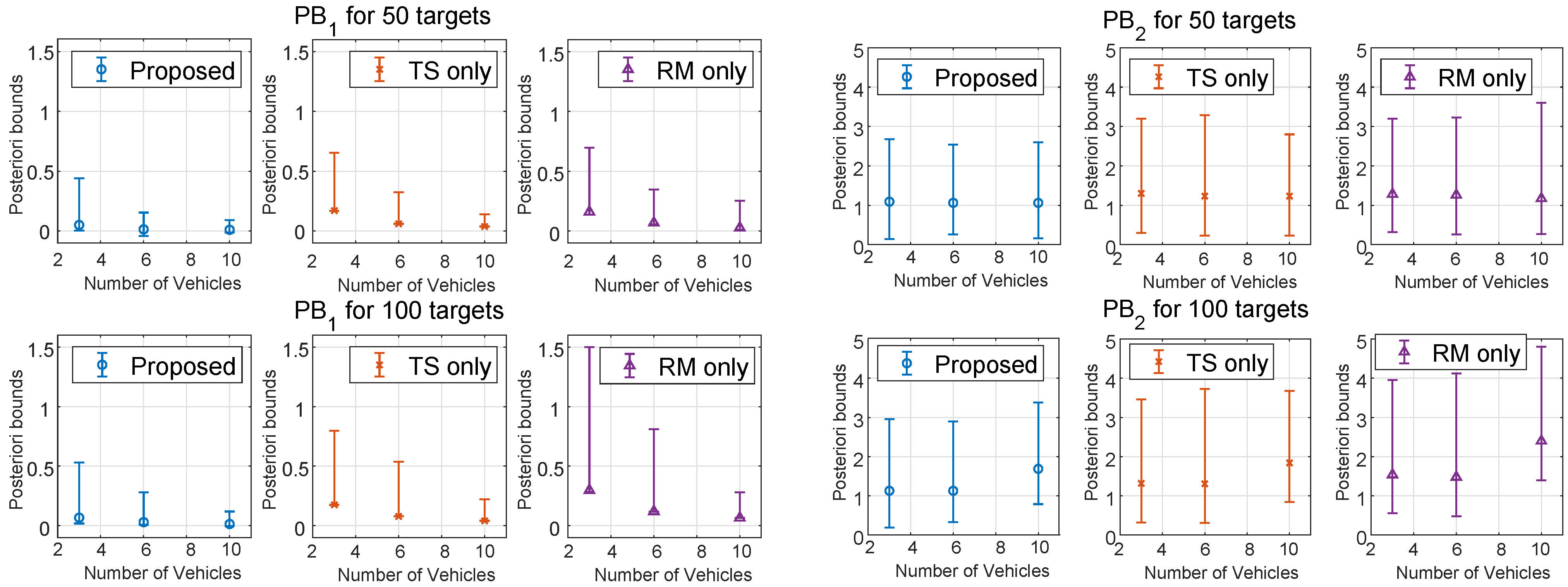
While the proposed algorithm uses a mixed approach between the rescheduling and route modification depending upon the cost, each problem instance is also solved only using one approach to compare the efficacy of both methods individually. The computational results are shown in Figure 4, and

Table 1. Computation time in seconds.

The Computation Time for the Entire Process
Vehicles	Proposed	TS	RM	Proposed	TS	RM
	Average with 50 targets			Worst with 50 targets
3	0.56	0.48	3.54	1.39	1.34	10.81
6	1.15	1.07	3.98	2.79	2.49	9.46
10	1.97	1.83	4.08	4.04	3.17	8.66
	Average with 100 targets			Worst with 100 targets
3	2.69	2.39	25.19	4.47	3.28	89.07
6	6.56	6.11	28.77	9.99	7.53	112.78
10	11.66	10.84	30.09	21.78	17.56	92.14
The computation time for entanglement resolving only
Vehicles	Proposed	TS	RM	Proposed	TS	RM
	Average with 50 targets			Worst with 50 targets
3	0.1	0.02	3	0.55	0.1	10
6	0.13	0.17	3	1.12	0.17	7
10	0.28	0.13	2.38	2.50	0.26	7
	Average with 100 targets			Worst with 100 targets
3	0.33	0.04	23	1.77	0.1	87
6	0.6	0.1	23	3.5	0.46	105
10	1.06	0.23	19	6.8	0.6	77

.

In Figure 4, the left shows $P{B}_1$, comparing the gaps to the lower bounds with gaps between the upper and lower bounds. The right presents $P{B}_2$, comparing the costs with the lower bounds. The marker shows the average, while the bar shows the minimum and maximum values. In both figures, RM represents the route modification approach, and TS represents the time scheduling approach. The proposed approach is a hybrid of the two approaches. The average posteriori bounds for the proposed approach had the best solution quality among the compared methods while staying considerably closer to the minimum. This means that the results are consistent most of the time while only occasionally having some poorer cases. For $P{B}_1$, the minimum bounds for the proposed and route modification-only methods have negative and less than 1 values, showing that the routes are improved by modification of the initial routes provided by the primal-dual heuristic, which is used as the lower bound. While the solution quality stayed consistent for 50 targets, the largest problem size had some increased gap from the lower bound for the proposed method. This makes sense as the number of vehicles and targets increase, and more entanglement issues can arise from the initial routes. The route modification-only method had the worst performance and the longest computation time. This method tries to remove all the possible crossing surfaces by exchanging nodes, resulting in having an overloaded vehicle with high computation time in some cases. 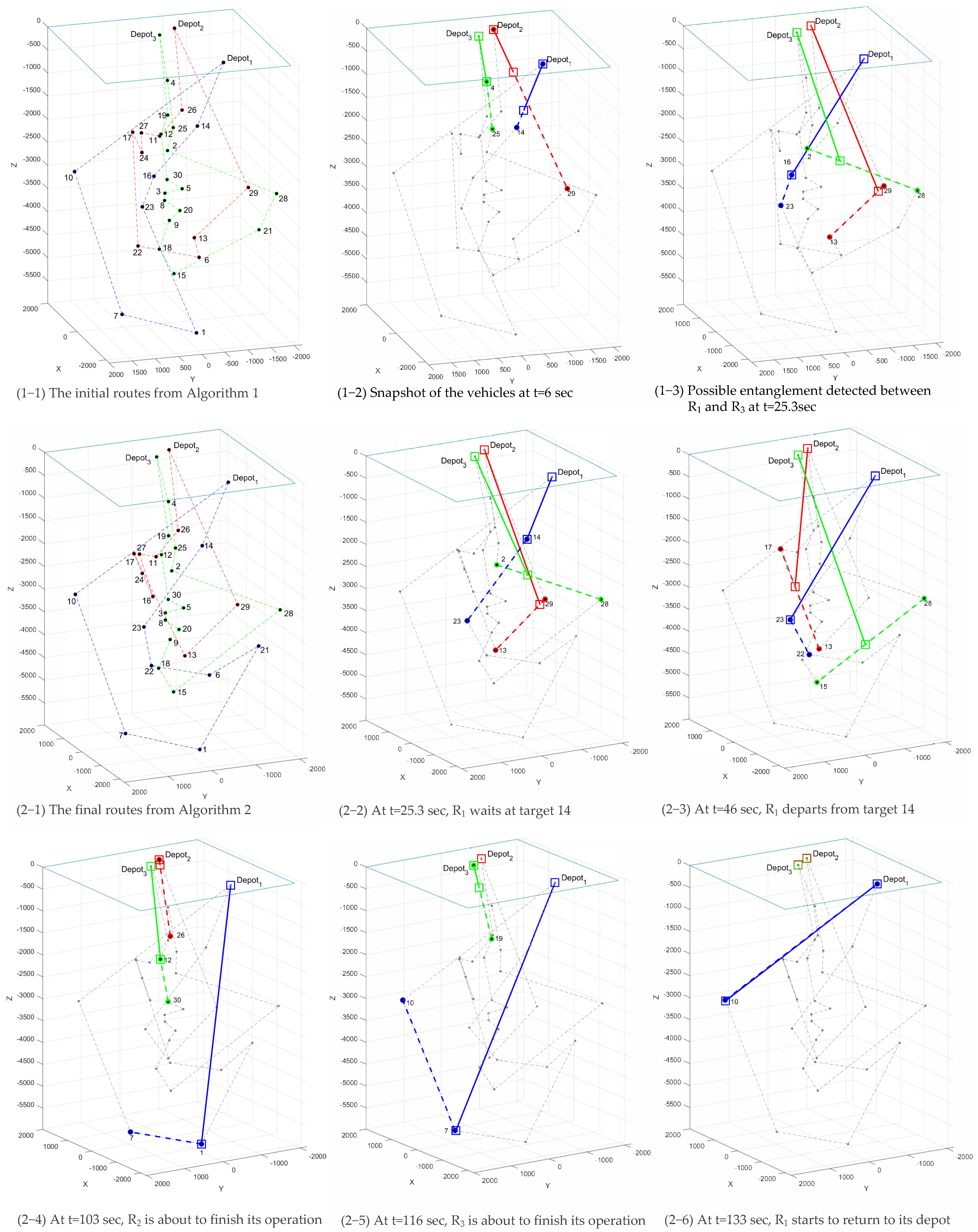While the time scheduling-only method solves the problem instantly, in less than 1 s for all cases, as shown in Table 1, the solution qualities were not as good as the proposed approach because some vehicles often need to loiter for a long time to resolve the entanglement issues. Thus, the proposed approach took advantage of both methods and produced the best solutions among the methods within a reasonable computation time. Although it compares the two methods every time it detects a possible entanglement, the proposed method’s computation time is considerably shorter than the route modification-only method because changing the route at a certain iteration changes the rest of the schedules. Therefore, the number of possible entanglement changes depending on which method was chosen in the previous step and affects both solution quality and computation time. The computational results show the algorithm’s potential to be implemented in real-world applications, delivering an affordable solution within an average of 11.66 s for the largest problem size, staying less than 1.5 of the ratio from a lower bound that does not consider the entanglement. Lastly, Figure 5 shows an example instance with 3 vehicles and 30 targets. As the possible entanglement is detected for the initial routes produced by Algorithm 1, Algorithm 5 updated the routes to avoid entanglements. As shown in Figure 5 of 1-1 and 2-1, some targets were exchanged between the vehicles while time scheduling was also performed in 2-2.

5. Conclusions

This paper presented an initial exploration of the problem of task allocation, path planning, and scheduling for T-AUVs. The proposed two-step heuristic algorithm efficiently allocates tasks among the vehicles, minimizing the last task completion time to ensure the production of non-entangling routes. Implementation results in simulation environments have demonstrated the effectiveness and potential of the algorithm, highlighting its capabilities for future extensions. While this study focused on simulation testing, our future work aims to perform field experiments using four BlueROV2 vehicles in a diving pool and at Lake Superior. These experiments will incorporate dynamic features of the tethers and vehicles into the algorithm, enabling non-straight line shapes based on water conditions. By including these dynamic elements, we can further validate the algorithm’s performance in real-world scenarios. Moving forward, we will address the challenge of incorporating the entanglement constraint into the problem formulation, ensuring it is considered simultaneously during algorithm design. Additionally, we plan to introduce heterogeneity among the vehicles, including subsets of vehicles without tethers or vehicles with different capabilities and motion constraints. By considering these variations, we can enhance the algorithm’s adaptability to diverse operational scenarios. This paper represents a preliminary step in coordinating T-AUVs for entanglement-free navigation. The outlined future extensions and considerations will contribute to a more comprehensive and practical solution for real-time applications in underwater environments. By addressing these complex challenges, we aim to facilitate the deployment of T-AUV systems in a wide range of underwater tasks, including ecosystem exploration, infrastructure inspection, maintenance, search and rescue, underwater construction, and surveillance.