Path Following for an Omnidirectional Robot Using a Non-Linear Model Predictive Controller for Intelligent Warehouses

Abstract

This paper presents results coming from a non-linear model predictive controller used to generate optimized trajectories specifically for an omnidirectional robot equipped with a spraying unit to mark on the floor the perimeter of dangerous areas or to move large palletized goods inside warehouses. Results on different trajectories and with moving obstacles are provided along with considerations on the controller performance.

1. Introduction

In recent decades, the growing demand for online purchases mostly coming from e-commerce and auction websites has led many companies to introduce robotics and technology systems in their warehouses as a way to increase their manufacturing productivity [1,2,3,4]. As a direct result, there has been a significant improvement to all the shipment services, since most couriers are now able to provide same-day delivery option [5] almost everywhere in the world. Obviously, in such context, it becomes very critical for modern warehouses to optimize all the logistics processes [6,7]. This is important, for example, to handle the goods when they are arranged on pallets [8,9] in order to reduce the probability of possible errors made by human operators, to relieve them from repetitive and monotonous tasks and, above all, to reduce the risk of employee injuries [10] that usually can occur while handling tasks that require lifting and turning of large or heavy packages in confined spaces. Thanks to the advances in the sensor technology [11] and the more remarkable innovations in the robotics field [12], some companies have been able to introduce mobile robots with automated systems [13] to handle the transport of oversized and heavy items in their warehouses, resulting in faster process times in the facility. Therefore, path following is a critical functionality for autonomous robots when the unit is required to move over a specified path with time constrains [14,15]. However, in realistic applications, the traditional methods for the control of mobile robots and vehicles often do not provide significant results [16,17] because of the complex setup used for the navigation algorithms and routines. This research work aims to describe the results coming from the application of a non-linear model predictive control (NMPC) used to implement a path planning application on a four-mecanum-wheeled omnidirectional robotic unit moving in dynamic environments. Section 2 includes detailed information about Omnibot, a mobile platform equipped with a sprayer unit that can be used, for example, to mark lines on the floor to delimit dangerous areas or to move large palletized goods inside the warehouses in addition to a description of the predictive controller as briefly described in [18]. Section 3 presents the results coming from the MATLAB simulations, while Section 4 concludes the paper.

2. Materials and Methods

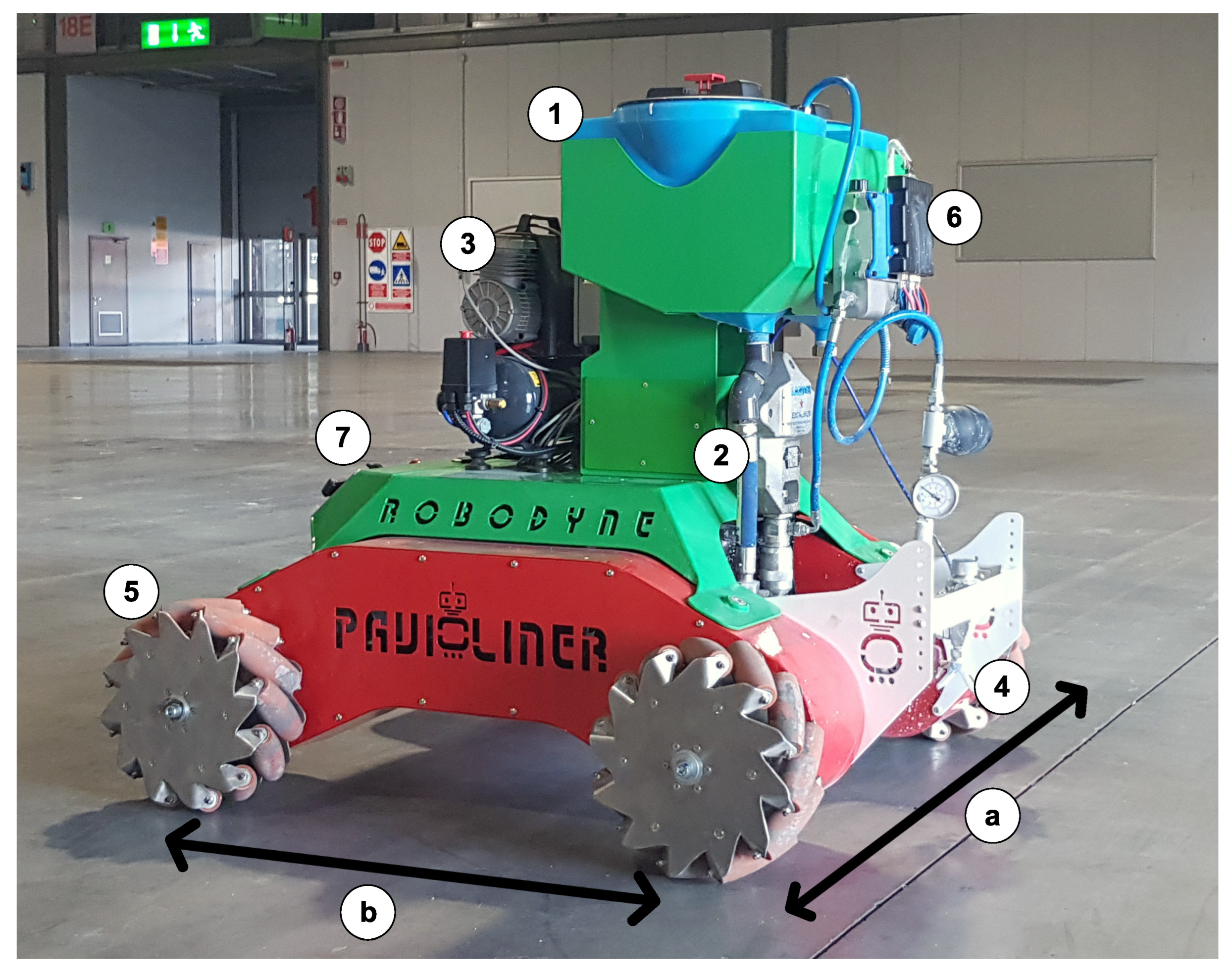
2.1. The Omnidirectional Robot

Figure 1 highlights all the main characteristics of Omnibot, the four-wheeled omnidirectional robot used for this research work. This mobile unit has a total length of $b=1012$ and a total width of $a=1038$ mm to provide a large upper surface for add-ons and external devices. Each mecanum wheel (5) is directly coupled with a 500 W brushed DC motor that can spin up to 3000 rpm and with a worn gearbox having a reduction ratio $i=30$; each electric motor integrates an optical encoder with 1024 pulses, which is mainly used to provide an efficient and robust locomotion system and odometry [19].

The electronics system installed on board the robot relies on four controllers from Roboteq capable of commanding each single DC motor in PWM mode; moreover, due to their advanced 32 bit micro-controller, they can perform advanced motion control algorithms both in open- and closed-loop modes for speed and position by reading the measurements coming from the quadrature encoders. A very high-capacity battery pack including two sealed 12 VDC 200 Ah AGM batteries was installed on the bottom side of the robot to deliver a maximum output power of 4.8 kW protected by a 350 A battery isolator switch that integrates a high-load solenoid. Each mecanum wheel has a vertical load capacity of 250 kg, and the metal frame of the robot has a total payload of 1000 kg to allow for the use of large and heavy equipment in industrial environments (i.e., in this research work, the unit was equipped with a portable spraying unit). The robot was completely designed from scratch starting from a CAD design, made in Solidworks, and all the parts were manufactured by using laser cut and bending machines. The vehicle uses an airless spraying system powered by a hydraulic pump (2), commanded by a motor driver (6) that sucks out the paint stored in two upper tanks (1) and feeds it to a bottom nozzle (4) usually placed 25 cm away from the floor even if its height can be adjusted by using the positioning holes available on the nozzle support. Finally, an external 12 VDC air compressor (3) is used to enable or to disable the nozzle (4). The entire system can be powered on and off by using the main control panel (7), which also provides an emergency switch and multiple power connectors to plug additional devices.

Table 1. Technical specifications for Omnibot.

Omnibot Specifications	Value
Driving mode	holonomic with mecanum wheels
Total driving motors	4
Dimensions (a × b)	1012 × 1038 mm
Maximum velocity (any direction)	1 m/s
Maximum Payload	1000 kg
Output power	4800 W
Total weight	200 kg

reports the main mechanical specifications for the presented omnidirectional platform. An omnidirectional platform was selected over other configurations such as tank steering because mecanum wheels minimize the slipping effect on flat surfaces as well as the vertical vibrations on the frame [20].

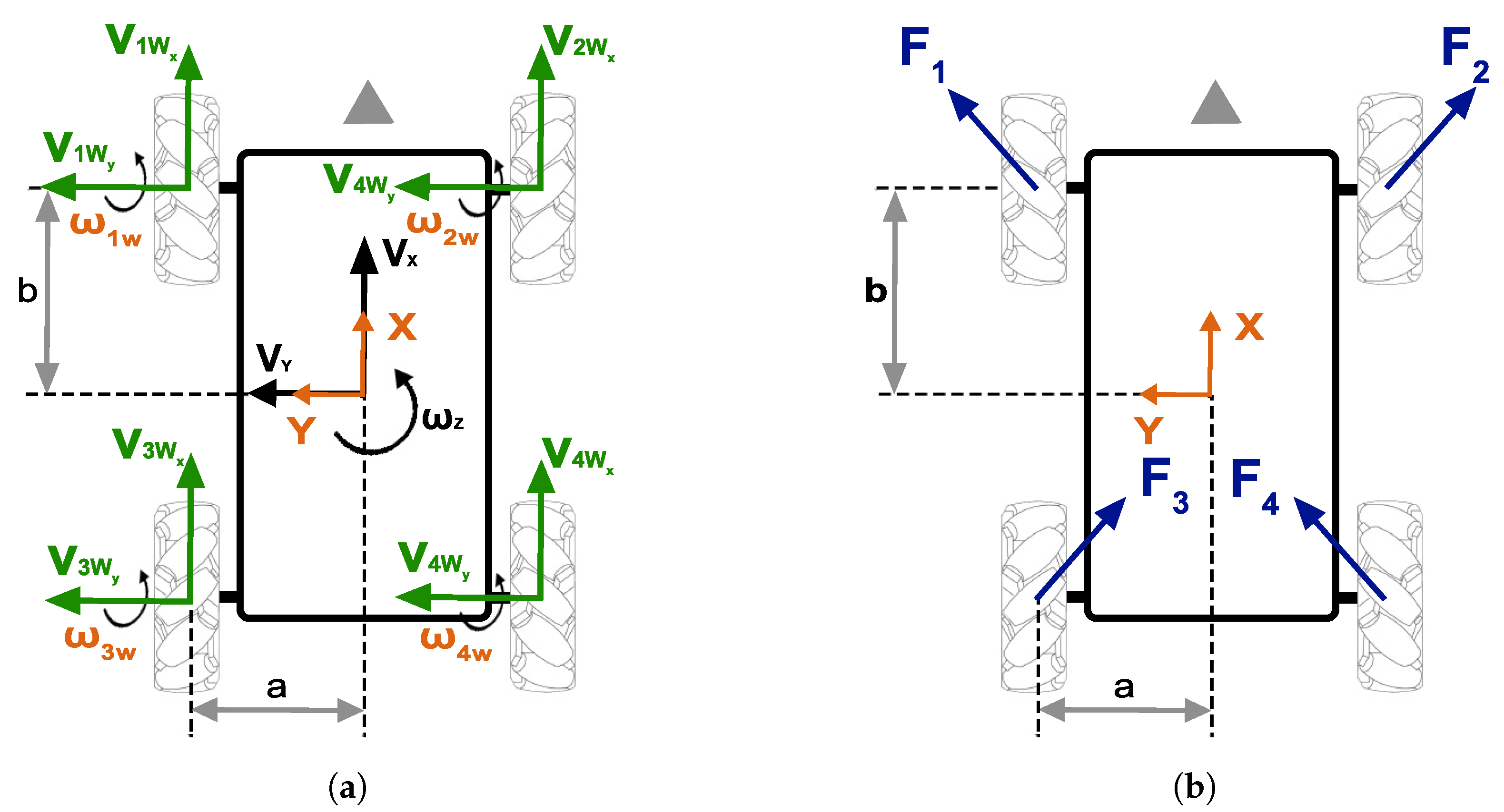
2.2. The Robot Model

An omnidirectional robot made up of a rigid body and non-deforming mecanum wheels is considered as reported in Figure 2a, where the main reference frame (X,Y) is coincident with its geometric center. By following this reference, it is possible to write the velocities for each wheel’s center as:

$$\begin{array}{c}\hfill V_{1W_Y}=V_{2W_Y}=V_Y+w_{z}b\\ \hfill V_{3W_Y}=V_{4W_Y}=V_Y-w_{z}b\\ \hfill V_{1W_X}=V_{3W_X}=V_X-w_{z}a\\ \hfill V_{2W_X}=V_{4W_X}=V_X+w_{z}a\end{array}$$

(1)

where b is the distance between the wheel hub and the geometric center of the robot along the X axis, a is the distance between the center of the wheel and the geometric center of the robot along the Y axis, $V_{i{W}_Y}$ is the i-th velocity of each wheel along the Y axis, and $V_{i{W}_X}$ is the i-th velocity of each wheel along the X axis.

The mecanum wheels consist in a series of twelve small rollers placed at $45deg$ from the axis of rotation; for this reason, it is necessary to take into account the equations for the i-th roller’s rotational velocity defined as:

$$\begin{array}{c}\hfill w_{iR}{R}_{R}sin\left({\alpha }_i\right)=V_{i{W}_Y}\\ \hfill w_{iR}{R}_{R}cos\left({\alpha }_i\right)=V_{i{W}_X}-w_{iW}(R_W-R_R)\\ \hfill w_{iW}=\frac{V_{i{W}_X}-V_{i{W}_Y}cotg\left({\alpha }_i\right)}{R_W}\end{array}$$

(2)

where $w_{iR}$ is the rotational velocity of the i-th roller around the $Z^{\prime }$ axis, and $R_R$ is the radius of each roller, ${\alpha }_i$ is its angular displacement from the axis of rotation, $w_{iW}$ is the rotational velocity for each wheel, $R_W$ is the radius of each mecanum wheel. Because of these relations, it is possible to rewrite the velocity of each wheel as follows:

$$\begin{array}{c}\hfill w_{1W}=\frac{1}{R_W}(V_X-V_{Y}cotg\left(\alpha \right)-w_Z(a+bcotg\left(\alpha \right)))\\ \hfill w_{2W}=\frac{1}{R_W}(V_X+V_{Y}cotg\left(\alpha \right)+w_Z(a+bcotg\left(\alpha \right)))\\ \hfill w_{3W}=\frac{1}{R_W}(V_X+V_{Y}cotg\left(\alpha \right)-w_Z(a+bcotg\left(\alpha \right)))\\ \hfill w_{4W}=\frac{1}{R_W}(V_X-V_{Y}cotg\left(\alpha \right)+w_Z(a+bcotg\left(\alpha \right)))\end{array}$$

(3)

By considering the matrix notation, the wheels velocity can be defined as:

$$\begin{array}{c}\hfill w_W=JV\end{array}$$

(4)

where:

$$W_W=\left[\begin{array}{c}{w}_{1W}\\ w_{2W}\\ w_{3W}\\ w_{4W}\end{array}\right],J=\frac{1}{R_W}\left[\begin{array}{ccc}1& -cotg\left(\alpha \right)& -(a+bcotg(\alpha \left)\right)\\ 1& cotg\left(\alpha \right)& (a+bcotg(\alpha \left)\right)\\ 1& cotg\left(\alpha \right)& -(a+bcotg(\alpha \left)\right)\\ 1& -cotg\left(\alpha \right)& (a+bcotg(\alpha \left)\right)\end{array}\right],V=\left[\begin{array}{c}{V}_X\\ V_Y\\ w_W\end{array}\right]$$

(5)

For convenience, by introducing the inverse matrix $\tilde{J}={\left(J^{T}J\right)}^{-1}{J}^T$ where:

$$\tilde{J}=\frac{R_W}{4}\left[\begin{array}{cccc}1& 1& 1& 1\\ -tg\left(\alpha \right)& tg\left(\alpha \right)& tg\left(\alpha \right)& -tg\left(\alpha \right)\\ 1& cotg\left(\alpha \right)& -(a+bcotg(\alpha \left)\right)\\ \frac{-1}{a+bcotg\left(\alpha \right)}& \frac{1}{a+bcotg\left(\alpha \right)}& \frac{-1}{a+bcotg\left(\alpha \right)}& \frac{1}{a+bcotg\left(\alpha \right)}\end{array}\right]$$

(6)

the linear $V_X$, $V_Y$ and the angular velocities $w_Z$ of the omnidirectional robot can be described as:

$$\begin{array}{c}\hfill V_X=\frac{R_W}{4}(w_{1W}+w_{2W}+w_{3W}+w_{4W})\\ \hfill V_Y=\frac{R_{W}cotg\left(\alpha \right)}{4}(-w_{1W}+w_{2W}+w_{3W}-w_{4W})\\ \hfill w_Z=\frac{R_W}{4(a+bcotg(\alpha \left)\right)}(-w_{1W}+w_{2W}-w_{3W}+w_{4W})\end{array}$$

(7)

In this specific case, the previous equations can be further simplified since the angle $\alpha =45deg$, and thus, $cotg\alpha =1$.

Since the wheels and their rollers have negligible mass compared to the total mass of the robot, it is possible to neglect the contribution of their inertia as well as the rolling resistance. Therefore, by adopting the Newton–Euler formulation derived by Newton’s second law of motion, it is possible to describe the dynamic system of the robot in terms of force and momentum. The robot can rotate about the Z axis and move along the X axis while it moves forward, and along the Y axis when it moves sideways. Newton’s equations of motion can be characterized as follows:

$$M\ddot{X}=M\dot{V_X}=\sum _{i=1}^4{F}_{iWX}=F_{1WX}+F_{2WX}+F_{3WX}+F_{4WX}$$

(8)

$$M\ddot{Y}=M\dot{V_Y}=\sum _{i=1}^4{F}_{iWY}=F_{1WY}+F_{2WY}+F_{3WY}+F_{4WY}$$

(9)

$$J\dot{w_z}=b(F_{1WY}+F_{2WY}-F_{3WY}-F_{4WY})+a(-F_{1WX}+F_{2WX}-F_{3WX}+F_{4WX})$$

(10)

$$T_{i}i{\mu }_r=F_{iWX}{R}_W$$

(11)

where $F_{iWX}$ is the i-th force acting along the X axis, $F_{iWY}$ is the force acting along the Y axis while $w_z$ is the angular velocity of the robot, $T_i$ is the torque of the i-th DC motor, $i=30$ is the gearbox reduction, and ${\mu }_r$ is the powertrain efficiency.

$$F_{iWX}=F_{z^{\prime }}sin{\alpha }_i$$

(12)

$$F_{iWY}=F_{z^{\prime }}cos{\alpha }_i$$

(13)

where $F_z^{\prime }$ is the axial force acting on the $Z^{\prime }$ axis on each roller. Depending on the relations between $F_i$, the robot can have different motion directions. However, it holds that it is possible to define the relations as $F_{1wY}=F_{1wX}$, $F_{2wY}=-F_{2wX}$, $F_{3wY}=-F_{3wX}$, $F_{4wY}=F_{4wX}$. All the previous considerations can be adopted to define the model of the robot in MATLAB to run the non-linear model predictive control. In matrix notation, the system is expressed as:

$$\dot{V}=f(V,T)$$

(14)

2.3. The Predictive Controller

Over the years, the controls used in robotics systems have dramatically changed to allow for more complex and dynamic non-linear actions. Modern applications involve dynamic environments with moving obstacles in the presence of human operators. Since picking and moving goods is a very critical task in warehousing accounting for about 50% of the overall operating costs [21], logistics robots play a key role in the process of building an intelligent warehouse. The optimization of the picking path allows the robot to easily reach items placed across thousands of square feet of the warehouse by minimizing the routing length and time; in addition, a correct path planning algorithm cannot only save logistics robot operation time, but it can also decrease the energy consumption and wear of the moving robot by reducing its maintenance costs. All these considerations also apply in the presented marking on the floor application since Omnibot is required to follow a specific trajectory by minimizing the tracking error and the total traveled length. Traditional industrial control strategies such as PID control may not guarantee such features since robot models are usually highly non-linear, making control strategies more difficult. Model predictive control (MPC) is a strategy that enables these more complex behaviors since it allows the use of a model of the plant to make predictions about future plant outputs [22,23]. It solves an optimization problem at each time step to find the optimal control action that leads the predicted plant output to the desired reference as close as possible. The MPC controller is a more advanced method of process control with the ability to deal with the constraints used for MIMO systems (multiple inputs, multiple outputs) compared with the PID controller that has no knowledge about the constraints. An MPC can be considered as a multi-variable control algorithm that relies on an internal dynamic model of the process, a cost function J over the receding horizon [24], which is a time window for the prediction, and an optimization algorithm minimizing the cost function J using the control inputs.

$$\begin{array}{c}\hfill J=\sum _{i=1}^N{w}_{x_i}{\left(r_i-x_i\right)}^2+\sum _{i=1}^N{w}_{u_i}\Delta u_i^2\end{array}$$

(15)

where J is the cost function, $x_i$ are the controlled variables or system states, $r_i$ are the robot reference variables, and $u_i$ are the inputs expected by the robot or the manipulated variables, $w_{x_i}$ and $w_{u_i}$ are the weight coefficients chosen according to the requirements and are relative to $x_i$ and $u_i$, respectively. The above cost function J minimizes the error from a reference trajectory and the jerk caused by drastic deviations in the inputs. Figure 3 depicts a typical working scheme for MPC where the robot is in the current instant k and has a reference trajectory, in red, that must be followed for a given prediction time horizon p.

MPC receives the current states of the robot and simulates a number of combinations of control inputs for time from k to $k+p$ where p is obtained starting from the sample time. Among several possibilities, MPC selects the best set of inputs that minimizes the cost function J. Only the first step of this control strategy is implemented, then the system state is sampled again, and the calculations are repeated starting from the new current state $k+1$ up to $k+1+p$ with a new control and a new predicted state path. The prediction horizon continues to move forward with the same duration p, and for this reason, MPC is also called the receding horizon control (RHC).

2.4. Non-Linear Predictive Model Control (NMPC)

In general, MPC is one of only a few advanced control methods that are currently used successfully in industrial control applications, especially in those systems that can be sufficiently represented with a linear model. The growing use of this algorithm is justified by its ability to manage large-scale multi-variable processes with tens or hundreds of inputs and states that must satisfy physical and operational constraints. The operating principle of the MPC algorithm relies on the formulation and the solution of a numerical optimization problem corresponding to an optimal control problem with a finite time horizon p at each sampling instant k. Since the system state is updated during each sampling period, the receding horizon approach must be adopted; thus, a new optimization problem must be solved at each sampling interval. Linear models can be handled using a large variety of numerical and software methods since the MPC problem in those cases is typically a quadratic or linear program, which is known to be convex and thus can easily be solved. However, mobile robot kinematic models are non-linear affine systems constrained by velocity and acceleration limits. The non-linear model predictive control (NMPC) seems to be able to provide the possibility to operate with a non-linear system. As already explained in detail in [26,27], the NMPC controller has gained popularity in industrial applications because of its capability to explicitly take into consideration the constraints that can be specified both for the set of inputs (saturation constraints) and for the controlled variables y (i.e., to limit the overshoot value or to prevent non-minimal phase behaviors). All states are measured with a fixed sampling time $T_s$, and their values are provided to the NMPC algorithm with the same sampling to obtain a prediction of the system. At any moment, the control law determines a prediction of the states and of the outputs within an interval $[t,t+T_p]$ where $T_p$ is the prediction horizon. Then, the non linear controller estimates the expected output of the system according to both the initial state of that prediction interval $x\left(t\right)$ and the input for a specific instant of time in that interval. To reduce the computation, it is possible to assume that the input changes only for a time fraction of the prediction horizon, which is also called the control horizon, after which the input value remains constant. Both $T_p$ and $T_C$ are integer multiples of the sampling time $T_S$, while $u\left(t\right)$ is an open-loop input since it no longer depends on the initial state. The primary goal of this non-linear controller is to generate a prediction-based input that minimizes the cost function J. The NMPC control functionality and dynamic performance is typically provided by the cost function J and the constraints of the system. The optimization problem consists in minimizing at each sampling instant the squared-weighted norm of the tracking error, over a finite time interval. The other contributions in the cost function take into account the final tracking error and how the algorithm manages the trade-off between performance and command activity.

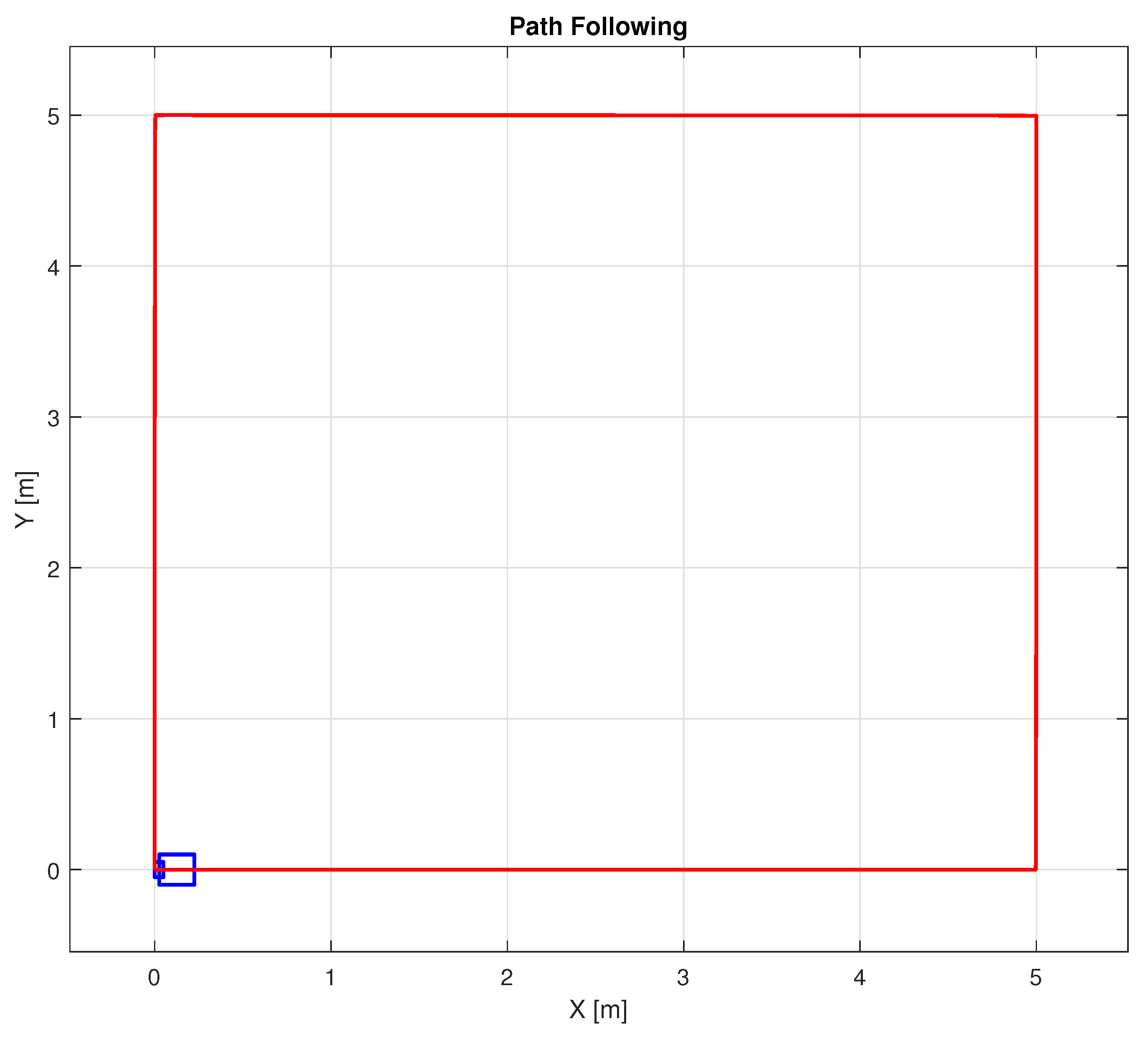
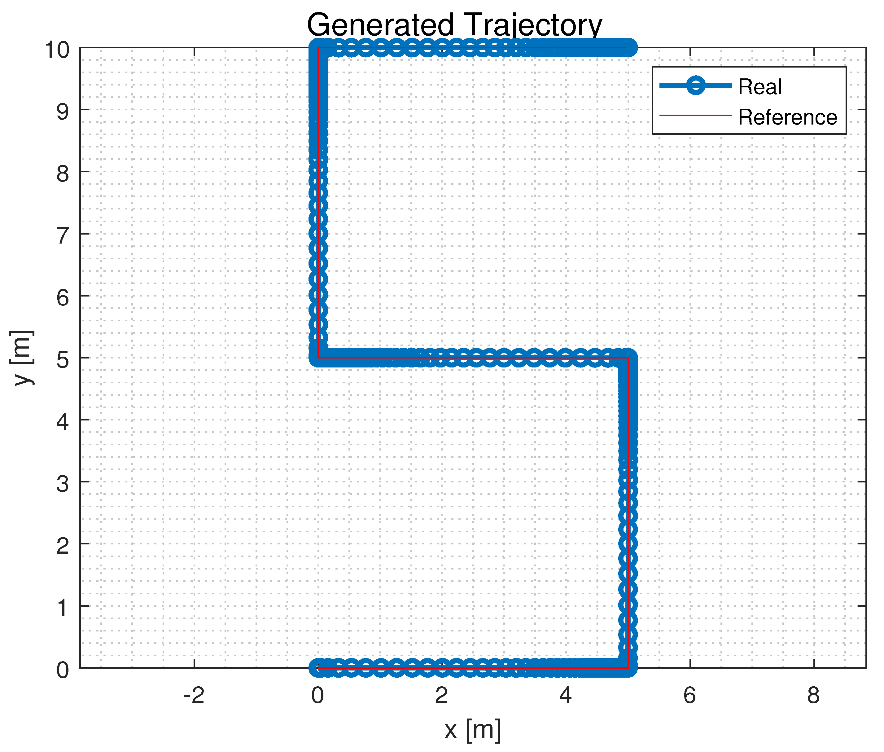
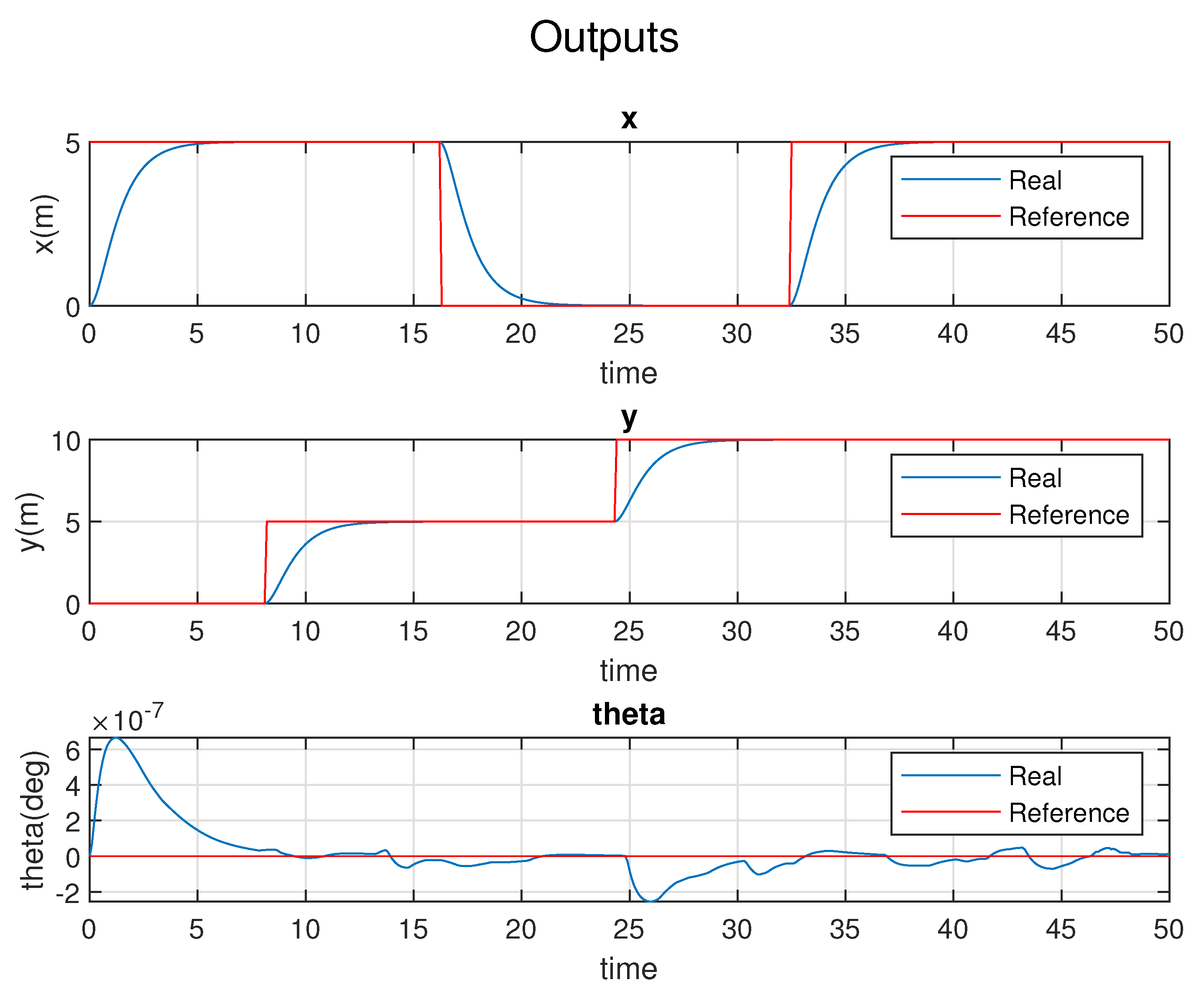
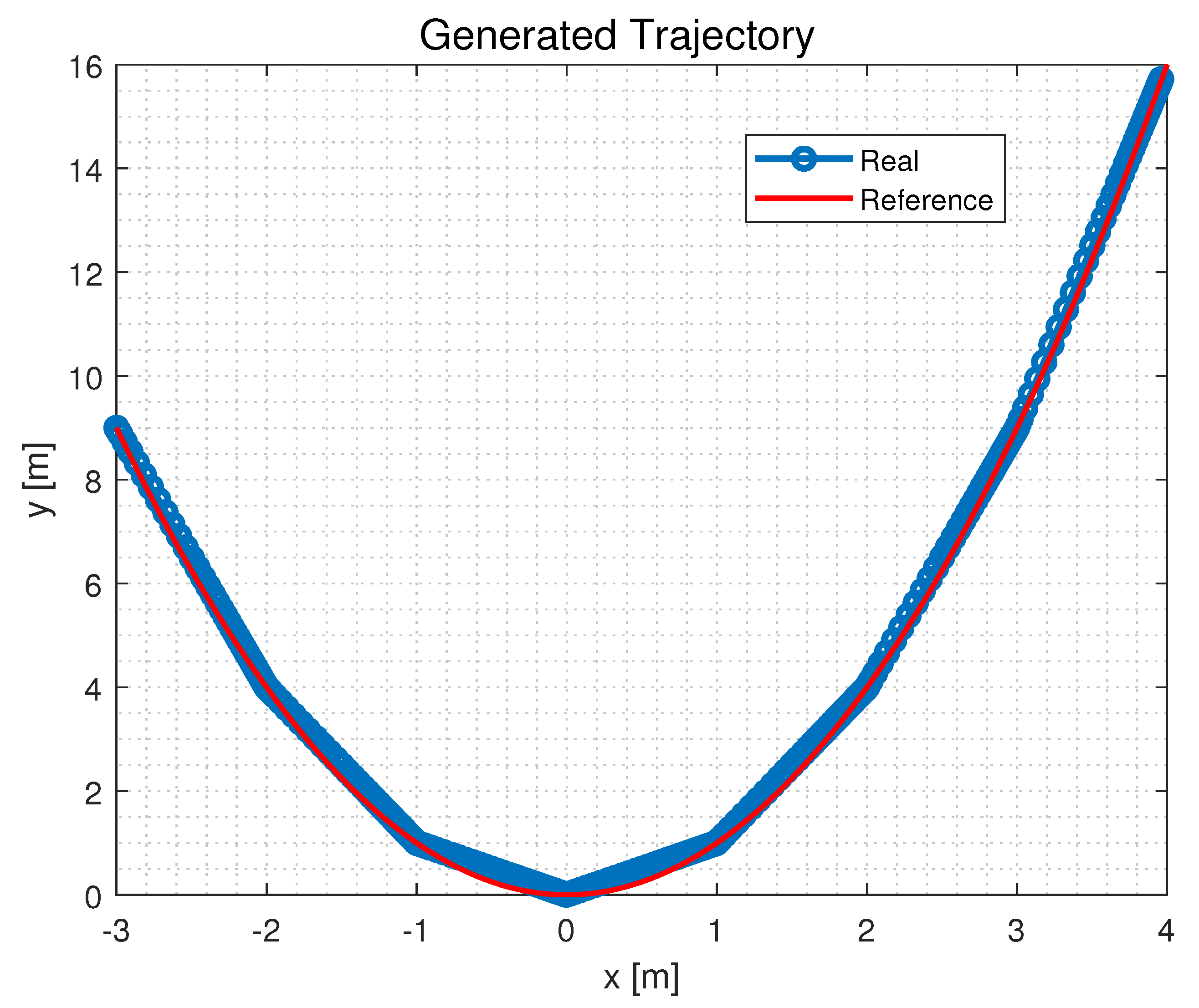
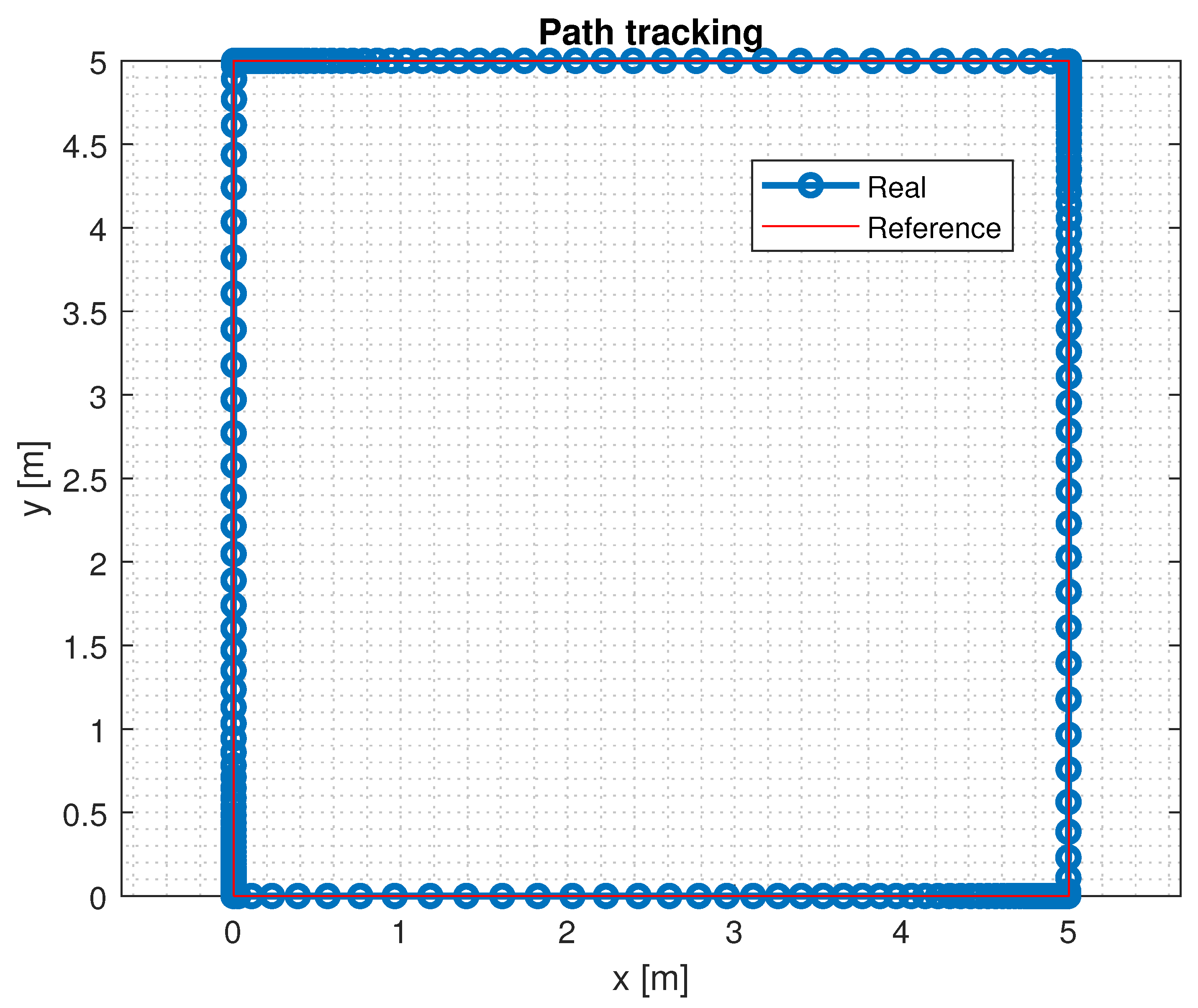
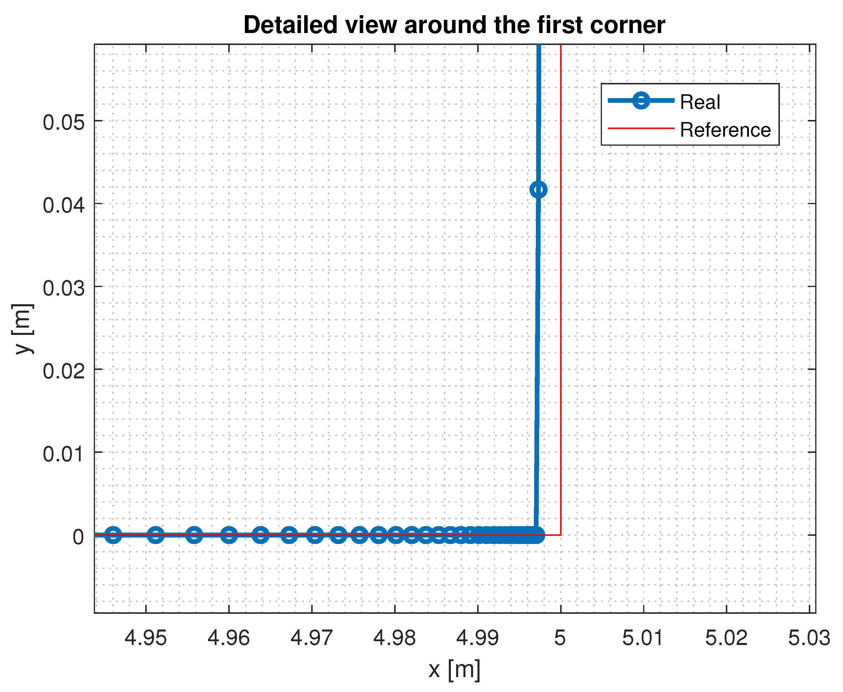
3. Results for the NMPC Algorithm

In order to test the performance of the NMPC over the dynamic model of the robot, MATLAB was used, since it allows for matrix manipulations, plotting of functions and data, implementation of algorithms, creation of user interfaces, and interfacing with programs written in other languages; in particular, it provides a non-linear MPC function to calculate control actions at each control interval using a combination of model-based prediction and constrained optimization. The real robot runs a ROS package that enables it to communicate with a server machine with a ROS master. The final user creates the reference path by using a third-party motion planner installed on the server whose output contains jumps in positions by default. For this reason, the reference path in Matlab was created with a similar behavior in order to test the controller in more realistic conditions. Before starting with the simulation tests, the controller was tuned trying different parameter and constraint configurations, always with a view focused on the real robot. In particular, for safety reasons, the real robot must have a maximum velocity of 0.5 m/s, and the output torque on each motor cannot exceed 15 Nm. Moreover, the robot is usually adopted to mark lines on the floor by using different colors, and for this reason, two or more tanks are installed on the upper frame and are filled with colored paint. When the task requires the robot to follow long trajectories, it can happen that its total weight decreases since the tanks gradually empty as the system uses the sprayer. The weight is known at the beginning of the task; however, it can dynamically change later, ranging from a minimum of 200 kg to a maximum of 1200 kg. Since the hardware used to process the algorithm is limited and there is no sensor to measure the weight variation onboard the robot, it is not possible to adjust the parameter of the controller on the fly. Consequently, the best controller is the one providing a good balance between performance and accuracy corresponding to different weights. At the beginning, the sampling time was set to 2 Hz since it is a good compromise between the electronics installed on board the robot and the overall performance of the controller; then, considering that each step of the prediction horizon is equal to the sampling time, a value around 18 steps was selected since the use of lower or higher values caused the failure of the path following the algorithm. Having low-performance hardware on board the robot is mainly for saving production costs, and the value for the control horizon was set shorter than the prediction horizon to save computational effort. However, making it too short may degrade control performance; thus, a value of 10 was selected, since lower values provide low performance, and values of about 14 have a negative impact on the calculation time. A total of ten tests for different controller configurations was performed to arrive at the best combination of parameters, i.e., the values of the constraints and weights relating to the manipulable variables, the weights relating to the output variables, that allows the omnidirectional robot to follow the desired trajectory specifically for the target application. For each simulation case, the RMS (root mean square) value was calculated to quantify the deviation between the points of the desired trajectory and those belonging to the real trajectory. Figure 4 shows a closed square trajectory used as reference for the path tracking tests. Figure 5 shows the generated trajectory used by setting the prediction horizon to 18 time samples and the control horizon to 5 time samples, with a sampling time of 0.1 s. Figure 6 reports the error deviation between the reference, in red, and the followed path, in blue, when the robot reaches the first corner. The controller evaluates the best trajectory depending on the constraints and the parameters, and during this simulation and quite the opposite of what would happen with the real robot, the measured distance along the X axis between these two paths is 0.006 m. It is possible to consider the reference path and the generated trajectory as coincident since they completely overlap at the other corners.

By leaving unchanged the prediction and the control horizon, a series of ten sets of tests were run by changing the values of the weight of the manipulated and output variables. The obtained results are reported in

Table 2. For all sets, a total of ten tests were performed for each parameter configuration where the test with the lowest RMS is considered to have the most suitable controller for the final application.

Set	Parameters	RMS (m) (Best Case)	RMS (m) (Worst Case)
1	$W_v=20$, $W_{vr}=1$, $W_{vo}=100$	0.1620	0.4310
2	$W_v=21$, $W_{vr}=2$, $W_{vo}=95$	0.1280	0.3150
3	$W_v=22$, $W_{vr}=1$, $W_{vo}=98$	0.1360	0.4810
4	$W_v=23$, $W_{vr}=3$, $W_{vo}=99$	0.1820	0.1710
5	$W_v=25$, $W_{vr}=1$, $W_{vo}=100$	0.1010	0.4210
6	$W_v=25$, $W_{vr}=2$, $W_{vo}=101$	0.1120	0.4280
7	$W_v=25$, $W_{vr}=1$, $W_{vo}=99$	0.1110	0.4280
8	$W_v=25$, $W_{vr}=2$, $W_{vo}=100$	0.1320	0.5220
9	$W_v=26$, $W_{vr}=1$, $W_{vo}=100$	0.1920	0.3710
10	$W_v=25$, $W_{vr}=1$, $W_{vo}=97$	0.2020	0.6330

along with their best and worst RMS values defined as:

$$d_{\mathrm{RMS}}=\sqrt{\frac{1}{N}\sum _{n=1}^N{\left|x_n\right|}^2}$$

(16)

The best result with the lowest RMS value was obtained during test 1 by setting $W_v=25$, $W_{vr}=1$ and $W_{vo}=100$, where $W_v$ is the weight of the manipulated variables, $W_{vr}$ is the weight of the manipulated variables rate, and $W_{vo}$ is the weight of the output variables. Even if the robot needs only to move along simple trajectories since the perimeters of dangerous areas inside warehouses are usually square shaped, the control algorithm was also tested on different paths; this is mainly because the robot can also be used for additional tasks such as move heavy palletized goods among different working areas inside large workshops. For instance, Figure 7 shows the generated trajectory obtained by adopting the combination of parameters as in Set 5, reported in Table 2, where the s-shaped reference path, in red, was used to generate the final trajectory, in blue. As it is also highlighted in Figure 8, the prediction control provides the same performance as in the previous closed path since the deviation error at the third corner is 0.01 m. Figure 9 highlights how the controller elaborates the output variables x, y, and $\theta$ according to the given reference path to keep the robot on the track by reducing the following error.

The controller was also tested on more complex paths such as the curved trajectory showed in Figure 10, which is characterized by a tight turning radius; it can be observed how, in this case, the controller is not able to deliver the same performance as in all the previous situations, since in the area where the curve is tighter within $-1<x<1$, the deviation error along the Y axis reaches 0.2 m, as can be seen in Figure 11. It was noted that the computational time significantly increases when the system is closer to the constraints, making the solution useless due to the time delay; this happens mostly when the weight of the manipulated variables is below 12 or above 80. With sampling rates above 4 Hz, the computational time was registered as greater than 240 s with an Intel Core i5 CPU and under 75 s for every simulation with the sampling time set at 2 Hz. Ideally, it can be observed that removing the constraints or moving up their values helps to obtain faster computational time and to reach a more steady velocity profile along the entire reference path.

Collision Avoidance

Even if the robot is supposed to run autonomously in an empty and obstacle-free environment while marking lines on the floor, a collision-avoidance system based on a Sick LMS-111 2D laser was considered to be installed in the geometric center of the robot itself. This is mainly because the robot, under some circumstances, can also be used to move large loads inside workshops and warehouses in the presence of moving objects, i.e., human operators or other autonomous machines. The laser sensor measures the distance to an obstacle in front of the robot and on the same trajectory; the obstacle can be static, such as a pillar, or a moving object. In both cases, the robot should temporarily move outside the generated trajectory, travel around the obstacle, and return to the original track. While, for path tracking, the cost function J as described in (15) has a direct relation with the tracking error between the actual position of the robot and the reference path, for obstacle avoidance, the cost function has an inverse relation with the distance between the obstacle and the frame of the robot. One of the most suitable and easy-to-implement algorithms for obstacle avoidance when using NMPC is the bug-type algorithm [28], where the robot is forced to move on the shortest path between its initial position and the target position until it detects an obstacle; when a detection occurs, the robot is commanded to move tangentially around the surface of the obstacle and then return to its original path only after having fully avoided the obstacle. The following relation was added to the formulation of the NMPC controller:

$$\begin{array}{c}\hfill \sqrt{{(x_r-x_o)}^2+{(y_r-y_o)}^2}>R_r+R_o\end{array}$$

(17)

where $x_r$ and $y_r$ are the coordinates that define the current position of the robot, $x_o$ and $y_o$ are the coordinates that define the position of the obstacle, $R_r$ is the radius used to define the safe area for the robot, and $x_o$ is the radius used to specify the collision and restricted area. Figure 12 shows the output trajectory generated again with the parameters, as in Set 5 in Table 2, by the NMPC controller in order to avoid an obstacle placed at $x=30$ m in front of the robot over a straight line; the red dashed circle defines the restricted area for the robot, and the black line is the new trajectory with the tangency condition over the collision circumference. Figure 13 shows some frames related to a simulation made in Matlab where the robot is commanded to move from its original position $x,y=(3,3)$ to the target position placed in $x,y=(0,0)$ by following a straight trajectory while moving among dynamic obstacles with different dimensions. In this case, the radius of the safety area for the robot was increased for security reasons and to save CPU time with the aim of decreasing the computation time, which usually results in predicting the system’s state over the specified horizon. Figure 14 shows the full trajectory with the main positions of the robot while avoiding the obstacle. In this last case, the time required to complete the task is very demanding and would probably be very challenging to test in a real environment.

4. Conclusions

This research work aimed to provide results on the performance obtained by the application of a non-linear model predictive control used to plan trajectories for an omnidirectional mobile robot used to mark on the floor the perimeter of dangerous areas inside warehouses. The results obtained by adopting different trajectories have been presented along with their RMS values used as comparison values to evaluate the effectiveness of the controller. Furthermore, the results with the implementation of the obstacle avoidance feature have been provided by considering the case of dynamic environments. Future work will surely focus on the direct application of this controller on a real robot to test its performance in a real industrial context.

References

1. Galati, R.; Mantriota, G.; Reina, G. Design and Development of a Tracked Robot to Increase Bulk Density of Flax Fibers. J. Mech. Robot. 2021, 13, 050903. [Google Scholar] [CrossRef]
2. Fernando, Y.; Mathath, A.; Murshid, M. Improving Productivity:: A Review of Robotic Applications in Food Industry. Int. J. Robot. Appl. Technol. 2016, 4, 43–62. [Google Scholar] [CrossRef]
3. David, W.; Rovida, F.; Fumagalli, M.; Krueger, V. Productive Multitasking for Industrial Robots. arXiv 2021, arXiv:2108.11471. [Google Scholar]
4. Galati, R.; Mantriota, G.; Reina, G. Adaptive heading correction for an industrial heavy-duty omnidirectional robot. Sci. Rep. 2022, 12, 19608. [Google Scholar] [CrossRef] [PubMed]
5. Voccia, S.; Campbell, A.; Thomas, B. The Same-Day Delivery Problem for Online Purchases 2015. Transp. Sci. 2017, 53, 167–184. [Google Scholar] [CrossRef]
6. Omoruyi, O. Competitiveness Through the Integration of Logistics Activities in SMEs. Stud. Univ.-Babes-Bolyai Oeconomica 2018, 63, 15–32. [Google Scholar] [CrossRef]
7. Mikušová, N.; Čujan, Z.; Tomková, E. Robotization of Logistics Processes. MATEC Web Conf. 2017, 134, 00038. [Google Scholar] [CrossRef]
8. Liu, Y.t.; Sun, R.z.; Zhang, T.y.; Zhang, X.n.; Li, L.; Shi, G.q. Warehouse-Oriented Optimal Path Planning for Autonomous Mobile Fire-Fighting Robots. Secur. Commun. Netw. 2020, 2020, 6371814. [Google Scholar] [CrossRef]
9. Duan, L.M. Path Planning for Batch Picking of Warehousing and Logistics Robots Based on Modified A* Algorithm. Acad. J. Manuf. Eng. 2018, 16, 99–106. [Google Scholar] [CrossRef]
10. Palleschi, A.; Hamad, M.; Abdolshah, S.; Garabini, M.; Haddadin, S.; Pallottino, L. Optimal Trajectory Planning with Safety Constraints. In Proceedings of the 2021 I-RIM Conference, Rome, Italy, 8–10 October 2021. [Google Scholar] [CrossRef]
11. Andreasson, H.; Grisetti, G.; Stoyanov, T.; Pretto, A. Sensors for Mobile Robots. arXiv 2022, arXiv:2206.03223. [Google Scholar] [CrossRef]
12. Balatti, P.; Fusaro, F.; Villa, N.; Lamon, E.; Ajoudani, A. A Collaborative Robotic Approach to Autonomous Pallet Jack Transportation and Positioning. IEEE Access 2020, 8, 42191–142204. [Google Scholar] [CrossRef]
13. Li, J.t. Design Optimization of Amazon Robotics. Autom. Control. Intell. Syst. 2016, 4, 48. [Google Scholar] [CrossRef]
14. Nguyen, H.; Rego, F.; Quintas, J.; Pascoal, A. A review of path following control strategies for autonomous robotic vehicles: Theory, simulations, and experiments. J. Field Robot. 2022, 40, 747–779. [Google Scholar] [CrossRef]
15. Hogg, R.; Rankin, A.; Roumeliotis, S.; Mchenry, M.; Helmick, D.; Bergh, C.; Matthies, L. Algorithms and sensors for small robot path following. In Proceedings of the 2002 IEEE International Conference on Robotics and Automation (Cat. No.02CH37292), Washington, DC, USA, 11–15 May 2002; Volume 4, pp. 3850–3857. [Google Scholar] [CrossRef]
16. Atyabi, A.; Powers, D. Review of classical and heuristic-based navigation and path planning approaches. Int. J. Adv. Comput. Technol. (IJACT) 2013, 5, 1–14. [Google Scholar]
17. Do, H.; Tehrani, H.; Yoneda, K.; Ryohei, S.; Mita, S. Vehicle path planning with maximizing safe margin for driving using Lagrange multipliers. In Proceedings of the Intelligent Vehicles Symposium (IV), Gold Coast City, Australia, 23–26 June 2013; pp. 171–176. [Google Scholar] [CrossRef]
18. Galati, R.; Mantriota, G.; Reina, G. Nonlinear Model Predictive Control Of Omnidirectional Robots Using A Spraying Unit. In Proceedings of the Jc-IFToMM International Symposium, Kyoto, Japan, 16 July 2022; Volume 5, pp. 103–109. [Google Scholar] [CrossRef]
19. Galati, R.; Mantriota, G.; Reina, G. Mobile Robotics for Sustainable Development: Two Case Studies. In Proceedings of the I4SDG Workshop 2021, IFToMM for Sustainable Development Goals, online, 25–26 November 2021; pp. 372–382. [Google Scholar] [CrossRef]
20. Galati, R.; Reina, G. Terrain awareness using a tracked skid-steering vehicle with passive independent suspensions. Front. Robot. AI 2019, 6, 46. [Google Scholar] [CrossRef]
21. Andrejic, M.; Kilibarda, M.; Pajić, V. A framework for assessing logistics costs. In Quantitative Models in Economics; University of Belgrade: Beograd, Serbia, 2018; pp. 361–377. [Google Scholar]
22. Li, J.; Ran, M.; Wang, H.; Xie, L. MPC-based Unified Trajectory Planning and Tracking Control Approach for Automated Guided Vehicles*. In Proceedings of the 2019 IEEE 15th International Conference on Control and Automation (ICCA), Edinburgh, UK, 16–19 July 2019; pp. 374–380. [Google Scholar] [CrossRef]
23. Yu, C.; Zheng, Y.; Shyrokau, B.; Ivanov, V. MPC-based Path Following Design for Automated Vehicles with Rear Wheel Steering. In Proceedings of the 2021 IEEE International Conference on Mechatronics (ICM), Kashiwa, Japan, 7–9 March 2021; pp. 1–6. [Google Scholar] [CrossRef]
24. Nash, A.; Pangborn, H.; Jain, N. Robust Control Co-Design with Receding-Horizon MPC. In Proceedings of the 2021 American Control Conference (ACC), New Orleans, LA, USA, 25–28 May 2021; pp. 373–379. [Google Scholar] [CrossRef]
25. Wikipedia, the Free Encyclopedia. Model Predictive Contro. 2023. Available online: https://en.wikipedia.org/wiki/Model_predictive_control (accessed on 27 April 2023).
26. Cannon, M. Efficient nonlinear model predictive control algorithms. Annu. Rev. Control 2004, 28, 229–237. [Google Scholar] [CrossRef]
27. Diehl, M.; Ferreau, H.J.; Haverbeke, N. Efficient Numerical Methods for Nonlinear MPC and Moving Horizon Estimation. In Nonlinear Model Predictive Control: Towards New Challenging Applications; Magni, L., Raimondo, D.M., Allgöwer, F., Eds.; Springer: Berlin/Heidelberg, Germany, 2009; pp. 391–417. [Google Scholar] [CrossRef]
28. Mcguire, K.; Croon, G.; Tuyls, K. A comparative study of bug algorithms for robot navigation. Robot. Auton. Syst. 2019, 121, 103261. [Google Scholar] [CrossRef]
Figure 1. The omnidirectional platform with the spraying unit used for this research study.
Robotics 12 00078 g001
Figure 2. The main reference frame for the robot and the resulting forces F 1 , F 2 , F 3 , F 4 . (a) The references for the robot’s model. (b) Resulting forces on each wheel.
Robotics 12 00078 g002
Figure 3. The MPC scheme showing the system at the moment k with a prediction horizon k + p and a reference trajectory in red color; the predicted control input in green color changes depending on the difference between the reference trajectory and the predicted output. Figure taken from [25].
Robotics 12 00078 g003
Figure 4. The 5 × 5 m square reference path used for the first tests in order to tune the NMPC parameters.
Robotics 12 00078 g004
Figure 5. Comparison between the reference path, in red, and the generated trajectory, in blue.
Robotics 12 00078 g005
Figure 6. Detailed view around the first corner where the maximum deviation between the reference and the generated trajectory is 0.006 m.
Robotics 12 00078 g006
Figure 7. The generated trajectory for the S-shaped path, in blue, and the reference path, in red.
Robotics 12 00078 g007
Figure 8. A detailed view with the deviation between the reference and the actual trajectory around the third corner described in terms of positions along the X and Y axes.
Robotics 12 00078 g008
Figure 9. Graphs related to the output variables (x, y, θ ) generated by the controller.
Robotics 12 00078 g009
Figure 10. Curved trajectory generated by the controller, in blue, and the reference path, in red.
Robotics 12 00078 g010
Figure 11. Detailed view showing the deviation error in the narrow steering maneuver.
Robotics 12 00078 g011
Figure 12. Generated trajectory (in black) for an obstacle placed at 30 m away from the robot over a linear path. The blue dashed line represents the lane delimiters in which the robot must move, while the red dashed circle is the restricted area.
Robotics 12 00078 g012
Figure 13. Simulation of obstacle avoidance in a dynamic environment where the robot is commanded to reach the final position placed in x , y = ( 0 , 0 ) .
Robotics 12 00078 g013
Figure 14. Final trajectory followed by the robot while avoiding dynamic obstacles.
Robotics 12 00078 g014