
Place Recognition with Memorable and Stable Cues for Loop Closure of Visual SLAM Systems †


Abstract
1. Introduction
- A semantically aware place recognition method is introduced, efficiently reducing the less meaningful feature information in the database.
- Optimize the overall image retrieval database by removing unnecessary local features that have less contribution to place recognition.
- 3D spatial information of the landmarks has been used for correct place recognition, which produces the highest precession and recall accuracy.
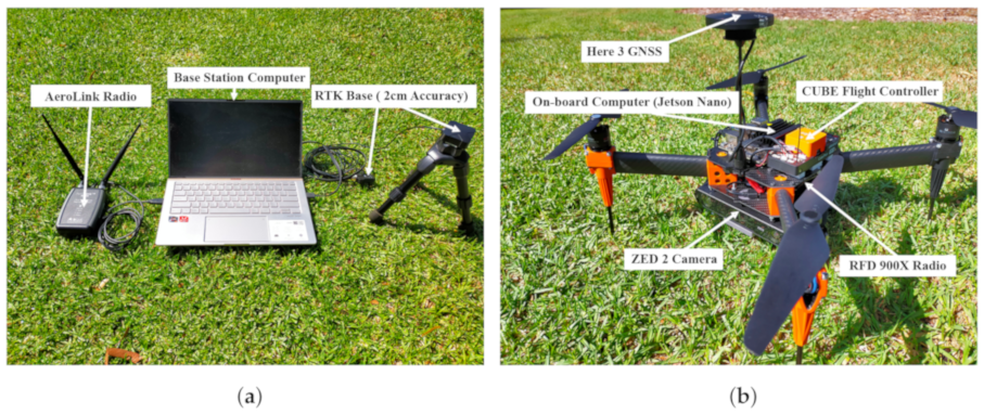
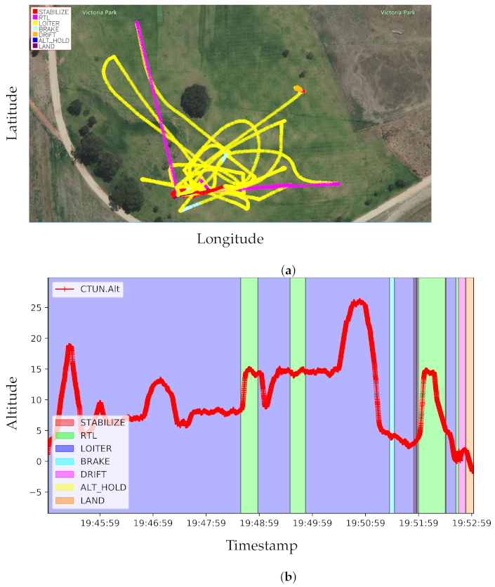
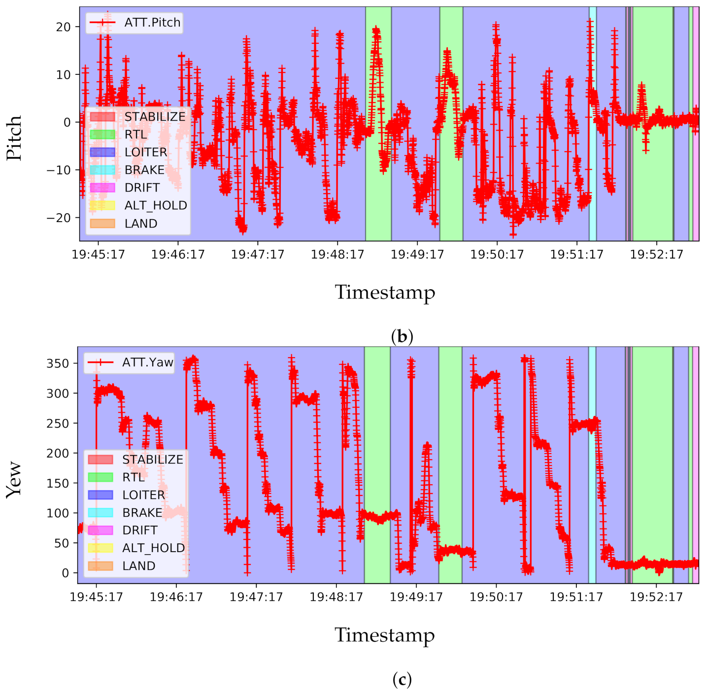
- A new benchmarking Micro Aerial Vehicle (MAV) dataset has been introduced for visual place recognition and V-SLAM evaluation.
2. Related Work
3. Proposed Method
3.1. Meaningful Feature Selection
3.2. Topological Database
3.3. Database Query and Geometrical Verification
3.3.1. Points Picking Policy
3.3.2. Computing Similar Triangle
4. Experimental Evaluation
4.1. Experimental Setup
4.2. Evaluation Metrics
4.3. Experimental Results
5. Conclusions
Author Contributions
Funding
Data Availability Statement
Conflicts of Interest
Abbreviations
| BoW | Bag-of-Words |
| CPU | Central Processing Unit |
| CNN | Convolutional Neural Network |
| DNN | Deep Neural Network |
| EKF | Extended Kalman Filter |
| GNSS | Global Navigation Satellite System |
| GPS | Global Positioning System |
| GPU | Graphics Processing Unit |
| IMU | Inertial Measurement Unit |
| i2i | Image-to-Image |
| LSTM | Long Short Term Memory |
| MAV | Micro Aerial Vehicle |
| PGO | Pose Graph Optimization |
| PnP | Perspective-n-Point |
| RTK | Real-Time Kinematic |
| SBC | Single Board Computer |
| SLAM | Simultaneous Localization and Mapping |
| UniSA | University of South Australia |
| UniSA-MLK | University of South Australia—Mawson Lakes |
| VPR | Visual Place Recognition |
| V-SLAM | Visual Simultaneous Localization and Mapping |
References
- Zeng, Z.; Zhang, J.; Wang, X.; Chen, Y.; Zhu, C. Place Recognition: An Overview of Vision Perspective. Appl. Sci. 2018, 8, 2257. [Google Scholar] [CrossRef]
- Bampis, L.; Amanatiadis, A.; Gasteratos, A. Encoding the description of image sequences: A two-layered pipeline for loop closure detection. In Proceedings of the IEEE/RSJ International Conference on Intelligent Robots and Systems (IROS), Daejeon, Republic of Korea, 9–14 October 2016; pp. 4530–4536. [Google Scholar]
- Kümmerle, R.; Grisetti, G.; Strasdat, H.; Konolige, K.; Burgard, W. g2o: A general framework for graph optimization. In Proceedings of the IEEE International Conference on Robotics and Automation, Shanghai, China, 9–13 May 2011; pp. 3607–3613. [Google Scholar]
- Williams, B.; Cummins, M.; Neira, J.; Newman, P.; Reid, I.; Tardós, J.D. A comparison of loop closing techniques in monocular SLAM. Robot. Auton. Syst. 2009, 57, 1188–1197. [Google Scholar] [CrossRef]
- Cummins, M.; Newman, P. FAB-MAP: Probabilistic localization and mapping in the space of appearance. Int. J. Robot. Res. 2008, 27, 647–665. [Google Scholar] [CrossRef]
- Chen, L.C.; Papandreou, G.; Kokkinos, I.; Murphy, K.; Yuille, A. DeepLab: Semantic Image Segmentation with Deep Convolutional Nets, Atrous Convolution, and Fully Connected CRFs. IEEE Trans. Pattern Anal. Mach. Intell. 2018, 40, 834–848. [Google Scholar] [CrossRef]
- Islam, R.; Habibullah, H. A Semantically Aware Place Recognition System for Loop Closure of a Visual SLAM System. In Proceedings of the 2021 4th International Conference on Mechatronics, Robotics and Automation (ICMRA), Zhanjiang, China, 22–24 October 2021; pp. 117–121. [Google Scholar]
- Lowry, S.; Sünderhauf, N.; Newman, P.; Leonard, J.J.; Cox, D.; Corke, P.; Milford, M.J. Visual Place Recognition: A Survey. IEEE Trans. Robot. 2016, 32, 1–19. [Google Scholar] [CrossRef]
- Torralba, A.; Murphy, K.P.; Freeman, W.T.; Rubin, M.A. Context-based vision system for place and object recognition. In Proceedings of the Ninth IEEE International Conference on Computer Vision, Nice, France, 13–16 October 2003; Volume 1, pp. 273–280. [Google Scholar]
- Nicosevici, T.; García, R. Automatic Visual Bag-of-Words for Online Robot Navigation and Mapping. IEEE Trans. Robot. 2012, 28, 886–898. [Google Scholar] [CrossRef]
- Lerma, C.D.C.; Gálvez-López, D.; Tardós, J.D.; Neira, J. Robust Place Recognition With Stereo Sequences. IEEE Trans. Robot. 2012, 28, 871–885. [Google Scholar]
- Nistér, D.; Stewénius, H. Scalable Recognition with a Vocabulary Tree. In Proceedings of the 2006 IEEE Computer Society Conference on Computer Vision and Pattern Recognition (CVPR’06), New York, NY, USA, 17–22 June 2006; Volume 2, pp. 2161–2168. [Google Scholar]
- Gálvez-López, D.; Tardós, J.D. Bags of Binary Words for Fast Place Recognition in Image Sequences. IEEE Trans. Robot. 2012, 28, 1188–1197. [Google Scholar] [CrossRef]
- Koniusz, P.; Yan, F.; Gosselin, P.H.; Mikolajczyk, K. Higher-Order Occurrence Pooling for Bags-of-Words: Visual Concept Detection. IEEE Trans. Pattern Anal. Mach. Intell. 2017, 39, 313–326. [Google Scholar] [CrossRef]
- Keetha, N.V.; Milford, M.; Garg, S. A Hierarchical Dual Model of Environment- and Place-Specific Utility for Visual Place Recognition. IEEE Robot. Autom. Lett. 2021, 6, 6969–6976. [Google Scholar] [CrossRef]
- Bhutta, M.U.M.; Sun, Y.; Lau, D.; Liu, M. Why-So-Deep: Towards Boosting Previously Trained Models for Visual Place Recognition. IEEE Robot. Autom. Lett. 2022, 7, 1824–1831. [Google Scholar] [CrossRef]
- Khaliq, A.; Milford, M.; Garg, S. MultiRes-NetVLAD: Augmenting Place Recognition Training with Low-Resolution Imagery. IEEE Robot. Autom. Lett. 2022, 7, 3882–3889. [Google Scholar] [CrossRef]
- Cai, K.; Wang, B.; Lu, C.X. AutoPlace: Robust Place Recognition with Single-chip Automotive Radar. In Proceedings of the 2022 International Conference on Robotics and Automation (ICRA), Philadelphia, PA, USA, 23–27 May 2022; pp. 2222–2228. [Google Scholar]
- Cai, Y.; Zhao, J.; Cui, J.; Zhang, F.; Ye, C.; Feng, T. Patch-NetVLAD+: Learned patch descriptor and weighted matching strategy for place recognition. In Proceedings of the 2022 IEEE International Conference on Multisensor Fusion and Integration for Intelligent Systems (MFI), Bedford, UK, 20–22 September 2022; pp. 1–8. [Google Scholar]
- Hausler, S.; Garg, S.; Xu, M.; Milford, M.; Fischer, T. Patch-NetVLAD: Multi-Scale Fusion of Locally-Global Descriptors for Place Recognition. In Proceedings of the 2021 IEEE/CVF Conference on Computer Vision and Pattern Recognition (CVPR), Nashville, TN, USA, 20–25 June 2021; pp. 14136–14147. [Google Scholar]
- Dietsche, A.; Ott, L.; Siegwart, R.Y.; Brockers, R. Visual Loop Closure Detection for a Future Mars Science Helicopter. IEEE Robot. Autom. Lett. 2022, 7, 12014–12021. [Google Scholar] [CrossRef]
- Xin, Z.; Cai, Y.; Lu, T.; Xing, X.; Cai, S.; Zhang, J.; Yang, Y.; Wang, Y. Localizing Discriminative Visual Landmarks for Place Recognition. In Proceedings of the 2019 International Conference on Robotics and Automation (ICRA), Montreal, QC, Canada, 20–24 May 2019; pp. 5979–5985. [Google Scholar]
- Schönberger, J.L.; Pollefeys, M.; Geiger, A.; Sattler, T. Semantic Visual Localization. In Proceedings of the IEEE/CVF Conference on Computer Vision and Pattern Recognition, Salt Lake City, UT, USA, 18–23 June 2018; pp. 6896–6906. [Google Scholar]
- Simonyan, K.; Zisserman, A. Very Deep Convolutional Networks for Large-Scale Image Recognition. arXiv 2015, arXiv:1409.1556. [Google Scholar]
- Masone, C.; Caputo, B. A Survey on Deep Visual Place Recognition. IEEE Access 2021, 9, 19516–19547. [Google Scholar] [CrossRef]
- Naseer, T.; Oliveira, G.L.; Brox, T.; Burgard, W. Semantics-aware visual localization under challenging perceptual conditions. In Proceedings of the IEEE International Conference on Robotics and Automation (ICRA), Singapore, 29 May–3 June 2017; pp. 2614–2620. [Google Scholar]
- Li, P.; Li, X.; Li, X.; Pan, H.; Khyam, M.O.; Noor-A-Rahim, M.; Ge, S.S. Place perception from the fusion of different image representation. Pattern Recognit. 2021, 110, 107680. [Google Scholar] [CrossRef]
- Mousavian, A.; Kosecka, J.; Lien, J.M. Semantically guided location recognition for outdoors scenes. In Proceedings of the IEEE International Conference on Robotics and Automation (ICRA), Seattle, WA, USA, 26–30 May 2015; pp. 4882–4889. [Google Scholar]
- Arandjelović, R.; Gronát, P.; Torii, A.; Pajdla, T.; Sivic, J. NetVLAD: CNN Architecture for Weakly Supervised Place Recognition. IEEE Trans. Pattern Anal. Mach. Intell. 2018, 40, 1437–1451. [Google Scholar] [CrossRef]
- Li, X.; Li, X.; Khyam, M.O.; Luo, C.; Tan, Y. Visual navigation method for indoor mobile robot based on extended BoW model. CAAI Trans. Intell. Technol. 2017, 2, 142–147. [Google Scholar] [CrossRef]
- Ali-bey, A.; Chaib-draa, B.; Giguère, P. GSV-Cities: Toward Appropriate Supervised Visual Place Recognition. Neurocomputing 2022, 513, 194–203. [Google Scholar] [CrossRef]
- Sünderhauf, N.; Dayoub, F.; Shirazi, S.A.; Upcroft, B.; Milford, M. On the performance of ConvNet features for place recognition. In Proceedings of the IEEE/RSJ International Conference on Intelligent Robots and Systems (IROS), Hamburg, Germany, 28 September–3 October 2015; pp. 4297–4304. [Google Scholar]
- Zhou, B.; Lapedriza, À.; Xiao, J.; Torralba, A.; Oliva, A. Learning Deep Features for Scene Recognition using Places Database. In Proceedings of the NIPS, Montreal, QC, Canada, 8–13 December 2014. [Google Scholar]
- Zaffar, M.; Ehsan, S.; Milford, M.; Flynn, D.; Mcdonald-Maier, K.D. VPR-Bench: An Open-Source Visual Place Recognition Evaluation Framework with Quantifiable Viewpoint and Appearance Change. Int. J. Comput. Vis. 2021, 129, 2136–2174. [Google Scholar] [CrossRef]
- Jiwei, N.; Feng, J.M.; Xue, D.; Feng, P.; Wei, L.; Jun, H.; Cheng, S. A Novel Image Descriptor with Aggregated Semantic Skeleton Representation for Long-term Visual Place Recognition. arXiv 2022, arXiv:abs/2202.03677. [Google Scholar]
- Razavian, A.S.; Azizpour, H.; Sullivan, J.; Carlsson, S. CNN Features Off-the-Shelf: An Astounding Baseline for Recognition. In Proceedings of the IEEE Conference on Computer Vision and Pattern Recognition Workshops, Columbus, OH, USA, 23–28 June 2014; pp. 512–519. [Google Scholar]
- Gong, Y.; Wang, L.; Guo, R.; Lazebnik, S. Multi-scale orderless pooling of deep convolutional activation features. In Proceedings of the 13th European Conference, Zurich, Switzerland, 6–12 September 2014; Springer: Cham, Switzerland, 2014; pp. 392–407. [Google Scholar]
- Liu, Y.; Guo, Y.; Wu, S.; Lew, M.S. Deepindex for accurate and efficient image retrieval. In Proceedings of the 5th ACM on International Conference on Multimedia Retrieval, Shanghai, China, 23–26 June 2015; pp. 43–50. [Google Scholar]
- Wan, J.; Wang, D.; Hoi, S.C.H.; Wu, P.; Zhu, J.; Zhang, Y.; Li, J. Deep learning for content-based image retrieval: A comprehensive study. In Proceedings of the ACM International Conference on Multimedia, Orlando, FL, USA, 3–7 November 2014; pp. 157–166. [Google Scholar]
- Gomez-Ojeda, R.; Lopez-Antequera, M.; Petkov, N.; Gonzalez-Jimenez, J. Training a convolutional neural network for appearance-invariant place recognition. arXiv 2015, arXiv:1505.07428. [Google Scholar]
- Brostow, G.J.; Fauqueur, J.; Cipolla, R. Semantic object classes in video: A high-definition ground truth database. Pattern Recognit. Lett. 2009, 30, 88–97. [Google Scholar] [CrossRef]
- Kendall, A.; Badrinarayanan, V.; Cipolla, R. Bayesian SegNet: Model Uncertainty in Deep Convolutional Encoder-Decoder Architectures for Scene Understanding. arXiv 2017, arXiv:1511.02680. [Google Scholar]
- LoweDavid, G. Distinctive Image Features from Scale-Invariant Keypoints. Int. J. Comput. Vis. 2004, 60, 91–110. [Google Scholar]
- Lepetit, V.; Moreno-Noguer, F.; Fua, P. EPnP: An Accurate O(n) Solution to the PnP Problem. Int. J. Comput. Vis. 2008, 81, 155–166. [Google Scholar] [CrossRef]
- Bonarini, A.; Burgard, W.; Fontana, G.; Matteucci, M.; Sorrenti, D.G.; Tardos, J.D. Rawseeds: Robotics advancement through web-publishing of sensorial and elaborated extensive data sets. In Proceedings of the 2006 IEEE/RSJ International Conference on Intelligent Robots and Systems (IROS), Beijing, China, 9–15 October 2006; Volume 6, p. 93. [Google Scholar]
- Smith, M.; Baldwin, I.; Churchill, W.; Paul, R.; Newman, P. The New College Vision and Laser Data Set. Int. J. Robot. Res. 2009, 28, 595–599. [Google Scholar] [CrossRef]
- Blanco, J.; Moreno, F.; González, J. A collection of outdoor robotic datasets with centimeter-accuracy ground truth. Auton. Robot. 2009, 27, 327–351. [Google Scholar] [CrossRef]
- Sarlin, P.E.; DeTone, D.; Malisiewicz, T.; Rabinovich, A. SuperGlue: Learning Feature Matching With Graph Neural Networks. In Proceedings of the IEEE/CVF Conference on Computer Vision and Pattern Recognition (CVPR), Seattle, WA, USA, 13–19 June 2020; pp. 4937–4946. [Google Scholar]
- Sarlin, P.E.; Cadena, C.; Siegwart, R.; Dymczyk, M. From Coarse to Fine: Robust Hierarchical Localization at Large Scale. In Proceedings of the IEEE/CVF Conference on Computer Vision and Pattern Recognition (CVPR), Long Beach, CA, USA, 15–20 June 2019; pp. 12708–12717. [Google Scholar]


| Dataset | Resolution | Network | Accuracy | Jetson Xavier |
|---|---|---|---|---|
| Cityscapes | 512 × 256 | fcn-resnet18 | 83.3% | 480 FPS |
| Cityscapes | 1024 × 521 | fcn-resnet18 | 87.3% | 176 FPS |
| DeepScene | 576 × 320 | fcn-resnet18 | 96.4% | 360 FPS |
| Pascal VOC | 512 × 400 | fcn-resnet18 | 64.0% | 340 FPS |
| Dataset | Description | Image Size |
|---|---|---|
| (px × px) | ||
| Outdoors, | ||
| New College [46] | Dynamic Objects, | 512 × 384 @ 20 Hz |
| Frontal Camera | ||
| Indoors, | ||
| Bicocca [45] | Static Objects, | 640 × 480 |
| Frontal Camera | ||
| Urban Area, | ||
| City Centre [5] | Dynamic Objects, | 640 × 480 |
| Lateral Camera | ||
| Outdoors, | ||
| Malaga [47] | Dynamic Objects, | 1024 × 768 |
| Lateral Camera | ||
| Outdoors, | ||
| Victoria Park, Adelaide, Australia [Ours] | Dynamic Objects, | 1024 × 720 @ 30 Hz |
| Frontal Stereo Camera |
| JETSON AGX XAVIER | ZED 2 CAMERA | ||
|---|---|---|---|
| GPU | 512-core Volta GPU with Tensor Cores | Depth FPS | Up to 100 Hz |
| CPU | 8-core ARM v8.2 64-bit CPU, 8 MB L2 + 4 MB L3 | Depth Range | 0.2–20 m (0.65 to 65 ft) |
| Memory | 32 GB 256-Bit LPDDR4× | 137 GB/s | Sensors | Accelerator, Gyroscope, Barometer, Magnetometer, Temperature Sensor |
| Storage | 32 GB eMMC 5.1 | Lens | Wide-angle with optically corrected distortion |
| DL Accelerator | (2×) NVDLA Engines | Field of View | 110° (H) × 70° (V) × 120° (D) max. |
| Vision Accelerator | 7-way VLIW Vision Processor | Aperture | ƒ/1.8 |
| Encoder/Decoder | (2×) 4Kp60 | HEVC/(2×) 4Kp60 | 12-Bit Support | Sensor Resolution | Dual 4M pixels sensors with 2-micron pixels |
| Dataset | Methods | Precision (%) | Recall (%) |
|---|---|---|---|
| New College | Proposed | 100 | 75.80 |
| Sarlin [49] | 100 | 62.25 | |
| DBoW2 [13] | 100 | 60.12 | |
| FAB-MAP [5] | 100 | 52.54 | |
| Malaga6L | Proposed | 100 | 77.45 |
| Sarlin [49] | 100 | 78.42 | |
| DBoW2 [13] | 100 | 72.56 | |
| FAB-MAP [5] | 100 | 65.87 | |
| Bicocca25b | Proposed | 100 | 85.32 |
| Sarlin [49] | 100 | 80.20 | |
| DBoW2 [13] | 100 | 56.52 | |
| FAB-MAP [5] | 100 | N/A | |
| City Center | Proposed | 100 | 65.45 |
| Sarlin [49] | 100 | 45.15 | |
| DBoW2 [13] | 100 | 32.73 | |
| FAB-MAP [5] | 100 | 36.64 | |
| Victoria Park | Proposed | 100 | 72.23 |
| Sarlin [49] | 100 | 53.50 | |
| DBoW2 [13] | 100 | 42.25 | |
| FAB-MAP [5] | 100 | 38.70 |
| Tasks | Execution Time (ms) | |||
|---|---|---|---|---|
| Mean | Std | Min | Max | |
| Attention Network | 2.85 | 0.45 | 1.52 | 5.65 |
| Feature Extraction | 10.81 | 6.44 | 7.00 | 56.00 |
| Bag of Words | 7.47 | 3.54 | 3.00 | 25.00 |
| Geometrical Verification | 2.50 | 2.41 | 1.48 | 10.50 |
| Total Time | 23.63 | 12.84 | 13.00 | 96.00 |
Publisher’s Note: MDPI stays neutral with regard to jurisdictional claims in published maps and institutional affiliations. |
© 2022 by the authors. Licensee MDPI, Basel, Switzerland. This article is an open access article distributed under the terms and conditions of the Creative Commons Attribution (CC BY) license (https://creativecommons.org/licenses/by/4.0/).
Share and Cite
Islam, R.; Habibullah, H. Place Recognition with Memorable and Stable Cues for Loop Closure of Visual SLAM Systems. Robotics 2022, 11, 142. https://doi.org/10.3390/robotics11060142
Islam R, Habibullah H. Place Recognition with Memorable and Stable Cues for Loop Closure of Visual SLAM Systems. Robotics. 2022; 11(6):142. https://doi.org/10.3390/robotics11060142
Chicago/Turabian StyleIslam, Rafiqul, and Habibullah Habibullah. 2022. "Place Recognition with Memorable and Stable Cues for Loop Closure of Visual SLAM Systems" Robotics 11, no. 6: 142. https://doi.org/10.3390/robotics11060142
APA StyleIslam, R., & Habibullah, H. (2022). Place Recognition with Memorable and Stable Cues for Loop Closure of Visual SLAM Systems. Robotics, 11(6), 142. https://doi.org/10.3390/robotics11060142