A Backstepping Approach to Nonlinear Model Predictive Horizon for Optimal Trajectory Planning

Abstract

This paper presents a novel trajectory planning approach for nonlinear dynamical systems; a multi-rotor drone, built on an optimization-based framework proposed by the authors named the Nonlinear Model Predictive Horizon. In the present work, this method is integrated with a Backstepping Control technique. The goal is to remove the non-convexity of the optimization problem in order to provide real-time computation of reference trajectories for the vehicle which respects its dynamics while avoiding sensed static and dynamic obstacles in the environment. Our method is applied to two models of multi-rotor drones to demonstrate its flexibility. Several simulation and hardware flight experiments are presented to validate the proposed design and demonstrate its performance improvement over earlier work.

1. Introduction

Planning collision-free trajectories for autonomous unmanned vehicles operating within unknown, dynamic, 3D, geometrically complex, and GPS-denied environments is a challenging and exciting research problem for both academia and industry. For agile drone systems, generating efficient trajectories in real-time requires using trajectory planning methods which respect the vehicle’s dynamics and input constraints as part of the prediction process. Researchers are now studying trajectory planning approaches which can take these considerations into account, for instance receding horizon-based methods [1,2,3].

Trajectory planning provides a parameterized path from a starting configuration to a terminal setpoint while avoiding obstacles. It is sometimes called motion planning and mistakenly referred to as path planning, since trajectory planning is a superset of path planning by generating reference kinematics over the entire path instead of geometric paths only [4]. Planning algorithms have received much attention from robotics researchers, where most of the published algorithms fall under one of the following categories: search-based, sampling-based, artificial potential field, artificial intelligence and optimization-based methods.

Search-based methods, a.k.a. grid-based methods, use search algorithms to find the best possible collision-free path in a discretized graph of grids. Some of the widely used graph search algorithms include Dijkstra algorithm [5], A* [6], Lifelong Planning A* (LPA*) [7], D* Lite [8], Anytime Repairing A* (ARA*) [9], and Hybrid-state A* [10]. The sampling-based approaches randomly sample a space of possible robot configurations distributed in space and use search algorithms to form a directed graph of collision-free motions. Probabilistic Road-Map (PRM) [11], Rapidly-Exploring Random Tree (RRT) [12], RRT*, and Rapidly-Exploring Random Graph (RRG) methods [13] are some examples of this thoroughly studied approach in the literature. The artificial potential field method developed in [14] plans a path to a goal that avoids collisions by assigning an attractive force to the desired goal and repulsive forces to obstacles [15]. A variety of artificial intelligence-based algorithms for path planning have been proposed in the literature, for instance, Artificial Neural Network (ANN) [16], Genetic Algorithm (GA) [17], Ant Colony Optimization (ACO) [18], Particle Swarm Optimization (PSO) [19], and Simulated Annealing (SA) [20] algorithms. Reference [21] presents a comprehensive review of artificial intelligence-based methods for path planning up to 2018. A recent line of research involves trajectory generation for flexible space robots based on deterministic artificial intelligence, which aims to use the dynamic equations of the system to autonomously determine an optimal reference trajectory (c.f. [22] and the references therein).

However, the above-mentioned motion planning algorithms have analytical and practical limitations, such as:

• Absence or limited consideration of the internal and external constraints imposed by the system and dynamic environment;
• Lack of repeatability in generating trajectories between a starting and ending configuration for a fixed initial vehicle state and environment scenario;
• Computational inefficiency in regenerating paths while moving between the start and terminal point;
• For some approaches, generating non-smooth paths that lead to jerky motions and create inefficiency in the vehicle’s power draw [23].

Recently, optimization-based motion planning methods have gained researchers’ attention due to their ability to resolve some or all of the above-mentioned limitations. The best-known optimization-based methods for motion planning are Covariant Hamiltonian Optimization for Motion Planning (CHOMP) [24] and Stochastic Trajectory Optimization for Motion Planning (STOMP) [25]. The former uses gradient-based optimization while the latter uses stochastic optimization, and both produce collision-free trajectories that satisfy given constraints, but are computationally expensive. In addition, CHOMP is prone to getting trapped in local minima, where it returns infeasible or sub-optimal solutions. A very recent publication on optimization-based trajectory generation is [26], which uses Pontryagin’s maximum principle to efficiently generate slew trajectories for a spacecraft.

Our proposed approach, called the Nonlinear Model Predictive Horizon (NMPH) [27], uses optimization for planning smooth, optimal, consistent, and computationally efficient trajectories which respect the internal and external constraints of the vehicle. This approach compensates for the nonlinearities of the trajectory planning dynamics and hence reduces or removes the non-convexity of the optimization problem. This is performed by combining the nonlinear plant model with the Backstepping Control (BSC) method within the optimization problem. It also accounts for static and moving obstacles as constraints in the optimization problem.

In ref. [27], we proposed an NMPH formulation which used Feedback Linearization (FBL) within its dynamics to compensate for nonlinearities. In that work, the state augmentation process required to make the system state feedback linearizable created numerical difficulties due to the need to obtain the second-order time derivative of the total thrust of the drone. This difficulty with using the FBL design steered us to find an alternative feedback design methodology to be used within the NMPH design, namely BSC. This new NMPH-BSC formulation compensates for the system nonlinearities and guarantees global asymptotic stability of the closed-loop system within the optimization problem used to predict the reference trajectories for the drone vehicle.

The backstepping control algorithm was originally developed by [28] to design adaptive controllers for a special class of nonlinear dynamical systems. Backstepping is a recursive Lyapunov-based design technique applied to a nonlinear strict-feedback system with a series of cascaded subsystems, in which the choice of the Lyapunov functions for the subsystems guarantees the global asymptotic stability of the overall controlled system [29].

One of the most important advantages of the BSC method is the systematic procedure that the designer can follow to construct a feedback control law based on an appropriate choice of Lyapunov functions [30]. This step-by-step procedure uses the system’s dynamics model, which accounts for the system nonlinearities.

The flexibility of the BSC methodology and its ability to guarantee global asymptotic stability [31,32] make it an excellent candidate to be used inside the NMPH approach, as this integration compensates for the drone’s nonlinearities and leads to a less non-convex optimization problem.

To demonstrate the versatility of our NMPH-BSC approach over the earlier NMPH-FBL [27], a more detailed model of the drone vehicle dynamics, which includes linear and angular velocity drag forces and rotor gyroscopic effects, is employed. The optimization problem is also used to predict both the reference trajectory as well as its rates of change, which provides higher-quality tracking performance.

The research contributions of this paper are:

• Implementing the BSC method within NMPH to compensate for nonlinearities in order to reduce the non-convexity of the trajectory generation optimization problem;
• Demonstrating the versatility of the NMPH-BSC approach by using both a simplified and a higher-fidelity dynamics model of the drone;
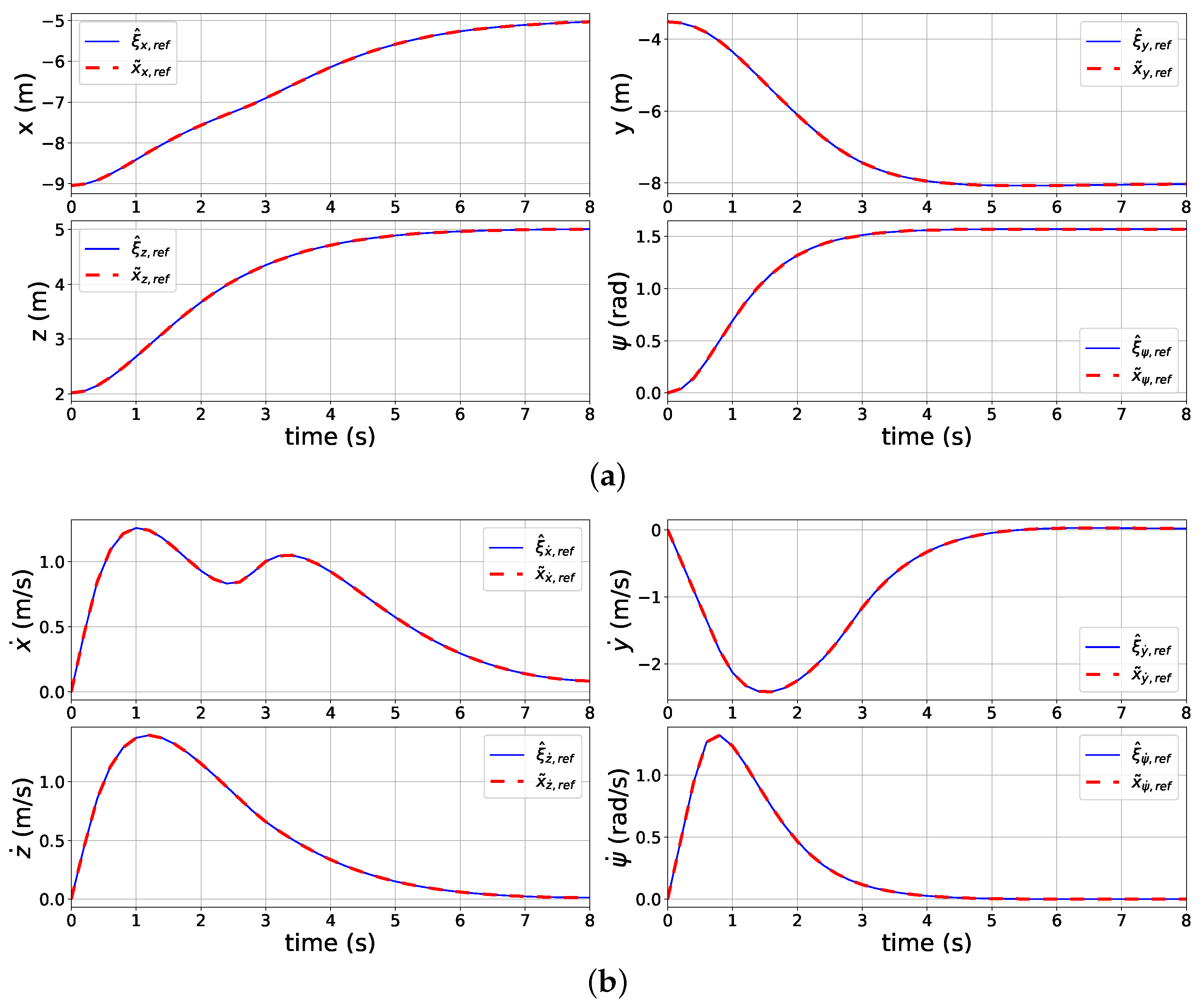
• Using the NMPH optimization problem to predict both the reference trajectory as well as its rates of change for the onboard flight trajectory controller;
• Validating and evaluating the performance of the proposed approach in both simulation and hardware drone flight experiments.

The remainder of this paper is arranged as follows: the design of the NMPH-BSC for two variants of drone dynamics models is presented in Section 2. Section 3 evaluates the proposed designs in simulation and hardware flight tests. Section 4 summarizes the paper and proposes future work.

2. Problem Formulation

The Nonlinear Model Predictive Horizon (NMPH) is a recent approach to path planning proposed by the authors in [27]. In simple terms, NMPH integrates a linearizing feedback law to reduce the non-convexity of the optimization problem handled by a Nonlinear Model Predictive Control (NMPC) algorithm. NMPH generates optimal reference trajectories for the closed-loop system which steers an aerial drone’s 3D position, heading angle, and their rates of change. The original NMPH [27] relied on state feedback linearization [33], which required the addition of integral states to satisfy the conditions of the method, translating to the need for numerical differentiation of measured outputs. In the present work, we replace feedback linearization with Backstepping Control (BSC) [28] to compensate for the system’s nonlinearities. The recursive structure of BSC provides stable response of a dynamic system and makes it more robust to parameter uncertainties.

In this section, an overview of the NMPH framework is presented, both high-fidelity and simplified drone dynamics models are presented, and finally a backstepping design for each model is derived and integrated into the NMPH.

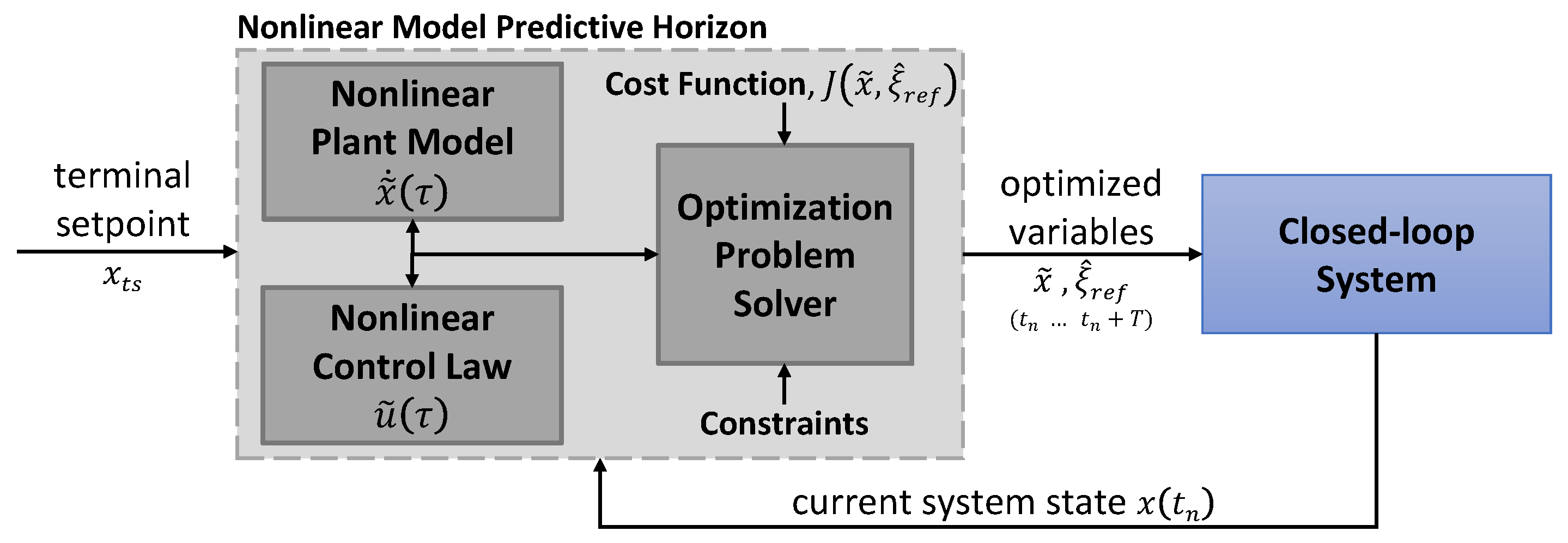
2.1. Nonlinear Model Predictive Horizon

NMPH is an optimization-based method whose objective is to generate optimal reference trajectories for closed-loop nonlinear systems. The optimization problem of NMPH considers the nonlinear plant model, nonlinear control law, and user-specified constraints to continuously solve for reference trajectories which are fed to the closed-loop system and which respect its dynamics. An overview of the NMPH architecture is shown in Figure 1.

Embedding the nonlinear control law in the optimization problem is performed to decrease the nonlinearity of the closed-loop system dynamics. Consequently, this will reduce the non-convexity of the optimization problem and enhance convergence and computational time of the solution, enabling real-time trajectory generation for purposes such as motion planning and environmental exploration.

For the closed-loop system, which is depicted by a blue box in Figure 1, assume that a nonlinear plant is controlled by a nonlinear feedback law as follows:

$$\begin{array}{cc}\hfill \dot{x}& =f\left(x,u\right)\hfill \end{array}$$

(1a)

$$\begin{array}{cc}\hfill \xi & =h\left(x\right)\hfill \end{array}$$

(1b)

$$\begin{array}{cc}\hfill u& =g(x,{\xi }_{{}_{ref}}),\hfill \end{array}$$

(1c)

where $x\in X\subseteq {\mathbb{R}}^{n_x}$, $u\in U\subseteq {\mathbb{R}}^{n_u}$, and $\xi \in \Xi \subseteq {\mathbb{R}}^{n_{\xi }}$ are the system states, inputs, and outputs, respectively. The system outputs considered in this work are the vehicle’s 3D position and heading angle and their rates, such that $\Xi \subseteq X$. The reference trajectory ${\xi }_{{}_{ref}}\in \Xi$ is generated by our proposed algorithm, as will be presented below in (2). The system dynamics are represented by a smooth map $f:X\times U\to X$, while the feedback control law is the smooth map $g:X\times \Xi \to U$ which makes the system output to follow a reference trajectory ${\xi }_{{}_{ref}}$. In this work the control law is designed using the Backstepping Control technique.

For the NMPH, which is represented by the gray box in Figure 1, a copy of (1) plus assigned constraints are used in the optimization problem to compute two predictions over a finite time horizon, from the current state x to a terminal stabilization setpoint $x_{{}_{ss}}$. The first prediction is the predicted system state trajectory $\tilde{x}$, which includes the predicted output trajectory $\tilde{\xi }$ as a subset. The second one is the estimated reference trajectory ${\widehat{\xi }}_{{}_{ref}}$, which is used as a (continuously updated) reference trajectory for the actual closed-loop system.

The online NMPH optimization problem for a stabilization setpoint $x_{{}_{ss}}$ is shown in Equation (2) [34]. Let $t_n$, $n=0,1,2,\cdots$ represent successive sampling times. At every sampling time, the optimization problem solves for $\tilde{x}$ and ${\widehat{\xi }}_{{}_{ref}}$ as long as $\parallel x_{{}_{ss}}-x\left(t_n\right)\parallel \ge \Delta$:

$$\begin{array}{cc}\hfill & \underset{\tilde{x},{\widehat{\xi }}_{{}_{ref}}}{min}\left(J\left(\tilde{x},{\widehat{\xi }}_{{}_{ref}}\right)=E\left(\tilde{x}\left(t_n+T\right)\right)+{\int }_{t_n}^{t_n+T}L\left(\tilde{x}\left(\tau \right),{\widehat{\xi }}_{{}_{ref}}\left(\tau \right)\right)d\tau \right)\hfill \end{array}$$

(2)

$$\begin{array}{cccc}\hfill \mathrm{subject}\mathrm{to}& \tilde{x}\left(t_n\right)=x\left(t_n\right),\hfill & \hfill & \hfill \end{array}$$

(2a)

$$\begin{array}{cccc}\hfill & \dot{\tilde{x}}\left(\tau \right)=f\left(\tilde{x}\left(\tau \right),\tilde{u}\left(\tau \right)\right),\hfill & \hfill & \hfill \end{array}$$

(2b)

$$\begin{array}{cccc}\hfill & \tilde{u}\left(\tau \right)=g\left(\tilde{x}\left(\tau \right),{\widehat{\xi }}_{{}_{ref}}\left(\tau \right)\right),\hfill & \hfill & \hfill \end{array}$$

(2c)

$$\begin{array}{cccc}\hfill & \tilde{x}\left(\tau \right)\in \mathcal{X},\tilde{u}\left(\tau \right)\in \mathcal{U},{\widehat{\xi }}_{{}_{ref}}\left(\tau \right)\in \mathcal{Z},\hfill & \hfill & \hfill \end{array}$$

(2d)

$$\begin{array}{cc}\hfill & {\mathcal{O}}_i\left(\tilde{x}\right)\le 0,i=1,2,\dots ,p,\hfill \end{array}$$

(2e)

$$\begin{array}{cc}\hfill \mathrm{for}& \tau \in [t_n,t_n+T].\hfill \end{array}$$

The stage L and terminal cost E functions in (2) can be selected as the terms (3a,b), which allows the use of the Gauss–Newton method for quickly finding a good approximation of the Hessian matrix within the optimization problem:

$$\begin{array}{cc}\hfill L\left(\tilde{x}\left(\tau \right),{\widehat{\xi }}_{{}_{ref}}\left(\tau \right)\right)& =\parallel \tilde{x}\left(\tau \right)-x_{{}_{ss}}{\parallel }_{W_x}^2+{\parallel \tilde{\xi }\left(\tau \right)-{\widehat{\xi }}_{{}_{ref}}\left(\tau \right)\parallel }_{W_{\xi }}^2\hfill \end{array}$$

(3a)

$$\begin{array}{cc}\hfill E\left(\tilde{x}\left(t_n+T\right)\right)& =\parallel \tilde{x}\left(t_n+T\right)-x_{{}_{ss}}{\parallel }_{W_T}^2,\hfill \end{array}$$

(3b)

where the constraint sets for the state, control and output trajectory are $\mathcal{X}\subseteq X$, $\mathcal{U}\subseteq U$, and $\mathcal{Z}\subseteq X$, respectively. A total of p static and dynamic obstacles within the environment are represented by the inequality constraint ${\mathcal{O}}_i\left(\tilde{x}\right)\le 0$ in (2e). The deviation between the predicted system state trajectory $\tilde{x}$ and the stabilization setpoint $x_{{}_{ss}}$ and between the predicted output trajectory $\tilde{\xi }$ and the estimated reference trajectory ${\widehat{\xi }}_{{}_{ref}}$ are penalized within the stage cost function L (3a) by the weighting matrices $W_x\in {\mathbb{R}}^{n_x\times n_x}$ and $W_{\xi }\in {\mathbb{R}}^{n_{\xi }\times n_{\xi }}$, respectively. The terminal cost function E (3b), which represents the cost of steady-state error, penalizes the deviation between the end value of the system state prediction $\tilde{x}\left(t_n+T\right)$ and the terminal setpoint $x_{{}_{ss}}$ by the weighting matrix $W_T$.

In words, the optimization process (2) runs as follows:

(1)

Measure or estimate the current state $x\left(t_n\right)$ of the actual closed-loop system;

(2)

Predict $\tilde{x}$ and ${\widehat{\xi }}_{{}_{ref}}$ by minimizing the cost function $J\left(\tilde{x},{\widehat{\xi }}_{{}_{ref}}\right)$ over the prediction horizon $[t_n,t_n+T]$ subject to the system dynamics (2b), control law (2c), and assigned constraints (2e);

(3)

Use the estimated reference trajectory ${\widehat{\xi }}_{{}_{ref}}$ (or the predicted output trajectory $\tilde{\xi }$, as both converge to each other) as the reference trajectory of the actual closed-loop system;

(4)

Repeat Steps 1–3 until the drone vehicle approaches the terminal setpoint $x_{{}_{ss}}$ or the optimization problem produces an infeasible solution.

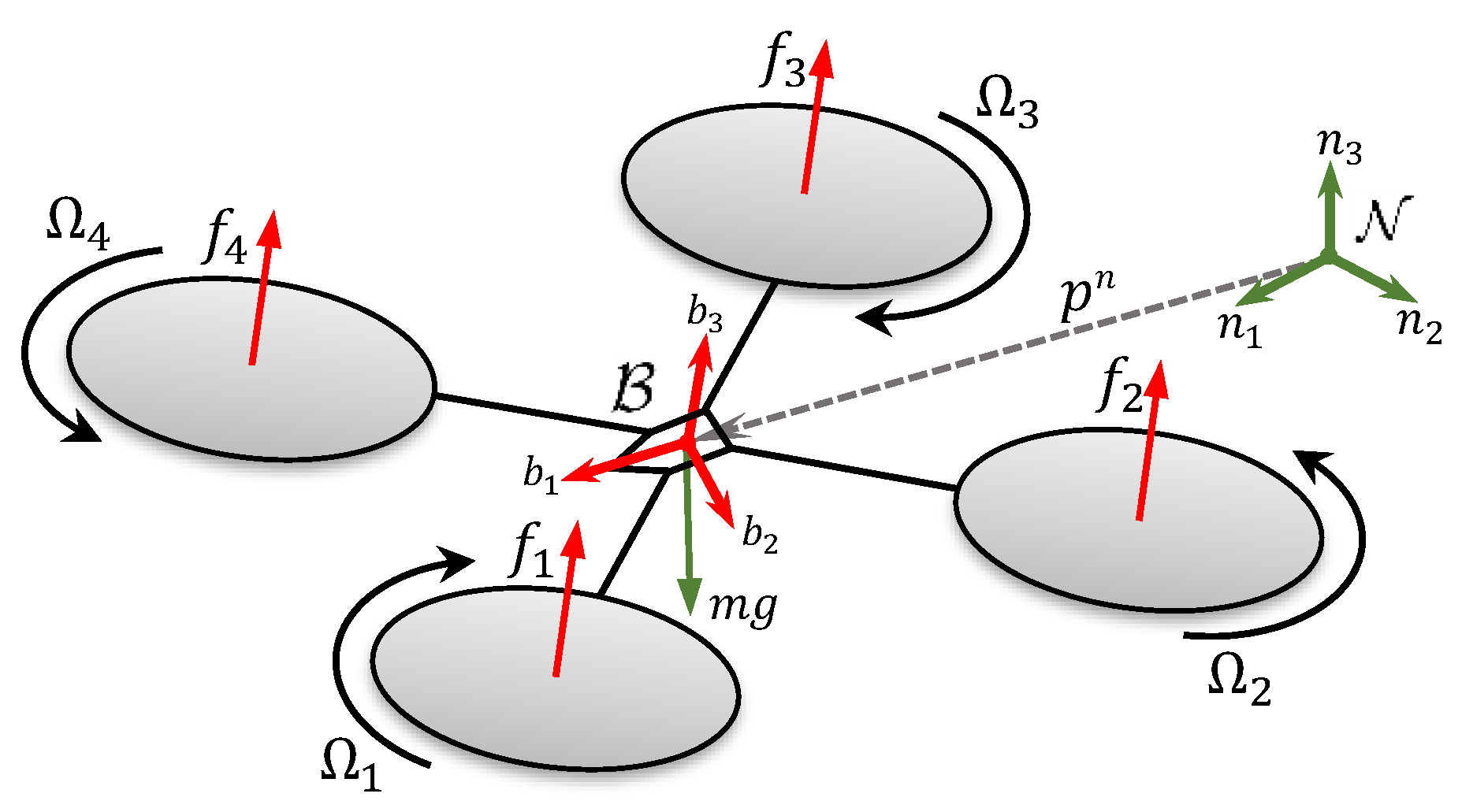
A comprehensive study about NMPH, including discrete-time representation, use of constraints, and software implementation of the optimization problem can be found in our recent work [27].

2.2. Drone Dynamics

The dynamics of a multi-rotor drone vehicle can be modeled using the Newton–Euler equations [35], governing six degrees of freedom rigid-body motion, augmented with force and torque generation models of the individual rotors. The model can either assume static hover conditions for simplicity, or include linear and angular velocity drag forces and rotor gyroscopic effects to yield a more complicated but higher-fidelity model.

To model rigid-body dynamics, two reference frames are used: a stationary ground-fixed navigation frame $\mathcal{N}$, and a moving body-fixed frame $\mathcal{B}$. The origin of the latter is placed at the drone’s center of gravity, as shown in Figure 2. The frame bases follow the East, North, and Up (ENU) convention, with orthonormal basis vectors $\{n_1,n_2,n_3\}$ and $\{b_1,b_2,b_3\}$ for the navigation and body frames, respectively.

Rigid-body pose in space can be described as a member of the Special Euclidean group $\mathrm{SE}\left(3\right)=\mathrm{SO}\left(3\right)\times {\mathbb{R}}^3$, the product space of the orientation and position $\left(R_{{}_{nb}},p^n\right)$ where $R_{{}_{nb}}\in \mathrm{SO}\left(3\right)$ is the rotation matrix of the body frame with respect to the navigation frame, $p^n={\left[xyz\right]}^T\in {\mathbb{R}}^3$ is the position vector of the vehicle’s body frame with respect to the navigation frame, and $\mathrm{SO}\left(3\right)$ is the Special Orthogonal group defined as $\mathrm{SO}\left(3\right)=\{R\in {\mathbb{R}}^{3\times 3}|R{R}^T=R^{T}R=I,det\left(R\right)=+1\}$. The roll-pitch-yaw Euler angles $\eta ={\left[\varphi \theta \psi \right]}^T$ are employed to parametrize the rotation matrix as:

$$R_{{}_{nb}}=\left[\begin{array}{ccc}{c}_{\theta }{c}_{\psi }& s_{\varphi }{s}_{\theta }{c}_{\psi }-c_{\varphi }{s}_{\psi }& c_{\varphi }{s}_{\theta }{c}_{\psi }+s_{\varphi }{s}_{\psi }\\ c_{\theta }{s}_{\psi }& s_{\varphi }{s}_{\theta }{s}_{\psi }+c_{\varphi }{c}_{\psi }& c_{\varphi }{s}_{\theta }{s}_{\psi }-s_{\varphi }{c}_{\psi }\\ -s_{\theta }& s_{\varphi }{c}_{\theta }& c_{\varphi }{c}_{\theta }\end{array}\right]$$

(4)

where $s_{(·)}=sin(·)$ and $c_{(·)}=cos(·)$. Similarly, $t_{(·)}=tan(·)$ which will be seen later.

Remark 1.

The Euler angle parameterization exhibits singularities at $\theta =\pi /2+k\pi$, $k\in \mathbb{Z}$. One solution is to maintain $-\pi /2<\theta <\pi /2$ by adding constraints within the NMPH optimization problem under (2d).

Conversion between translational and rotational velocity vectors can be performed using the transformations [36]:

$$\begin{array}{cc}\hfill {\dot{p}}^n& =v^n=R_{{}_{nb}}{v}^b\hfill \end{array}$$

(5a)

$$\begin{array}{cc}\hfill {\omega }^b& =W\dot{\eta },\hfill \end{array}$$

(5b)

where $v^n,v^b\in {\mathbb{R}}^3$ are the translational velocity vectors in frame $\mathcal{N}$ and $\mathcal{B}$ coordinates, respectively, $\dot{\eta }={\left[\dot{\varphi }\dot{\theta }\dot{\psi }\right]}^T$ is the vector of Euler angle rates, and ${\omega }^b\in {\mathbb{R}}^3$ is the angular velocity vector in frame $\mathcal{B}$ coordinates. The rotational velocity transformation matrix W is given by:

$$W=\left[\begin{array}{ccc}1& 0& -s_{\theta }\\ 0& c_{\varphi }& s_{\varphi }{c}_{\theta }\\ 0& -s_{\varphi }& c_{\varphi }{c}_{\theta }.\end{array}\right]$$

(6)

The time derivative of the rotation matrix is ${\dot{R}}_{{}_{nb}}=R_{{}_{nb}}\mathcal{S}\left({\omega }^b\right)$, where $\mathcal{S}(·):{\mathbb{R}}^3\to \mathrm{so}\left(3\right)$ maps a vector to a skew-symmetric matrix such that $\mathcal{S}\left(a\right)b=a\times b$ for $a,b\in {\mathbb{R}}^3$. Taking the time derivatives of (5a,b),

$$\begin{array}{cc}\hfill {\dot{v}}^n& =R_{{}_{nb}}{\dot{v}}^b+R_{{}_{nb}}\mathcal{S}\left({\omega }^b\right)v^b=R_{{}_{nb}}\left({\dot{v}}^b+{\omega }^b\times v^b\right)\hfill \end{array}$$

(7a)

$$\begin{array}{cc}\hfill {\dot{\omega }}^b& =\dot{W}\dot{\eta }+W\ddot{\eta },\hfill \end{array}$$

(7b)

where $\dot{W}=\dot{\varphi }(\partial W/\partial \varphi )+\dot{\theta }(\partial W/\partial \theta )$.

The Newton–Euler equations for a multi-rotor drone read [36]

$$\begin{array}{cc}\hfill m{\dot{v}}^b+{\omega }^b\times m{v}^b& =\overline{u}-K_t{v}^b-m{R}_{{}_{nb}}^T\overline{g}\hfill \end{array}$$

(8a)

$$\begin{array}{cc}\hfill J{\dot{\omega }}^b+{\omega }^b\times J{\omega }^b& =\overline{\tau }-K_r{\omega }^b-\sum _{i=1}^4\left(\mathcal{S}\left({\omega }^b\right)J_r{q}_i\right),\hfill \end{array}$$

(8b)

where m is the drone’s mass, $\overline{u}={\left[00u\right]}^T$ is the thrust vector with $u={\sum }_{i=1}^4{f}_i$ the total thrust generated in the direction of $b_3$, $\overline{\tau }={\left[{\tau }^{b_1}{\tau }^{b_2}{\tau }^{b_3}\right]}^T$ is the vector of torques about the $b_1$, $b_2$ and $b_3$ frame axes, $\overline{g}={\left[00g\right]}^T$ is the gravitational acceleration vector where $g=9.81{\mathrm{m}/\mathrm{s}}^2$, $J=\mathrm{diag}(J_x,J_y,J_z)$ is the drone’s mass moment of inertia matrix which is assumed to be diagonal, the scalar $J_r$ is the rotor’s inertia, $q_i={\left[00{(-1)}^{i+1}{\omega }_i\right]}^T$ where ${\omega }_i$ is the angular speed of the ith propeller, and $K_t=\mathrm{diag}(k_{t1},k_{t2},k_{t3})$, $K_r=\mathrm{diag}(k_{r1},k_{r2},k_{r3})$ represent the translational and rotational drag coefficient matrices of the drone, respectively.

To express the drone’s dynamics with respect to the navigation frame, Equation (8) are combined with (5) and (7) to yield:

$$\begin{array}{cc}\hfill m{R}_{{}_{nb}}^T{\dot{v}}^n& =\overline{u}-K_t{R}_{{}_{nb}}^T{v}^n-m{R}_{{}_{nb}}^T\overline{g}\hfill \end{array}$$

(9a)

$$\begin{array}{cc}\hfill JW\ddot{\eta }+J\dot{W}\dot{\eta }+\mathcal{S}\left(W\dot{\eta }\right)JW\dot{\eta }& =\overline{\tau }-K_{r}W\dot{\eta }-\mathcal{S}\left(W\dot{\eta }\right)\sum _{i=1}^4{J}_r{q}_i.\hfill \end{array}$$

(9b)

This leads to:

$$\begin{array}{cc}\hfill {\dot{v}}^n& =-\frac{1}{m}{R}_{{}_{nb}}{K}_t{R}_{{}_{nb}}^T{v}^n-\overline{g}+\frac{1}{m}{R}_{{}_{nb}}\overline{u}\hfill \end{array}$$

(10a)

$$\begin{array}{cc}\hfill \ddot{\eta }& =-{\left(JW\right)}^{-1}(J\dot{W}\dot{\eta }+K_{r}W\dot{\eta }+\mathcal{S}(W\dot{\eta })(JW\dot{\eta }+\sum _{i=1}^4{J}_r{q}_i)-\overline{\tau }).\hfill \end{array}$$

(10b)

Remark 2.

Each multi-rotor configuration (quadrotor, hexarotor, octorotor, and so on) has a different expression for the net body-frame thrust and torque vectors $\overline{u}$ and $\overline{\tau }$. These expressions are algebraic and can be readily calculated. The dynamics presented in (10) thus model any multi-rotor drone as long as the correct $\overline{u}$ and $\overline{\tau }$ expressions are used.

The development of the proposed NMPH with a backstepping control design will be based on the dynamics model presented in (10). We will also present a design based on a simplified version of (10) to illustrate the ease of adapting the proposed approach to different model representations. This is in contrast to the formulation of NMPH with feedback linearization presented in our recent work [27] where this adaptation requires a fundamental re-derivation of the expressions involved.

In the simplified version of (10), body and propeller gyroscopic effects are dropped from the model, and the translational and rotational drags are neglected as well. The simplified model can then be written as:

$$\left[\begin{array}{c}\dot{\varphi }\\ \dot{\theta }\\ \dot{\psi }\\ \dot{x}\\ \dot{y}\\ \dot{z}\end{array}\right]=\left[\begin{array}{c}\frac{J_y-J_z}{J_x}\dot{\theta }\dot{\psi }+\frac{1}{J_x}{\tau }^{b_1}\\ \frac{J_z-J_x}{J_y}\dot{\varphi }\dot{\psi }+\frac{1}{J_y}{\tau }^{b_2}\\ \frac{J_x-J_y}{J_z}\dot{\varphi }\dot{\theta }+\frac{1}{J_z}{\tau }^{b_3}\\ (c_{\varphi }{s}_{\theta }{c}_{\psi }+s_{\varphi }{s}_{\psi })\frac{u}{m}\\ (c_{\varphi }{s}_{\theta }{s}_{\psi }-s_{\varphi }{c}_{\psi })\frac{u}{m}\\ -g+\left(c_{\varphi }{c}_{\theta }\right)\frac{u}{m}\end{array}\right].$$

(11)

2.3. Backstepping Control Design

Because a drone’s dynamics are nonlinear, solving the NMPC optimization problem is challenging because of its non-convexity. Introducing backstepping control into the optimization problem (within the framework of NMPH) will either remove or reduce the nonlinearity of the overall system, and consequently the non-convexity of the optimization problem. This will make it possible to find an optimal solution more quickly.

In this section, a backstepping control law is derived for the drone dynamics, which will be used within the NMPH framework to enhance the performance of the reference trajectory prediction. To demonstrate the versatility of this methodology, both the simplified (11) and high-fidelity (10) models of the drone dynamics will be considered.

Our backstepping control design consists of a coupling of inner and outer control loops [37]. The inner loop controls the rotational dynamics of the drone and tracks desired values provided by the outer loop, which controls the translational dynamics. In the literature, many studies of backstepping control applied to multi-rotor drones considered applying the design steps to each system output separately [36,38,39,40], but in our work the method is first applied to the rotational dynamics subsystem by itself, then to the translational dynamics subsystem. This approach will facilitate the integration of BSC within the NMPH framework as discussed later in Section 2.4.

First, recall the terms:

$$\eta ={\left[\varphi \theta \psi \right]}^T,\dot{\eta }={\left[\dot{\varphi }\dot{\theta }\dot{\psi }\right]}^T,{\eta }_{{}_d}={\left[{\varphi }_d{\theta }_d{\psi }_d\right]}^T,$$

(12)

where ${\eta }_{{}_d}\in {\mathbb{R}}^3$ are the desired Euler angles, to be provided by the outer loop design. Now, define the tracking error vector ${\delta }_1\in {\mathbb{R}}^3$ as:

$${\delta }_1={\eta }_{{}_d}-\eta ,$$

(13)

and choose a positive semi-definite Lyapunov function candidate $V_1\ge 0\in \mathbb{R}$, such that

$$V_1=\frac{1}{2}{\delta }_1^T{\delta }_1.$$

(14)

The time derivative of (14) is:

$${\dot{V}}_1={\delta }_1^T{\dot{\delta }}_1={\delta }_1^T({\dot{\eta }}_{{}_d}-\dot{\eta }).$$

(15)

Next, define the virtual tracking error rate ${\delta }_2\in {\mathbb{R}}^3$ and the first virtual control $v_1={\left[v_{\varphi }{v}_{\theta }{v}_{\psi }\right]}^T\in {\mathbb{R}}^3$ as:

$$\begin{array}{ccc}\hfill {\delta }_2& =& v_1-\dot{\eta }\hfill \end{array}$$

(16)

$$\begin{array}{ccc}\hfill v_1& =& {\dot{\eta }}_{{}_d}+{\Lambda }_1{\delta }_1,\hfill \end{array}$$

(17)

where ${\Lambda }_1=\mathrm{diag}({\lambda }_1,{\lambda }_2,{\lambda }_3)\in {\mathbb{R}}^{3\times 3}$ is a diagonal gain matrix that contains positive entries such that ${\Lambda }_1$ is positive definite or ${\Lambda }_1>0$. Using (16) and (17), the derivative of the Lyapunov function candidate (15) can be written as:

$${\dot{V}}_1={\delta }_1^T(v_1-{\Lambda }_1{\delta }_1-\dot{\eta })={\delta }_1^T({\delta }_2-{\Lambda }_1{\delta }_1)={\delta }_1^T{\delta }_2-{\delta }_1^T{\Lambda }_1{\delta }_1,$$

(18)

which by inspection may or may not be negative semi-definite. Therefore, a recursive step must be performed. Note that the time derivatives of (13) and (16) are:

$$\begin{array}{ccc}\hfill {\dot{\delta }}_1& =& {\dot{\eta }}_d-\dot{\eta }=v_1-{\Lambda }_1{\delta }_1+{\delta }_2-v_1=-{\Lambda }_1{\delta }_1+{\delta }_2\hfill \end{array}$$

(19)

$$\begin{array}{ccc}\hfill {\dot{\delta }}_2& =& {\dot{v}}_1-\ddot{\eta }={\ddot{\eta }}_{{}_d}+{\Lambda }_1{\dot{\delta }}_1-\ddot{\eta }.\hfill \end{array}$$

(20)

Now define the new positive semi-definite Lyapunov function candidate $V_2\ge 0\in \mathbb{R}$ as:

$$V_2=\frac{1}{2}{\delta }_1^T{\delta }_1+\frac{1}{2}{\delta }_2^T{\delta }_2,$$

(21)

such that

$$\begin{array}{cc}\hfill {\dot{V}}_2& ={\delta }_1^T{\dot{\delta }}_1+{\delta }_2^T{\dot{\delta }}_2\hfill \\ \hfill & =-{\delta }_1^T{\Lambda }_1{\delta }_1+{\delta }_1^T{\delta }_2+{\delta }_2^T\left({\ddot{\eta }}_{{}_d}+{\Lambda }_1(-{\Lambda }_1{\delta }_1+{\delta }_2)-\ddot{\eta }\right)\hfill \\ \hfill & =-{\delta }_1^T{\Lambda }_1{\delta }_1+{\delta }_2^T\left({\delta }_1+{\ddot{\eta }}_{{}_d}-{\Lambda }_1^2{\delta }_1+{\Lambda }_1{\delta }_2-\ddot{\eta }\right),\hfill \end{array}$$

(22)

where ${\delta }_1^T{\delta }_2={\delta }_2^T{\delta }_1$. To stabilize the tracking errors ${\delta }_1$ and ${\delta }_2$, the backstepping control formulation will introduce a second virtual control $v_2\in {\mathbb{R}}^3$. We will define $v_2$ based on the system dynamics, and then recursively design it within the backstepping control structure.

As mentioned in Section 2.2, we will apply the backstepping technique to both the full and simplified system dynamics presented in (10) and (11), respectively. For the full model, the attitude dynamics in (10b) can be written as:

$$\ddot{\eta }={\overline{f}}_1\left(x\right)+{\overline{g}}_1(x,\overline{\tau }),$$

(23)

where

$$\begin{array}{ccc}\hfill {\overline{f}}_1\left(x\right)& =& -{(JW)}^{-1}(J\dot{W}\dot{\eta }+K_{r}W\dot{\eta }+\mathcal{S}\left(W\dot{\eta }\right)(JW\dot{\eta }+\sum _{i=1}^4{J}_r{q}_i))\hfill \end{array}$$

(24)

$$\begin{array}{ccc}\hfill {\overline{g}}_1(x,\overline{\tau })& =& {\left(JW\right)}^{-1}\overline{\tau }=\left[\begin{array}{c}\frac{1}{J_x}{\tau }^{b_1}+\frac{1}{J_y}{s}_{\varphi }{t}_{\theta }{\tau }^{b_2}+\frac{1}{J_z}{c}_{\varphi }{t}_{\theta }{\tau }^{b_3}\\ \frac{1}{J_y}{c}_{\varphi }{\tau }^{b_2}-\frac{1}{J_z}{s}_{\varphi }{\tau }^{b_3}\\ \frac{1}{J_y}\frac{s_{\varphi }}{c_{\theta }}{\tau }^{b_2}+\frac{1}{J_z}\frac{c_{\varphi }}{c_{\theta }}{\tau }^{b_3}\end{array}\right]:=\left[\begin{array}{c}{\tau }_{\varphi }\\ {\tau }_{\theta }\\ {\tau }_{\psi }\end{array}\right].\hfill \end{array}$$

(25)

The second virtual control is defined as $v_2={\overline{g}}_1(x,\overline{\tau })={\left[{\tau }_{\varphi }{\tau }_{\theta }{\tau }_{\psi }\right]}^T$, where ${\tau }_{\varphi }$, ${\tau }_{\theta }$ and ${\tau }_{\psi }$ are the virtual inputs of the rotational subsystem.

We now design $v_2$ to make the time derivative of the Lyapunov candidate Function (22) negative semi-definite. Let

$$\begin{array}{cc}\hfill v_2& ={\dot{v}}_1+{\delta }_1-{\overline{f}}_1\left(x\right)+{\Lambda }_2{\delta }_2\hfill \\ \hfill & ={\ddot{\eta }}_{{}_d}+{\Lambda }_1{\dot{\delta }}_1+{\delta }_1-{\overline{f}}_1\left(x\right)+{\Lambda }_2{\delta }_2\hfill \\ \hfill & ={\ddot{\eta }}_{{}_d}+{\Lambda }_1(-{\Lambda }_1{\delta }_1+{\delta }_2)+{\delta }_1-{\overline{f}}_1\left(x\right)+{\Lambda }_2{\delta }_2,\hfill \end{array}$$

(26)

where ${\Lambda }_2=\mathrm{diag}({\lambda }_4,{\lambda }_5,{\lambda }_6)\in {\mathbb{R}}^{3\times 3}$ is the second diagonal gain matrix with positive entries such that ${\Lambda }_2>0$. By substituting (23) and (26) into (22) we obtain:

$$\begin{array}{cc}\hfill {\dot{V}}_2& =-{\delta }_1^T{\Lambda }_1{\delta }_1+{\delta }_2^T\left({\delta }_1+{\ddot{\eta }}_{{}_d}-{\Lambda }_1^2{\delta }_1+{\Lambda }_1{\delta }_2-{\overline{f}}_1\left(x\right)-v_2\right)\hfill \\ \hfill & =-{\delta }_1^T{\Lambda }_1{\delta }_1-{\delta }_2^T{\Lambda }_2{\delta }_2\le 0.\hfill \end{array}$$

(27)

By (21) and (27), we can thus conclude the asymptotic stability of the error terms ${\delta }_1$ and ${\delta }_2$, and thus the rotational subsystem. Consequently, the physical control law for the rotational subsystem can be found by returning to (26),

$$v_2={\left[{\tau }_{\varphi }{\tau }_{\theta }{\tau }_{\psi }\right]}^T={\ddot{\eta }}_{{}_d}+(I-{\Lambda }_1^2){\delta }_1+({\Lambda }_1+{\Lambda }_2){\delta }_2-{\overline{f}}_1\left(x\right),$$

(28)

then solving (25) to obtain the physical control inputs as:

$$\left[\begin{array}{c}{\tau }^{b_1}\\ {\tau }^{b_2}\\ {\tau }^{b_3}\end{array}\right]=\left[\begin{array}{c}{J}_x\left({\tau }_{\varphi }-s_{\theta }{\tau }_{\psi }\right)\\ J_y\left(c_{\varphi }{\tau }_{\theta }+s_{\varphi }{c}_{\theta }{\tau }_{\psi }\right)\\ J_z\left(-s_{\varphi }{\tau }_{\theta }+c_{\varphi }{c}_{\theta }{\tau }_{\psi }\right)\end{array}\right].$$

(29)

We now perform the backstepping design for the translational dynamics of the drone. The actual and desired position vectors with respect to the navigation frame are written as:

$$\chi =p^n={\left[xyz\right]}^T,\dot{\chi }=v^n={\left[\dot{x}\dot{y}\dot{z}\right]}^T,{\chi }_{{}_d}=p_{{}_d}^n={\left[x_{{}_d}{y}_{{}_d}{z}_{{}_d}\right]}^T.$$

(30)

For the first step of the backstepping design, the position tracking error vector and its time derivative are defined as:

$${\delta }_3={\chi }_{{}_d}-\chi ,{\dot{\delta }}_3={\dot{\chi }}_{{}_d}-\dot{\chi }\in {\mathbb{R}}^3.$$

(31)

Consider the Lyapunov candidate function $V_3\in \mathbb{R}$ and its time derivative,

$$\begin{array}{ccc}\hfill V_3& =& \frac{1}{2}{\delta }_3^T{\delta }_3\hfill \end{array}$$

(32)

$$\begin{array}{ccc}\hfill {\dot{V}}_3& =& {\delta }_3^T{\dot{\delta }}_3={\delta }_3^T({\dot{\chi }}_{{}_d}-\dot{\chi }).\hfill \end{array}$$

(33)

Define the virtual tracking error rate and the first virtual control for the translational subsystem as:

$$\begin{array}{ccc}\hfill {\delta }_4& =& v_3-\dot{\chi }\hfill \end{array}$$

(34)

$$\begin{array}{ccc}\hfill v_3& =& {\dot{\chi }}_{{}_d}+{\Lambda }_3{\delta }_3,\hfill \end{array}$$

(35)

where ${\Lambda }_3=\mathrm{diag}({\lambda }_7,{\lambda }_8,{\lambda }_9)\in {\mathbb{R}}^{3\times 3}$ is a diagonal gain matrix with positive entries, and $v_3={\left[v_x{v}_y{v}_z\right]}^T\in {\mathbb{R}}^3$ is the virtual control vector. Substituting (34) and (35) into the Lyapunov candidate function rate (33) yields:

$$\begin{array}{cc}\hfill {\dot{V}}_3& ={\delta }_3^T(v_3-{\Lambda }_3{\delta }_3+{\delta }_4-v_3)\hfill \\ \hfill & =-{\delta }_3^T{\Lambda }_3{\delta }_3+{\delta }_3^T{\delta }_4,\hfill \end{array}$$

(36)

which cannot be guaranteed to be negative semi-definite. Therefore, a new Lyapunov candidate function $V_4\in \mathbb{R}$ is defined as:

$$\begin{array}{ccc}\hfill V_4& =& \frac{1}{2}{\delta }_3^T{\delta }_3+\frac{1}{2}{\delta }_4^T{\delta }_4\hfill \end{array}$$

(37)

$$\begin{array}{ccc}\hfill {\dot{V}}_4& =& {\delta }_3^T{\dot{\delta }}_3+{\delta }_4^T{\dot{\delta }}_4\hfill \\ & =& -{\delta }_3^T{\Lambda }_3{\delta }_3+{\delta }_3^T{\delta }_4+{\delta }_4^T\left({\ddot{\chi }}_d+{\Lambda }_3({\dot{\chi }}_d-\dot{\chi })-\ddot{\chi }\right)\hfill \\ & =& -{\delta }_3^T{\Lambda }_3{\delta }_3+{\delta }_4^T{\delta }_3+{\delta }_4^T\left({\ddot{\chi }}_d+{\Lambda }_3(v_3-{\Lambda }_3{\delta }_3+{\delta }_4-v_3)-\ddot{\chi }\right)\hfill \\ & =& -{\delta }_3^T{\Lambda }_3{\delta }_3+{\delta }_4^T\left({\delta }_3+{\ddot{\chi }}_{{}_d}-{\Lambda }_3^2{\delta }_3+{\Lambda }_3{\delta }_4-\ddot{\chi }\right).\hfill \end{array}$$

(38)

The translational dynamics of the full model (10a) can be written as:

$$\ddot{\chi }={\overline{f}}_2\left(x\right)+{\overline{g}}_2(x,u),$$

(39)

where

$$\begin{array}{ccc}\hfill {\overline{f}}_2\left(x\right)& =& -\frac{1}{m}{R}_{{}_{nb}}{K}_t{R}_{{}_{nb}}^T{v}^n-\overline{g}\hfill \end{array}$$

(40)

$$\begin{array}{ccc}\hfill {\overline{g}}_2(x,u)& =& \frac{1}{m}\left[\begin{array}{c}(c_{\varphi }{s}_{\theta }{c}_{\psi }+s_{\varphi }{s}_{\psi })u\\ (c_{\varphi }{s}_{\theta }{s}_{\psi }-s_{\varphi }{c}_{\psi })u\\ \left(c_{\varphi }{c}_{\theta }\right)u\end{array}\right]:=\left[\begin{array}{c}{u}_x\\ u_y\\ u_z\end{array}\right],\hfill \end{array}$$

(41)

and where $u\in \mathbb{R}$ is the total thrust of the propellers, a physical input.

The next step of the backstepping design introduces the second virtual control for the translational system $v_4={\overline{g}}_2(x,u)={\left[u_x{u}_y{u}_z\right]}^T$. Assign this control as:

$$\begin{array}{cc}\hfill v_4& ={\dot{v}}_3+{\delta }_3-{\overline{f}}_2\left(x\right)+{\Lambda }_4{\delta }_4\hfill \\ \hfill & ={\ddot{\chi }}_d+{\Lambda }_3\left({\dot{\chi }}_d-\dot{\chi }\right)+{\delta }_3-{\overline{f}}_2\left(x\right)+{\Lambda }_4{\delta }_4\hfill \\ \hfill & ={\ddot{\chi }}_d+{\Lambda }_3\left(v_3-{\Lambda }_3{\delta }_3+{\delta }_4-v_3\right)+{\delta }_3-{\overline{f}}_2\left(x\right)+{\Lambda }_4{\delta }_4\hfill \\ \hfill & ={\ddot{\chi }}_{{}_d}+{\delta }_3-{\Lambda }_3^2{\delta }_3+{\Lambda }_3{\delta }_4+{\Lambda }_4{\delta }_4-{\overline{f}}_2\left(x\right),\hfill \end{array}$$

(42)

where ${\Lambda }_4=\mathrm{diag}({\lambda }_{10},{\lambda }_{11},{\lambda }_{12})\in {\mathbb{R}}^{3\times 3}$ contains positive entries. Substituting (39) and (42) into (38) yields:

$$\begin{array}{cc}\hfill {\dot{V}}_4& =-{\delta }_3^T{\Lambda }_3{\delta }_3+{\delta }_4^T\left(v_4+{\overline{f}}_2\left(x\right)-{\Lambda }_4{\delta }_4-{\overline{f}}_2\left(x\right)-v_4\right)\hfill \\ \hfill & =-{\delta }_3^T{\Lambda }_3{\delta }_3-{\delta }_4^T{\Lambda }_4{\delta }_4,\hfill \end{array}$$

(43)

such that ${\dot{V}}_4\le 0$, meaning the error terms ${\delta }_3$, ${\delta }_4$ are asymptotically stable, and thus the translational subsystem dynamics.

For our cascaded control design, the desired roll and pitch angles for the inner loop system are extracted from (41) after computing (42). Assume $\psi$ is a measured state of the system. Then, the desired roll and pitch angles ${\varphi }_d$, ${\theta }_d$ and thrust u are obtained by solving (41), which gives:

$$\begin{array}{cc}\hfill {\theta }_d& ={tan}^{-1}\left(\frac{c_{\psi }{u}_x+s_{\psi }{u}_y}{u_z}\right)\hfill \\ \hfill {\varphi }_d& ={tan}^{-1}\left(\frac{s_{\psi }{u}_x-c_{\psi }{u}_y}{u_z}cos{\theta }_d\right)\hfill \\ \hfill u& =\frac{m{u}_z}{cos{\varphi }_{d}cos{\theta }_d}.\hfill \end{array}$$

(44)

Remark 3.

In addition to the Euler angles limitations mentioned in Remark 1, the outer loop control law provides solutions if and only if the total thrust is a non-zero positive value, $u>0$. This condition must be included within the constraints of the optimization problem in (2d) to avoid solution infeasibility.

We can also perform the backstepping control design using the simplified system model (11). The second time derivative of the Euler angles vector $\eta$ is written as:

$$\ddot{\eta }={\overline{f}}_3\left(x\right)+{\overline{g}}_3\left(\overline{\tau }\right),$$

(45)

where

$${\overline{f}}_3\left(x\right)=\left[\begin{array}{c}\frac{J_y-J_z}{J_x}\dot{\theta }\dot{\psi }\\ \frac{J_z-J_x}{J_y}\dot{\varphi }\dot{\psi }\\ \frac{J_x-J_y}{J_z}\dot{\varphi }\dot{\theta }\end{array}\right],{\overline{g}}_3\left(\overline{\tau }\right)=\left[\begin{array}{c}\frac{1}{J_x}{\tau }^{b_1}\\ \frac{1}{J_y}{\tau }^{b_2}\\ \frac{1}{J_z}{\tau }^{b_3}\end{array}\right].$$

(46)

The terms ${\delta }_1$, ${\delta }_2$ and virtual input $v_1$ are defined exactly as in the full model backstepping design. Analogously to (28), the second virtual input $v_2$ for the (simplified) rotational dynamics is now assigned as:

$$\begin{array}{c}\hfill v_2={\ddot{\eta }}_d+(I-{\Lambda }_1^2){\delta }_1+({\Lambda }_1+{\Lambda }_2){\delta }_2-{\overline{f}}_3\left(x\right),\end{array}$$

(47)

and since $v_2={\left[{\tau }_{\varphi }{\tau }_{\theta }{\tau }_{\psi }\right]}^T={\overline{g}}_3\left(\overline{\tau }\right)$, the physical inputs are obtained from (46) as:

$$\overline{\tau }=\left[\begin{array}{c}{\tau }^{b_1}\\ {\tau }^{b_2}\\ {\tau }^{b_3}\end{array}\right]=\left[\begin{array}{c}{J}_x{\tau }_{\varphi }\\ J_y{\tau }_{\theta }\\ J_z{\tau }_{\psi }\end{array}\right]=\mathrm{diag}(J_x,J_y,J_z)v_2.$$

(48)

For the translational dynamics, define the position vector $\chi$, whose second time derivative is written as $\ddot{\chi }={\overline{f}}_4\left(x\right)+{\overline{g}}_4(x,u)$, where:

$$\begin{array}{ccc}\hfill {\overline{f}}_4\left(x\right)& =& \left[\begin{array}{c}0\\ 0\\ -g\end{array}\right]\hfill \end{array}$$

(49)

$$\begin{array}{ccc}\hfill {\overline{g}}_4(x,u)& =& \left[\begin{array}{c}(c_{\varphi }{s}_{\theta }{c}_{\psi }+s_{\varphi }{s}_{\psi })\frac{u}{m}\\ (c_{\varphi }{s}_{\theta }{s}_{\psi }-s_{\varphi }{c}_{\psi })\frac{u}{m}\\ \left(c_{\varphi }{c}_{\theta }\right)\frac{u}{m}\end{array}\right].\hfill \end{array}$$

(50)

The definitions of ${\delta }_3$, ${\delta }_4$ and virtual input $v_3$ remain identical to the full model case. Assign the virtual control $v_4$ as in (42):

$$\begin{array}{c}\hfill v_4={\ddot{\chi }}_d+(I-{\Lambda }_3^2){\delta }_3+({\Lambda }_3+{\Lambda }_4){\delta }_4-{\overline{f}}_4\left(x\right),\end{array}$$

(51)

where ${\overline{f}}_4\left(x\right)$ is given in (49). Since $v_4={\left[u_x{u}_y{u}_z\right]}^T={\overline{g}}_4(x,u)$, assuming the yaw angle $\psi$ is known, we solve this expression for the desired roll and pitch angles ${\varphi }_d$, ${\theta }_d$ and the total thrust u using Equation (44).

2.4. Backstepping Control Law Integration within NMPH

A copy of the full system model in (10) is used within the NMPH optimization problem as $\dot{\tilde{x}}={\left[{\tilde{p}}^n{\tilde{v}}^n\tilde{\eta }\dot{\tilde{\eta }}\right]}^T$. Let $\tilde{\chi }={\tilde{p}}^n$ and $\dot{\tilde{\chi }}={\tilde{v}}^n$ below. The backstepping control design representing $\tilde{u}\left(\tau \right)=g\left(\tilde{x}\left(\tau \right),{\widehat{\xi }}_{{}_{ref}}\left(\tau \right)\right)$ within the NMPH (2c) is implemented in two stages. The first stage is the outer loop, which takes the desired position vector of the drone, and computes the thrust plus the desired roll and pitch angles. The second stage is the inner loop, which takes the computed roll and pitch angles plus a desired yaw angle, and computes the torque inputs. The details of the two-stage process (implemented as input constraints within the NMPH) are as follows:

• For the first NMPH input constraint, define the virtual input for the translational dynamics (42) as:

  $${\tilde{v}}_4={\ddot{\tilde{\chi }}}_{{}_d}+(I-{\Lambda }_3^2){\tilde{\delta }}_3+({\Lambda }_3+{\Lambda }_4){\tilde{\delta }}_4-{\overline{f}}_2\left(\tilde{x}\right),$$

  (52)

  where ${\tilde{\delta }}_3={\tilde{\chi }}_{{}_d}-\tilde{\chi }$ from (31) and ${\tilde{\delta }}_4={\dot{\tilde{\chi }}}_{{}_d}+{\Lambda }_3{\tilde{\delta }}_3-\tilde{\chi }$ from (34)
• Associate the total thrust u and the desired roll and pitch angles ${\varphi }_d$, ${\theta }_d$ from (44) with ${\left[u_x{u}_y{u}_z\right]}^T={\tilde{v}}_4$ and $\psi =\tilde{\eta }\left(3\right)$
• For the second NMPH input constraint, define the virtual input for the rotational dynamics (28):

  $${\tilde{v}}_2={\ddot{\tilde{\eta }}}_{{}_d}+(I-{\Lambda }_1^2){\tilde{\delta }}_1+({\Lambda }_1+{\Lambda }_2){\tilde{\delta }}_2-{\overline{f}}_1\left(\tilde{x}\right),$$

  (53)

  where ${\tilde{\delta }}_1={\tilde{\eta }}_{{}_d}-\tilde{\eta }$ from (13) and ${\tilde{\delta }}_2={\dot{\tilde{\eta }}}_{{}_d}+{\Lambda }_1{\tilde{\delta }}_1-\tilde{\eta }$ from (16).
• Associate the input torques ${\tau }^{b_1}$, ${\tau }^{b_2}$ and ${\tau }^{b_3}$ from (29) with $\left[{\tau }_{\varphi }{\tau }_{\theta }{\tau }_{\psi }\right]={\tilde{v}}_2$ and $\varphi =\tilde{\eta }\left(1\right)$, $\theta =\tilde{\eta }\left(2\right)$.
• Let $\left[u{\tau }^{b_1}{\tau }^{b_2}{\tau }^{b_3}\right]$ be $\tilde{u}\left(\tau \right)$ (2c) in the NMPH optimization problem, a function of the NMPH states $\tilde{x}$ and the estimated reference trajectories ${\widehat{\xi }}_{ref}$, where

  $${\widehat{\xi }}_{ref}={\left[{\tilde{\chi }}_{{}_d}{\dot{\tilde{\chi }}}_{{}_d}{\ddot{\tilde{\chi }}}_{{}_d}{\tilde{\eta }}_{{}_d}\left(3\right){\dot{\tilde{\eta }}}_{{}_d}\left(3\right){\ddot{\tilde{\eta }}}_{{}_d}\left(3\right)\right]}^T.$$

  (54)
• Solve the optimization problem (2), which leads to the prediction of the system states $\tilde{x}$ and the estimated reference trajectories ${\widehat{\xi }}_{{}_{ref}}$. The latter is used as the reference trajectory for the actual closed-loop system.

3. Evaluation of NMPH-BSC

For testing and validation, the NMPH-BSC approach was implemented and tested in simulated and hardware flight tests on quadcopter and hexacopter drone vehicles, respectively.

The algorithms are implemented within the Robot Operating System (ROS) [41], a Linux-based software environment that handles communications between the vehicle’s onboard computer and its hardware subsystems. The ACADO Toolkit [42] is used to solve the optimization problem. For implementation, the overall NMPH problem (2) was coded in C++, then converted into highly efficient C code by ACADO to be able to run the calculations in real-time.

The set of continuous-time equations in (2) is a Nonlinear Programming (NLP) optimization problem, which can be discretized using the direct multiple-shooting method. NLP solves optimization problems, which include nonlinear functions and/or nonlinear constraints using Sequential Quadratic Programming (SQP) [43], and in our case the qpOASES solver is used to solve SQP numerically [44].

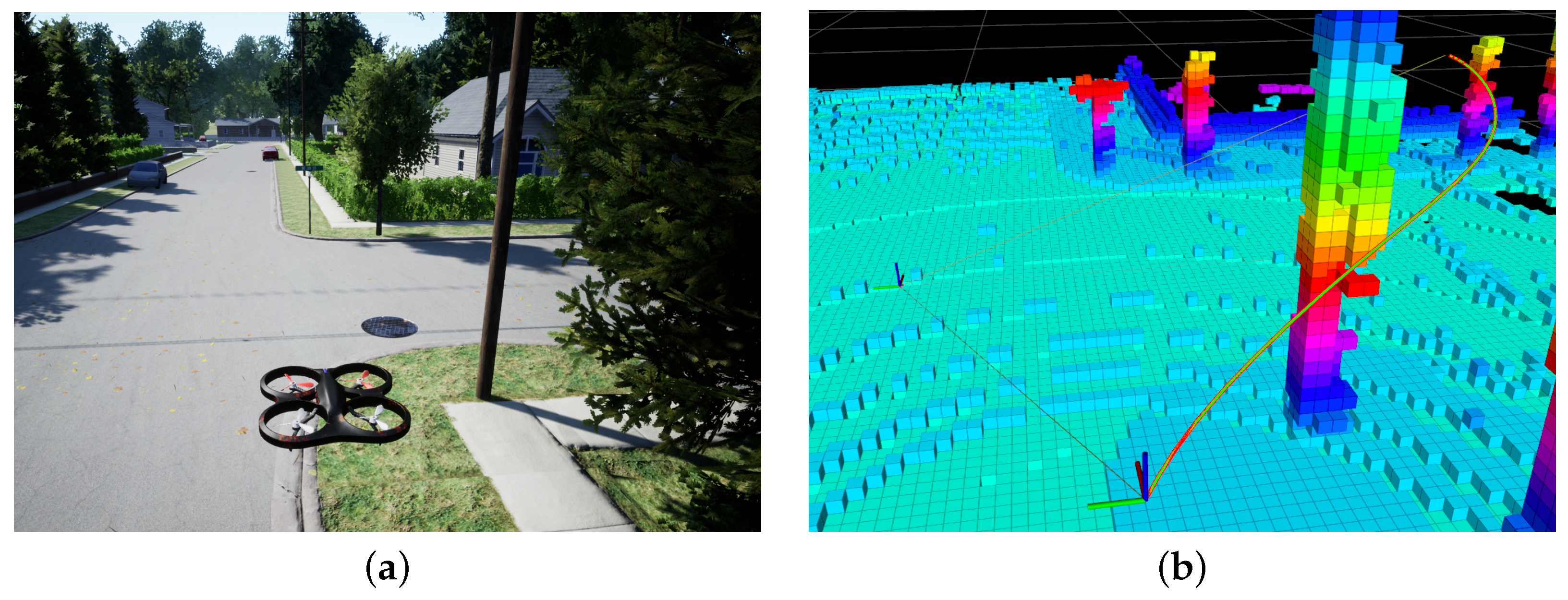
3.1. Simulation Environment

The proposed approach was first implemented in a simulation on a quadcopter drone using the AirSim simulator [45]. AirSim is an open-source package which provides photo-realistic rendered environments and a physics engine to enable performing lifelike simulations of drone vehicles. Moreover, we used the PX4 autopilot [46] running onboard the drone for software-in-the-loop operation to make the simulated drone’s characteristics more closely resemble the hardware unit.

In our work, an incremental volumetric mapping technique named Voxblox [47] was used. Voxblox represents the environment volumetrically using a signed distance field and classification into unknown, free, or occupied spaces. The drone then uses this generated map to continuously build dynamic obstacle constraints that are used by the NMPH optimization problem to generate collision-free trajectories [34].

A desktop computer equipped with an Intel Core i7-10750H CPU and an Nvidia GeForce RTX 2080 Super GPU was used to run the optimization calculations and simulation environment in conjunction with ROS. The prediction horizon of the optimization problem was set to 8.0 s and discretized into 40 samples, which was found to be sufficient for motion planning purposes. The cost function weights were empirically tuned to provide good trajectory planning performance.

The drone’s pose and environmental sensor readings were obtained from the AirSim simulator and communicated to our NMPH-based global motion planning system. The resulting output was used as a reference trajectory for the drone vehicle’s flight controller. This design enables the drone to explore an unmapped environment, as will be discussed in Section 3.1.2.

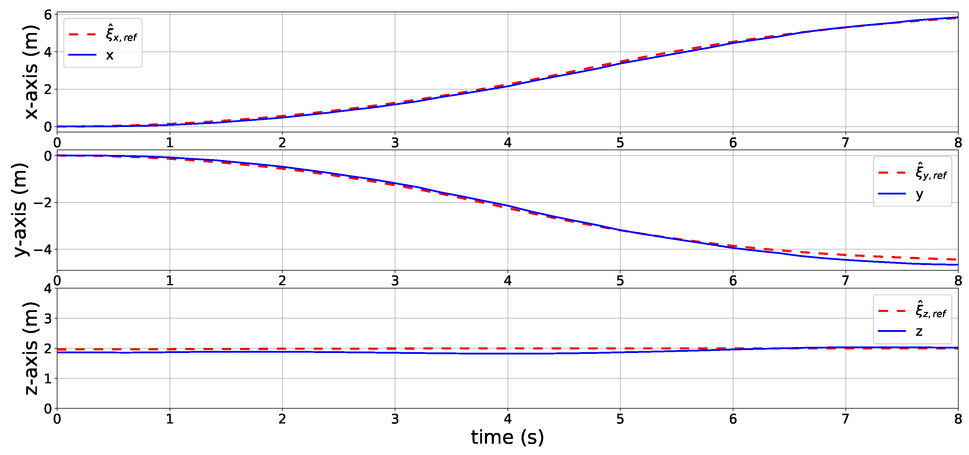
3.1.1. Trajectory Planning

In this simulation, an optimal reference trajectory was planned and tracked within the AirSim simulator as shown in Figure 3a. The quadcopter vehicle started at $p^n={[-9,-3.5,2]}^T\mathrm{m}$, $\psi =0^{\circ }$ and the NMPH-BSC algorithm was used to generate an optimal trajectory to the desired setpoint $p_d^n={[-5,-8,5]}^T\mathrm{m}$, ${\psi }_d={90}^{\circ }$ while avoiding an obstacle as shown in Figure 3b. The optimization problem within NMPH-BSC provided an estimate of the reference output trajectory ${\widehat{\xi }}_{{}_{ref}}$ and a prediction of the system state trajectory $\tilde{x}$, which included the predicted output trajectory $\tilde{\xi }$ as a subset.

Figure 4 shows that the estimated reference trajectories of the vehicle’s position and velocities ${\widehat{\xi }}_{{}_{ref}}=[{\widehat{\xi }}_{{}_{x,ref}},{\widehat{\xi }}_{{}_{y,ref}},{\widehat{\xi }}_{{}_{z,ref}},{\widehat{\xi }}_{{}_{\psi ,ref}},{\widehat{\xi }}_{{}_{\dot{x},ref}},{\widehat{\xi }}_{{}_{\dot{y},ref}},{\widehat{\xi }}_{{}_{\dot{z},ref}},{\widehat{\xi }}_{{}_{\dot{\psi },ref}}]$ perfectly match their corresponding predicted reference trajectories $\tilde{\xi }=[{\tilde{x}}_{{}_{x,ref}},{\tilde{x}}_{{}_{y,ref}},{\tilde{x}}_{{}_{z,ref}},{\tilde{x}}_{{}_{\psi ,ref}},{\tilde{x}}_{{}_{\dot{x},ref}},{\tilde{x}}_{{}_{\dot{y},ref}},{\tilde{x}}_{{}_{\dot{z},ref}},{\tilde{x}}_{{}_{\dot{\psi },ref}}]$. This confirms that using the stage cost function in (3a) minimizes the deviation between the estimated and predicted reference trajectories, and thus ensures their convergence towards each other. This validates the statement made in Section 2.1, that either the estimated or the predicted trajectory can be used as the reference trajectory for the closed-loop system.

In the second simulation, tracking performance is assessed by having the vehicle move from the initial position $p^n={[0,0,2]}^T\mathrm{m}$ to the desired terminal point $p_d={[6,-4,2]}^T\mathrm{m}$ using the optimized reference trajectory provided by the NMPH-BSC. The tracking performance is plotted in Figure 5, showing the vehicle satisfactorily tracks the time-varying reference trajectory generated by the NMPH-BSC algorithm. The small variation between the desired and actual outputs is because the former are obtained from numerical integration of the drone dynamics (10), while the latter are obtained from the physics engine of the simulation environment, which likely uses more complicated aerodynamic force and torque models than our design. This modeling mismatch can also be expected for real-world hardware testing, which will be covered in Section 3.2.

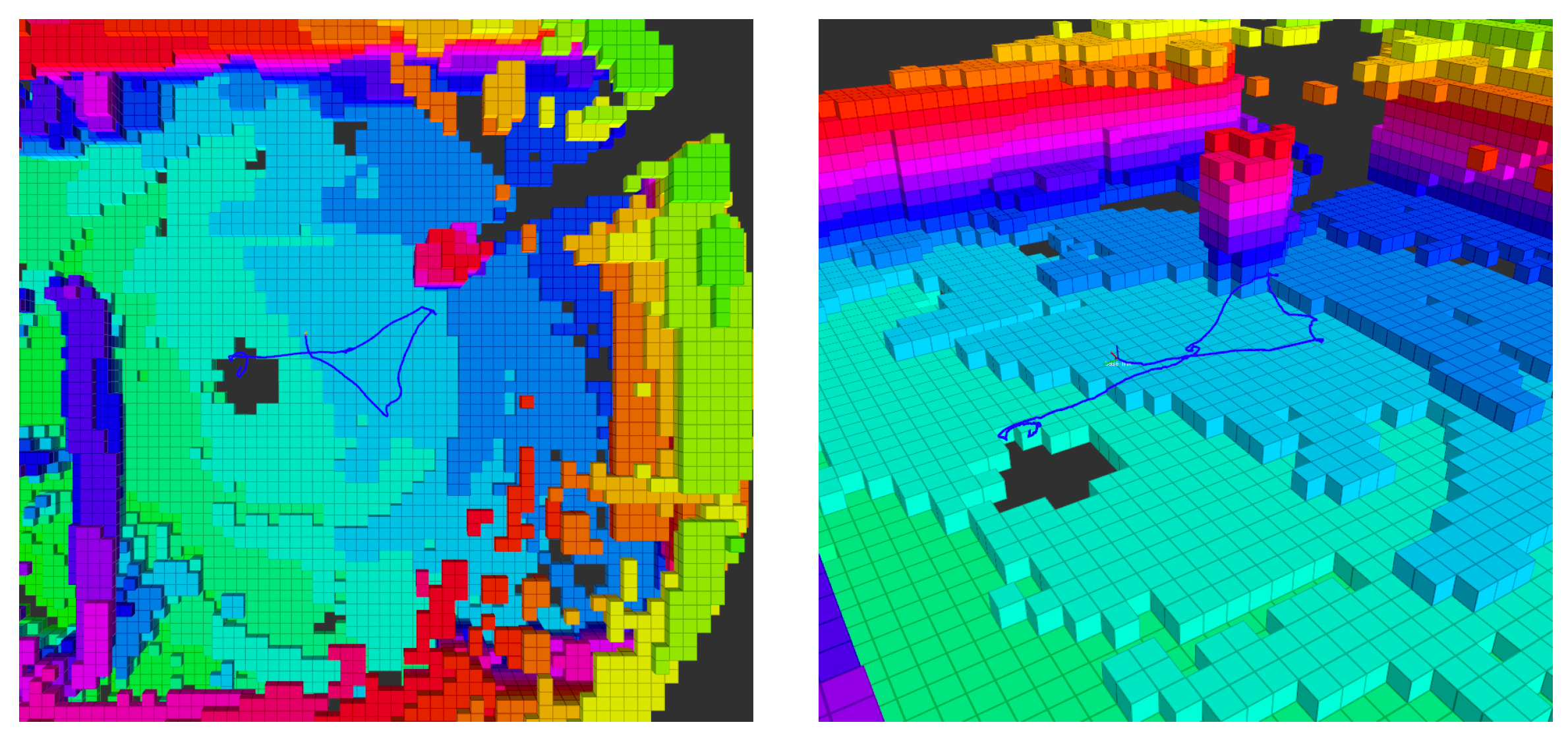
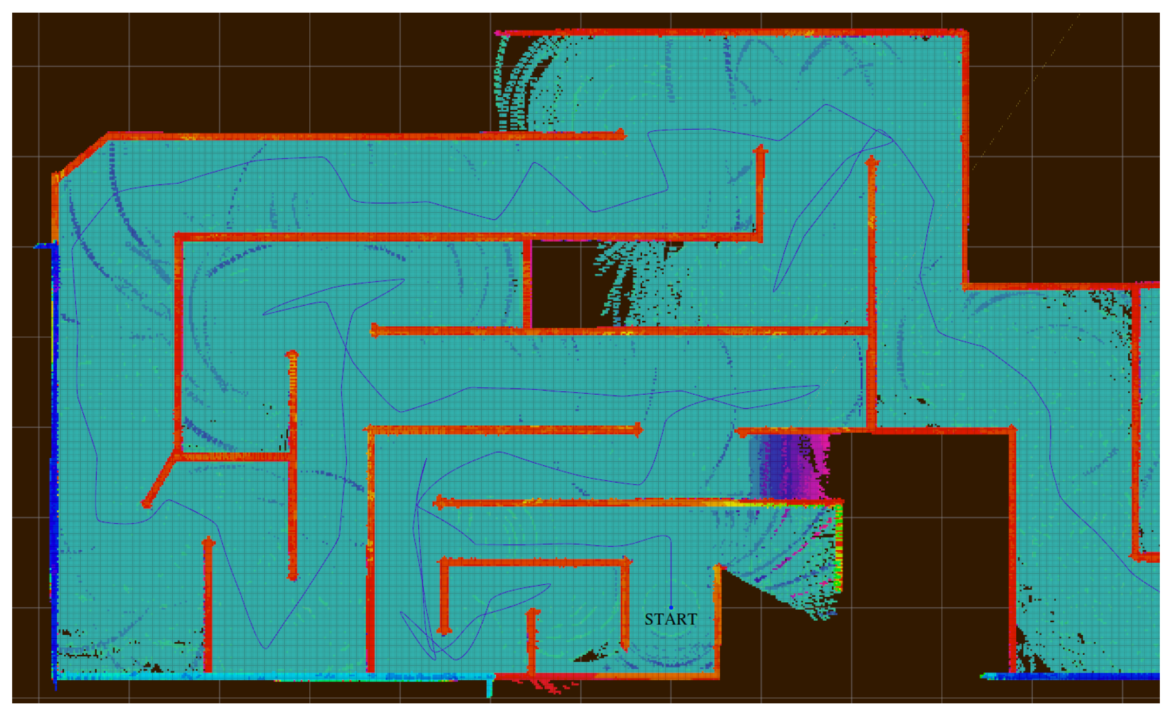
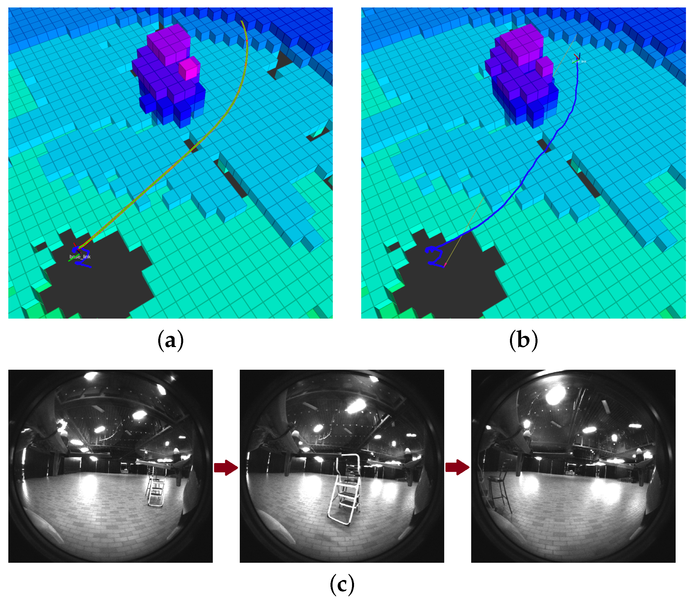
3.1.2. Exploration of Unknown Environment

In this simulation test, the drone explored an unknown environment by using a modular global motion planner, as described by the authors of [34]. This graph-based motion planner generated terminal setpoints within unexplored areas of an incrementally built-up volumetric map of the environment [47,48], and the NMPH-BSC algorithm was used to calculate optimal trajectories from the vehicle’s current pose to these terminal setpoints. To achieve a smooth integration between the graph-based planner and the NMPH-BSC trajectory planning approach, computationally efficient algorithms for obstacle mapping and avoidance plus robust path guidance algorithms were used. Further details of this methodology can be found in [34].

Figure 6 depicts a part of the exploration mission performed by the drone. The vehicle explored an unknown environment using the global motion planner in conjunction with the NMPH-BSC for local trajectory planning, which led to smoother flight trajectories than the stop-and-go patterns obtained from the motion planner alone. The data were collected over an exploration time of $1002\mathrm{s}$.

Table 1. Comparison between graph-based and graph-based-plus-NMPH approaches to motion planning.

	Total Length of the Generated Paths	Average Path Length (between Terminal Points)	Exploration Time	Continuous Path Generation
Graph-based	$1252\mathrm{m}$	$8.03\mathrm{m}$	$1322\mathrm{s}$	No
Graph-based & NMPH-FBL	$977\mathrm{m}$ (22.0% improvement)	$6.25\mathrm{m}$ (22.2% improvement)	$1032\mathrm{s}$ (21.9% improvement)	Yes
Graph-based & NMPH-BSC	$949\mathrm{m}$ (24.2% improvement)	$6.08\mathrm{m}$ (24.3% improvement)	$1002\mathrm{s}$ (24.2% improvement)	Yes

offers a comparison between three approaches: graph-based planner only [48], graph-based planner plus NMPH-FBL [27], and graph-based planner plus NMPH-BSC (this paper). Based on this comparison, it can be seen that both NMPH algorithms have the effect of reducing the distance traveled, which reduces the mission time and consequently the energy consumption of the vehicle. Using the proposed NMPH-BSC leads to an improved performance over the NMPH-FBL. This is in addition to NMPH-BSC’s advantages of avoiding numerical differentiation and its ability to extend to more complicated plant models as compared to NMPH-FBL.

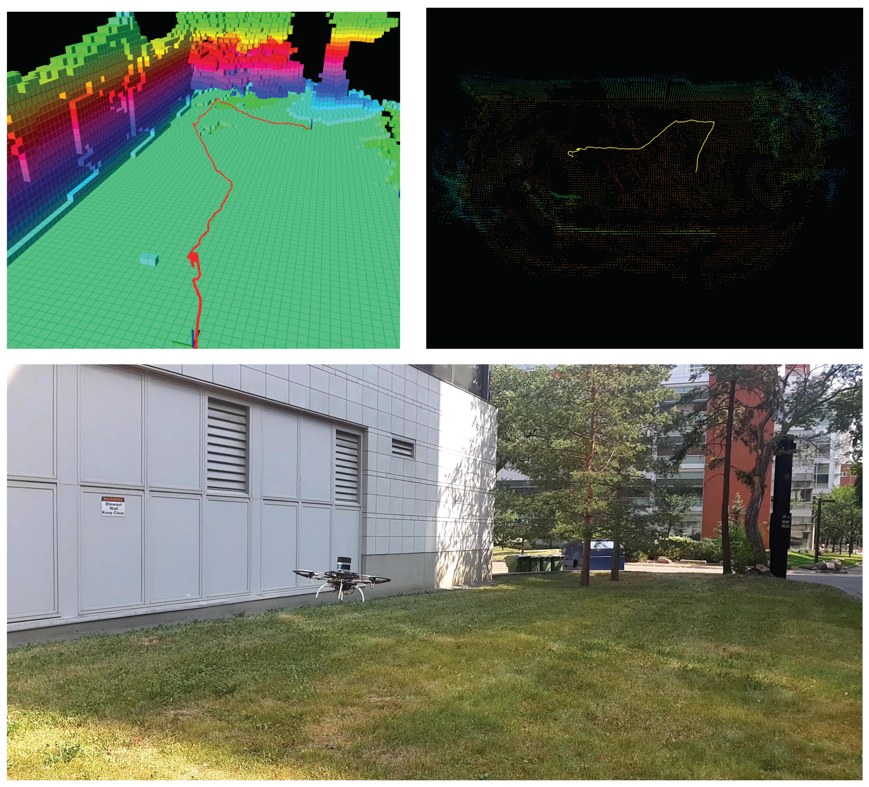
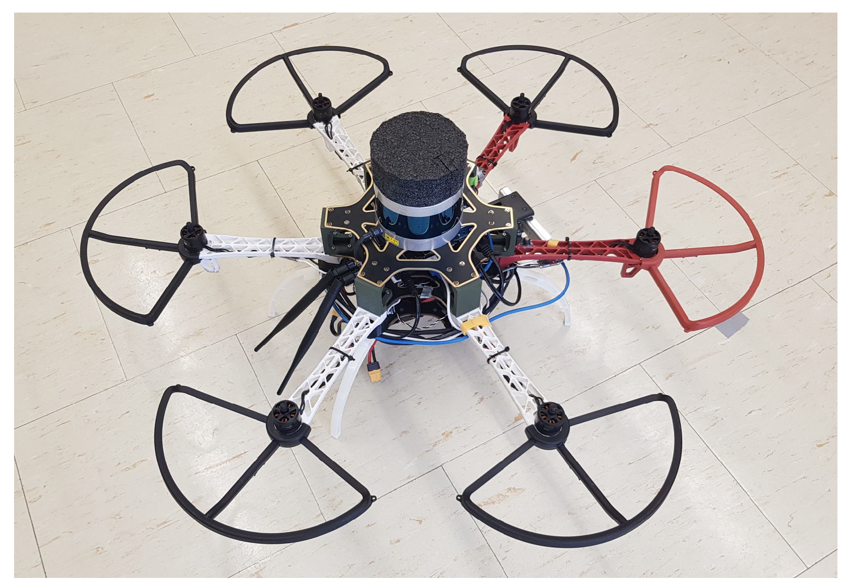
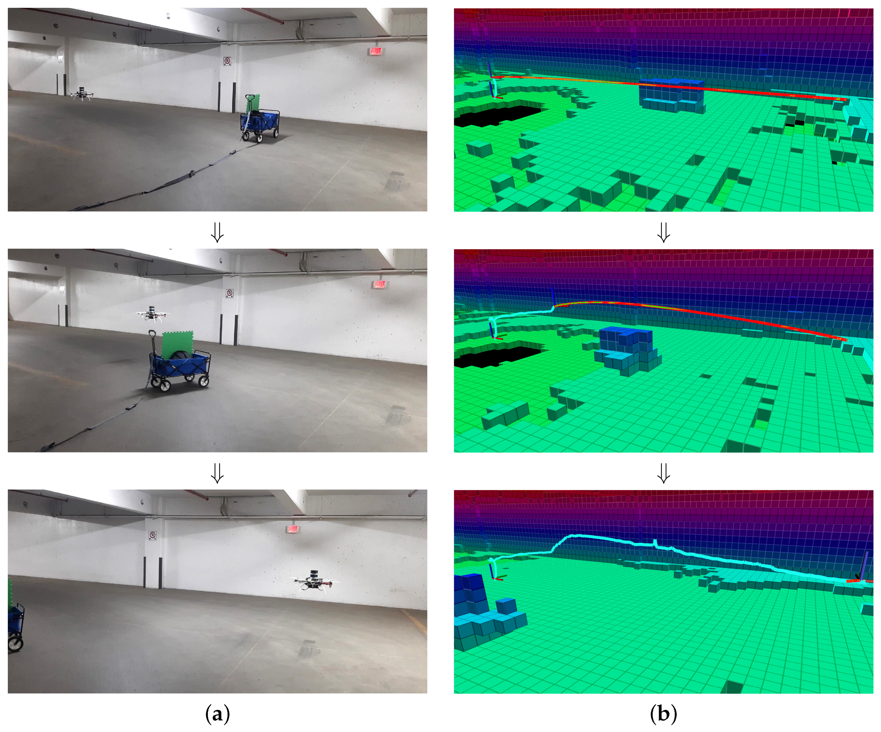
3.2. Hardware Flight Experiments

For hardware experiments, a custom DJI FlameWheel F550 hexacopter was built and instrumented to explore unknown environments using our proposed NMPH-BSC approach in conjunction with a global motion planner. The drone was equipped with a Pixhawk 2.1 flight controller running the PX4 autopilot system [46], plus an Nvidia Jetson Xavier NX system-on-module running ROS Melodic Morenia [41] under Ubuntu 18.04. A Velodyne Puck LITE LiDAR sensor and an Intel RealSense T265 stereo camera were mounted on the drone to provide ${360}^{\circ }$ point cloud and estimated pose data, respectively. The drone system used for testing is depicted in Figure 7.

Trajectory generation and tracking were evaluated by running the NMPH-BSC algorithm onboard the vehicle. Figure 8a shows the planned trajectory between two setpoints avoiding a sensed obstacle generated by the NMPH-BSC algorithm, while Figure 8b depicts the flight trajectory achieved by the drone using its flight controller to track the planned trajectory. The NMPH-BSC solver provides continuous updates of the estimated and predicted reference trajectories as the vehicle moves towards its endpoint. In this way, the system can handle uncertainties and disturbances such as dynamic environments and moving obstacles. The regeneration rate was set to 5 Hz, although this can be set as high as 100 Hz with the presented hardware.

Trajectory planning using NMPH-BSC in the presence of dynamic obstacles was evaluated experimentally as shown in Figure 9. In this Figure, it can be seen that the drone was able to regenerate trajectories to avoid a moving obstacle while flying through a constrained indoor environment. It is worth pointing out that the continuous trajectory regeneration process of NMPH-BSC provided smooth transitions between the generated trajectories, leading to smooth flight around the moving obstacle.

In a second flight test experiment, the navigation capabilities of the system were tested within a confined indoor environment as illustrated in Figure 10. During this test, the motion planner generated five terminal setpoints and the NMPH-BSC algorithm provided continuously regenerating local reference trajectories between the successive setpoints to ensure smooth flight.

A final hardware flight test was performed outdoors in order to assess the trajectory planning performance in the presence of wind, in this case approximately 15 km/h. As before, the graph-based motion planner provided multiple terminal setpoints, while our NMPH-BSC planned smooth trajectories between them in real-time. The resulting flight trajectory can be seen in Figure 11. Despite the presence of a wind disturbance, the drone was able to smoothly navigate between generated setpoints as in the earlier tests.

4. Conclusions and Future Work

This paper proposed an optimization-based trajectory planning approach for drones operating in unknown environments. The proposed method embeds the Backstepping Control technique within our recently-proposed Nonlinear Model Predictive Horizon framework [27] for generating reference trajectories for nonlinear dynamical systems. This integration reduces the non-convexity of the optimization problem and thus enables real-time computation of optimal trajectories which respect the nonlinear dynamics of the vehicle while avoiding static and dynamic obstacles.

The resulting NMPH-BSC design was tested in simulation and hardware flight experiments on quadcopter and hexacopter drone vehicles, respectively. The results showed an improvement in performance over a system previously proposed by the authors based on Feedback Linearization [34]. The new design was shown to offer additional implementation advantages over our earlier work including the ability to readily extend to more complicated plant models and avoid numerical differentiation.

Future work will include implementing an adaptation scheme allowing the online updating of the optimization problem weights within the NMPH, and testing the developed system in large-scale, unknown and GPS-denied environments such as subterranean mines.

References

1. Bergman, K.; Ljungqvist, O.; Glad, T.; Axehill, D. An optimization-based receding horizon trajectory planning algorithm. IFAC-PapersOnLine 2020, 53, 15550–15557. [Google Scholar] [CrossRef]
2. Manoharan, A.; Sharma, R.; Sujit, P.B. Multi-AAV Cooperative Path Planning using Nonlinear Model Predictive Control with Localization Constraints. arXiv 2022, arXiv:2201.09285. [Google Scholar]
3. Wu, D.M.; Li, Y.; Du, C.Q.; Ding, H.T.; Li, Y.; Yang, X.B.; Lu, X.Y. Fast velocity trajectory planning and control algorithm of intelligent 4WD electric vehicle for energy saving using time-based MPC. IET Intell. Transp. Syst. 2019, 13, 153–159. [Google Scholar] [CrossRef]
4. Gasparetto, A.; Boscariol, P.; Lanzutti, A.; Vidoni, R. Path planning and trajectory planning algorithms: A general overview. In Motion and Operation Planning of Robotic Systems; Carbone, G., Gomez-Bravo, F., Eds.; Springer: Cham, Switzerland, 2015; Volume 29, pp. 293–308. [Google Scholar]
5. Dijkstra, E.W. A note on two problems in connexion with graphs. Numer. Math. 1959, 1, 269–271. [Google Scholar] [CrossRef]
6. Hart, P.E.; Nilsson, N.J.; Raphael, B. A formal basis for the heuristic determination of minimum cost paths. IEEE Trans. Syst. Sci. Cybern. 1968, 4, 100–107. [Google Scholar] [CrossRef]
7. Koenig, S.; Likhachev, M. Fast replanning for navigation in unknown terrain. IEEE Trans. Robot. 2005, 21, 354–363. [Google Scholar] [CrossRef]
8. Al-Mutib, K.; AlSulaiman, M.; Emaduddin, M.; Ramdane, H.; Mattar, E. D* lite based real-time multi-agent path planning in dynamic environments. In Proceedings of the 2011 Third International Conference on Computational Intelligence, Modelling & Simulation, Langkawi, Malaysia, 20–22 September 2011; pp. 170–174. [Google Scholar]
9. Likhachev, M.; Gordon, G.J.; Thrun, S. ARA*: Anytime A* with provable bounds on sub-optimality. In Advances in Neural Information Processing Systems; Thrun, S., Saul, L.K., Schölkopf, B., Eds.; MIT Press: Cambridge, MA, USA, 2004; Volume 16, pp. 767–774. [Google Scholar]
10. Dolgov, D.; Thrun, S.; Montemerlo, M.; Diebel, J. Path planning for autonomous vehicles in unknown semi-structured environments. Int. J. Robot. Res. 2010, 29, 485–501. [Google Scholar] [CrossRef]
11. Siméon, T.; Laumond, J.P.; Nissoux, C. Visibility-based probabilistic roadmaps for motion planning. Adv. Robot. 2000, 14, 477–493. [Google Scholar] [CrossRef]
12. LaValle, S.M.; Kuffner, J.J. Rapidly-Exploring Random Trees: Progress and Prospects. In Algorithmic and Computational Robotics: New Directions; Donald, B.R., Lynch, K.M., Rus, D., Eds.; CRC Press: Boca Raton, FL, USA, 2001; pp. 293–308. [Google Scholar]
13. Karaman, S.; Frazzoli, E. Sampling-based algorithms for optimal motion planning. Int. J. Robot. Res. 2011, 30, 846–894. [Google Scholar] [CrossRef]
14. Khatib, O. Real-Time Obstacle Avoidance for Manipulators and Mobile Robots. Int. J. Robot. Res. 1986, 5, 90–98. [Google Scholar] [CrossRef]
15. Iswanto, I.; Ma’arif, A.; Wahyunggoro, O.; Cahyadi, A.I. Artificial Potential Field Algorithm Implementation for Quadrotor Path Planning. Int. J. Adv. Comput. Sci. Appl. 2019, 10, 575–585. [Google Scholar] [CrossRef] [Green Version]
16. Martin, P.; del Pobil, A.P. Application Of Artificial Neural Networks To The Robot Path Planning Problem. In Applications of Artificial Intelligence in Engineering IX; Adey, R., Rzevski, G., Russell, D., Eds.; WIT Press: Southampton, UK, 1994; pp. 73–80. [Google Scholar]
17. Zhao, M.; Ansari, N.; Hou, E.S.H. Mobile manipulator path planning by a genetic algorithm. J. Field Robot. 1994, 11, 143–153. [Google Scholar] [CrossRef]
18. Wang, H.J.; Xiong, W. Research on global path planning based on ant colony optimization for AUV. J. Mar. Sci. Appl. 2009, 8, 58–64. [Google Scholar] [CrossRef]
19. Qiaorong, Z.; Guochang, G. Path planning based on improved binary particle swarm optimization algorithm. In Proceedings of the 2008 IEEE Conference on Robotics, Automation and Mechatronics, Chengdu, China, 21–24 September 2008; pp. 462–466. [Google Scholar]
20. Martinez-Alfaro, H.; Flugrad, D.R. Collision-free path planning for mobile robots and/or AGVs using simulated annealing. In Proceedings of the IEEE International Conference on Systems, Man and Cybernetics, San Antonio, TX, USA, 2–5 October 1994; Volume 1, pp. 270–275. [Google Scholar]
21. Zhang, H.Y.; Lin, W.M.; Chen, A.X. Path planning for the mobile robot: A review. Symmetry 2018, 10, 450. [Google Scholar] [CrossRef]
22. Sands, T. Flattening the Curve of Flexible Space Robotics. Appl. Sci. 2022, 12, 2992. [Google Scholar] [CrossRef]
23. LaValle, S.M. Planning Algorithms; Cambridge University Press: New York, NY, USA, 2006. [Google Scholar]
24. Zucker, M.; Ratliff, N.; Dragan, A.D.; Pivtoraiko, M.; Klingensmith, M.; Dellin, C.M.; Bagnell, J.A.; Srinivasa, S.S. CHOMP: Covariant Hamiltonian optimization for motion planning. Int. J. Robot. Res. 2013, 32, 1164–1193. [Google Scholar] [CrossRef]
25. Kalakrishnan, M.; Chitta, S.; Theodorou, E.; Pastor, P.; Schaal, S. STOMP: Stochastic trajectory optimization for motion planning. In Proceedings of the 2011 IEEE international conference on robotics and automation, Shanghai, China, 9–13 May 2011; pp. 4569–4574. [Google Scholar]
26. Sandberg, A.; Sands, T. Autonomous Trajectory Generation Algorithms for Spacecraft Slew Maneuvers. Aerospace 2022, 9, 135. [Google Scholar] [CrossRef]
27. Al Younes, Y.; Barczyk, M. Nonlinear Model Predictive Horizon for Optimal Trajectory Generation. Robotics 2021, 10, 90. [Google Scholar] [CrossRef]
28. Krstic, M.; Kokotovic, P.V.; Kanellakopoulos, I. Nonlinear and Adaptive Control Design; John Wiley & Sons, Inc.: New York, NY, USA, 1995. [Google Scholar]
29. Vaidyanathan, S.; Azar, A.T. Backstepping Control of Nonlinear Dynamical Systems; Academic Press: San Diego, CA, USA, 2020. [Google Scholar]
30. Zhou, J.; Wen, C. Adaptive Backstepping Control of Uncertain Systems: Nonsmooth Nonlinearities, Interactions or Time-Variations; Springer: Heidelberg, Germany, 2008. [Google Scholar]
31. Fadhel, F.S.; Noaman, S.F. The Generalized Backstepping Control Method for Stabilizing and Solving Systems of Multiple Delay Differential Equations. Al-Nahrain J. Sci. 2018, 150–156. [Google Scholar] [CrossRef]
32. Ye, Z.; Mohamadian, H. Nonlinear backstepping control of multibody aerodynamic systems with equational modeling. In Proceedings of the 2009 IEEE International Conference on Control and Automation, Christchurch, New Zealand, 9–11 December 2009; pp. 1775–1779. [Google Scholar]
33. Marino, R.; Tomei, P. Nonlinear Control Design: Geometric, Adaptive, and Robust; Prentice Hall: Hoboken, NJ, USA, 1995. [Google Scholar]
34. Al Younes, Y.; Barczyk, M. Optimal Motion Planning in GPS-Denied Environments Using Nonlinear Model Predictive Horizon. Sensors 2021, 21, 5547. [Google Scholar] [CrossRef]
35. Murray, R.M.; Li, Z.; Sastry, S.S. A Mathematical Introduction to Robotic Manipulation; CRC Press: Boca Raton, FL, USA, 1994. [Google Scholar]
36. Madani, T.; Benallegue, A. Control of a quadrotor mini-helicopter via full state backstepping technique. In Proceedings of the 45th IEEE Conference on Decision and Control, San Diego, CA, USA, 13–15 December 2006; pp. 1515–1520. [Google Scholar]
37. Al Younes, Y.; Drak, A.; Noura, H.; Rabhi, A.; Hajjaji, A.E. Quadrotor position Control using cascaded adaptive integral backstepping controllers. In Applied Mechanics and Materials; Trans Tech Publications Ltd.: Durnten-Zurich, Switzerland, 2014; Volume 565, pp. 98–106. [Google Scholar]
38. Bouabdallah, S.; Siegwart, R. Full control of a quadrotor. In Proceedings of the 2007 IEEE/RSJ international conference on intelligent robots and systems, San Diego, CA, USA, 29 October–2 November 2007; pp. 153–158. [Google Scholar]
39. Basri, M.A.M.; Husain, A.R.; Danapalasingam, K.A. Enhanced backstepping controller design with application to autonomous quadrotor unmanned aerial vehicle. J. Intell. Robot. Syst. 2015, 79, 295–321. [Google Scholar] [CrossRef]
40. Chen, F.; Jiang, R.; Zhang, K.; Jiang, B.; Tao, G. Robust backstepping sliding-mode control and observer-based fault estimation for a quadrotor UAV. IEEE Trans. Ind. Electron. 2016, 63, 5044–5056. [Google Scholar] [CrossRef]
41. Quigley, M.; Gerkey, B.; Conley, K.; Faust, J.; Foote, T.; Leibs, J.; Berger, E.; Wheeler, R.; Ng, A.Y. ROS: An open-source Robot Operating System. ICRAWorkshop on Open Source Software in Robotics, Kobe, Japan, 12–17 May 2009. [Google Scholar]
42. Houska, B.; Ferreau, H.; Diehl, M. ACADO Toolkit—An Open Source Framework for Automatic Control and Dynamic Optimization. Optim. Control Appl. Methods 2011, 32, 298–312. [Google Scholar] [CrossRef]
43. Boggs, P.T.; Tolle, J.W. Sequential quadratic programming. Acta Numer. 1995, 4, 1–51. [Google Scholar] [CrossRef]
44. Ferreau, H.; Kirches, C.; Potschka, A.; Bock, H.; Diehl, M. qpOASES: A parametric active-set algorithm for quadratic programming. Math. Program. Comput. 2014, 6, 327–363. [Google Scholar] [CrossRef]
45. Shah, S.; Dey, D.; Lovett, C.; Kapoor, A. AirSim: High-Fidelity Visual and Physical Simulation for Autonomous Vehicles. In Field and Service Robotics; Hutter, M., Siegwart, R., Eds.; Springer: Cham, Switzerland, 2018; pp. 621–635. [Google Scholar]
46. Meier, L.; Honegger, D.; Pollefeys, M. PX4: A node-based multithreaded open source robotics framework for deeply embedded platforms. In Proceedings of the 2015 IEEE International Conference on Robotics and Automation (ICRA), Seattle, WA, USA, 26–30 May 2015; pp. 6235–6240. [Google Scholar]
47. Oleynikova, H.; Taylor, Z.; Fehr, M.; Siegwart, R.; Nieto, J. Voxblox: Incremental 3d euclidean signed distance fields for on-board mav planning. In Proceedings of the 2017 IEEE/RSJ International Conference on Intelligent Robots and Systems (IROS), Vancouver, BC, Canada, 24–28 September 2017; pp. 1366–1373. [Google Scholar]
48. Dang, T.; Mascarich, F.; Khattak, S.; Papachristos, C.; Alexis, K. Graph-based path planning for autonomous robotic exploration in subterranean environments. In Proceedings of the 2019 IEEE/RSJ International Conference on Intelligent Robots and Systems (IROS), Macau, China, 4–8 November 2019; pp. 3105–3112. [Google Scholar]
Figure 1. NMPH Architecture. The NMPH optimization process (gray box) considers models of the nonlinear plant dynamics and nonlinear control law, as well as constraints representing performance limits and environmental obstacles. The actual closed-loop system (blue box) tracks the optimized reference trajectory calculated by NMPH.
Robotics 11 00087 g001
Figure 2. Reference frames used for our quadrotor vehicle.
Robotics 11 00087 g002
Figure 3. Trajectory Planning using the NMPH-BSC approach. (a) AirSim simulation environment. (b) Trajectory generation while avoiding static obstacle.
Robotics 11 00087 g003
Figure 4. NMPH reference trajectory generation. The estimated and predicted reference position trajectories are depicted in (a), and the estimated reference velocity trajectories are shown in (b).
Robotics 11 00087 g004
Figure 5. Vehicle’s trajectory tracking performance between the start point (0, 0, 2) m and the terminal setpoint (5.8, −4.5, 2) m.
Robotics 11 00087 g005
Figure 6. Exploration of unknown environment using global motion planner using NMPH-BSC for local trajectory planning.
Robotics 11 00087 g006
Figure 7. DJI FlameWheel F550 hexacopter vehicle equipped with onboard sensors and computing systems.
Robotics 11 00087 g007
Figure 8. Trajectory planning with obstacle avoidance flight test using the NMPH-BSC algorithm. (a) Trajectory generation. (b) Trajectory tracking. (c) The mapped obstacle as seen from the left fisheye lens of the onboard camera.
Robotics 11 00087 g008
Figure 9. Hardware flight test for trajectory planning involving a dynamic obstacle using the NMPH-BSC algorithm. (a) Hardware drone avoiding the moving obstacle. (b) RViz visualization of the trajectory regeneration and flight path.
Robotics 11 00087 g009
Figure 10. The hardware hexacopter vehicle navigating a confined indoor environment using a graph-based planner to generate terminal setpoints and NMPH-BSC to generate local trajectories between setpoints.
Robotics 11 00087 g010
Figure 11. Flight test employing the NMPH-BSC algorithm in an outdoor environment with a 15 km/h wind speed.
Robotics 11 00087 g011