Robust Trajectory-Tracking for a Bi-Copter Drone Using INDI: A Gain Tuning Multi-Objective Approach

Abstract

This paper presents an optimized robust trajectory control system for an autonomous tiltrotor bi-copter based on an incremental nonlinear dynamic inversion (INDI) strategy combined with a set of PID/PD controllers. The methodology includes a lower level, fast attitude control action using an incremental nonlinear dynamic inversion (INDI) strategy, which is driven by a higher level, slow trajectory control action that uses nonlinear dynamic inversion (NDI). The nonlinear dynamic model of the drone is derived, and the basis of the motion and the design of the attitude and position stabilizing controllers are discussed. To develop and test the suggested controller, a circle-shaped flight profile is simulated. The linear control providing inputs to the NDI and INDI controllers is tuned via a novel multi-objective optimization auto-tuning method using the non-dominated sorting genetic algorithm II (NSGA-II). The tracking and disturbance rejection optimization is achieved via the use of the integral of time multiplied by the absolute error (ITAE) and the integral of the square of the error (ISE) objective functions, which are optimized concurrently. The simulation results reveal that the proposed control design outperforms the traditional dynamic inversion controller design and demonstrate that the developed INDI + PID/PD controller possesses exceptional accuracy and performance, enabling the tiltrotor bi-copter to track the given trajectory. Furthermore, the paper shows that the proposed controller produces 40% lower overshoot and settling time as measured with respect to previous backstepping controllers reported in the literature. The robustness of the controller is validated through diverse tests where the aircraft is subjected to external (wind gust) disturbances.

1. Introduction

Multi-rotor drones and their novel structures and designs have been an attractive topic for researchers and industries in recent years. Typical multi-rotor drones have four, six, and eight rotors and can be controlled to perform different maneuvers by changing their propellers’ speed. They have been used in a wide variety of applications such as search and rescue [1,2], agriculture [3,4], data collection and monitoring [5,6], health assistance missions (for COVID-19) [7], and many other tasks. However, due to their high power requirements, their nonlinearities, and coupled flight effects, multi-rotor drones usually have short mission times and are difficult to control, especially under the presence of internal (e.g., failures) and external (e.g., wind) disturbances. Therefore, a new configuration of multi-rotor drones with two motors/propellers that can reduce the unit time power demand was introduced in [8]. By reducing the number of propellers, bi-copter airframes not only provide a less power-hungry eVTOL (Electric Vertical Take-off and Landing) aircraft but the aerodynamic interaction of the propellers with the fuselage and the ground (aerodynamic wall and ground effects) decreases, thus reducing the typical adverse effects during flight. Similar drones have enhanced flying acrobatic capabilities not seen in typical eVTOL systems (e.g., pitched hover); they have also been developed to fly inside confined spaces using diverse control schemes [9,10,11]. Although such aircraft are complex, they provide the characteristics for developing and testing new control strategies that can be extended to control other VTOL vehicles having advanced flight capabilities, such as the highly maneuverable drones for confined spaces developed at the University of Calgary [12]. Although the aircraft introduced in [8] is relatively simple when compared to other tiltrotor aircraft (e.g., [12] and V-22 Osprey), it is a nonlinear system [13], and has the ability, at least in theory, to maneuver through small spaces providing a suitable testbed platform to develop and test concept (enhanced) controllers for sophisticated eVTOL aircraft systems.

Several works have developed traditional PID controllers for position and attitude tracking of bi-copter drones [8,14,15,16]. Although somewhat effective, such techniques have a number of drawbacks. For starters, a linearized model of the aircraft is typically used, which provides an approximation of the behavior and flight capabilities of such systems. To really exploit the capabilities of such systems, nonlinear models should be used that describe the motion-coupling and aerodynamic effects inherited by the flying mechanisms. Second, any linearized model is only viable within minor deviations from the equilibrium or trim point. Thus, performance can suffer significantly if the aircraft drifts away from its intended design/flight trim point. As a result, gain scheduling is frequently used to achieve somewhat acceptable performance across the whole flight envelope.

A variety of nonlinear flight control systems have been proposed and developed in the hopes of overcoming some of the theoretical constraints and downsides of linear controller design. Examples of nonlinear control methods to control the motion of flying robots include feedback linearization [17], backstepping [10,13,18,19], predictive [9,20,21], and sliding mode control [22,23,24]. Although these methods provide the ability to control drones in different conditions, they are highly dependent on the accuracy of the vehicle’s dynamic model. Furthermore, such controllers also have limited capability to cope with unknown internal or external disturbances affecting the aircraft flight and the uncertainties (accuracy) of the mathematical model.

Among such controllers, the feedback linearization technique has attracted the most attention as it has proven to have the most potential to control diverse Unmanned Aerial Vehicles (UAVs) [25]. The most important feature of the associated synthesis process for this type of controller is that gain scheduling is no longer required. A characteristic that other controllers share.

Nonlinear dynamic inversion (NDI) is a feedback linearization candidate methodology that aims to remove gain scheduling by inverting and canceling the inherent dynamics and replacing them with a set of user-selected desirable dynamics [26]. Because of these factors, NDI is a promising control design method extending the capabilities of other control techniques, especially for aircraft having large flight maneuvering envelopes. However, the main challenge in using feedback linearization for air vehicle control is that it necessitates extensive knowledge of the nonlinear dynamic model of the system and, therefore, cannot deal with the uncertainties [27]. Because these are approaches based on system knowledge, they are referred to as model-based solutions. However, the model accuracy requirement can be costly and time-consuming. In the case of aircraft control, where there are a number of uncertainties, such as aerodynamic coefficients (coefficients that change based on the flight maneuver being performed), extensive wind tunnel tests as well as flight and CFD studies are required to be able to properly generate the needed aircraft’s mathematical model.

Because of the general advancement of micro-electromechanical systems (MEMS), smaller, more accurate, and more accessible sensors are now available. This enables sensor-based control approaches in which model knowledge can be replaced by variable measurements to be developed. Incremental nonlinear dynamics inversion (INDI) is one such sensor-based control approach [28,29,30,31] in which the incremental control input replaces the total control input used in NDI. For this, the incremental control input is calculated based on the performance of the system in the previous time step via sensor measurements. Therefore, INDI is less dependent on the dynamic model of the system and model uncertainties. However, this technique is required to be executed at a high-frequency using accurate sensor data and/or accurate variable estimation.

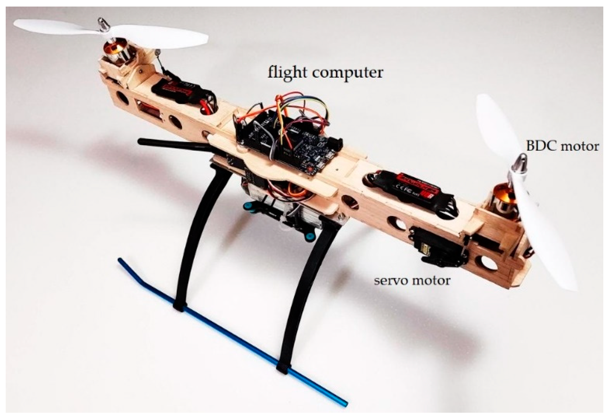
In this paper, a nonlinear mathematical model of the bi-copter presented in [13] and shown in Figure 1 is developed.

The control architecture includes the development of a novel multi-loop trajectory controller designed based on INDI and PID controller formulations. First, an inner-loop controller is designed for high-performance attitude tracking, followed by the development of an outer loop that tracks position variables via an NDI controller. The outer loop generates attitude commands that appropriately orient the tilting rotor forces to generate the required translational accelerations. This two-loop control approach generally requires timescale separation where the outer-loop bandwidth must be significantly lower than the inner-loop bandwidth. Following the typical system linearization performed in INDI (or NDI), it is now possible to use the linear control to stabilize each state of the UAV (position and orientation) separately.

PID controllers have been developed and used in diverse fields such as industrial control, energy, as well as in the control of unmanned aircraft. However, optimizing the three parameters required in any PID controller is a difficult task, especially when several performance indices are to be met at the same time. There exist several common methodologies, including Pole placement and Lyapunov theory, to obtain linear control parameters for a given system, including the control gains to use, but there is not an accurate method of tuning these parameters [32].

In the area of UAVs, diverse methods have been developed to obtain optimal parameters (e.g., gains) for numerous aircraft. Examples of such techniques include Min–Max parameter optimization, where researchers have used DI airplane flight controller (e.g., [32]), and fuzzy proportional/integral/derivative (fuzzy-PID) design [33].

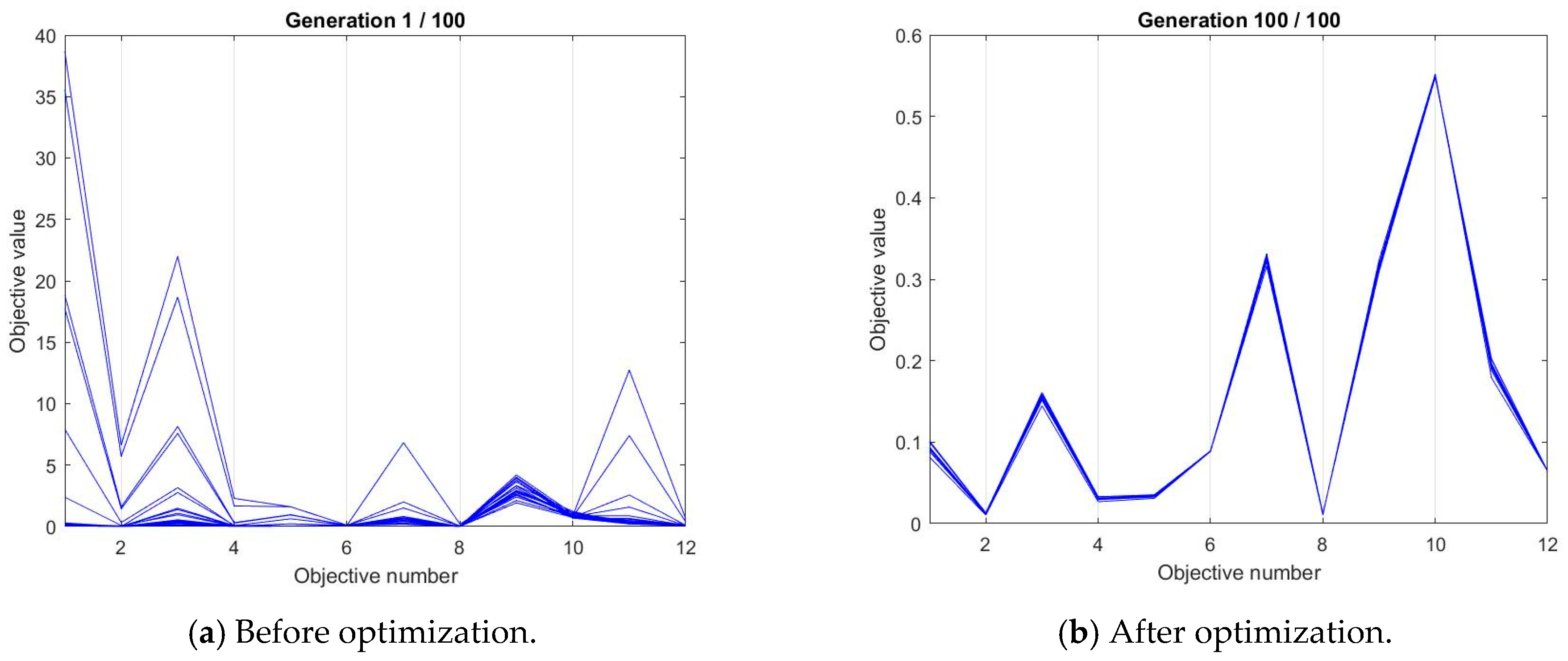
In this paper, the NSGA-II optimization algorithm is used to optimize the PID parameters of the bi-copter’s INDI controller. According to [34], NSGA-II can find a much wider range of solutions and converge closer to the true optimal solution when compared to other evolutionary algorithms (EA).

In this paper, a bi-copter drone similar to the one presented in [21] is used to develop a novel INDI controller for autonomous operation. Due to the complexities associated with the control of such a drone concept (e.g., coupled dynamics), prior work only considered the development of a backstepping (BKS) controller to operate the aircraft under benign flight conditions [21] and tracking relatively simple trajectories (defined as a set of points in 3D space) without explicit system (drone) orientation. Since BKS requires explicit system model information, such a solution was highly sensitive to model uncertainties and prone to poor disturbance rejection. This paper provides an improved control solution based on the combination of the incremental nonlinear dynamic inversion (INDI) strategy with simple PID controllers, which reduces model dependency and enhances disturbance rejection. The proposed controller is a novel architecture that can be easily applied to diverse systems beyond autonomous aircraft, especially those with complex dynamics operating in the presence of inner and/or outer disturbances, such as wind gusts and system failures. The proposed control architecture employs an offline optimization technique to tune the required PID control gains, which provides effective results even with minimal tuning efforts.

The paper is divided into four sections: Section 2 extracts the bi-copter’s nonlinear mathematical model; Section 3 describes the proposed dynamic inversion method and Section 4 describes the NSGA-II optimization algorithm. Numerical simulations are presented in Section 5, followed by the conclusions in Section 6.

2. Dynamic Model: Tiltrotor Bi-Copter

2.1. Flight Mechanism

The drone that is the subject of this paper is a six degrees-of-freedom (DOF) dual rotor drone, bi-copter, with tilting rotors (Figure 1). The aircraft has four control inputs, w₁, w₂, t₁, and t₂, which correspond to the left/right propellers’ speed and their corresponding tilt angles around the y-axis of the vehicle’s body frame (Figure 2).

The aircraft, having a mass “m”, is able to fly sideways as well as forward and backward by the control of the four control inputs. The motion sideways (in the “y”-direction, see Figure 2) is obtained by generating a differential thrust/speed of the propellers. By changing the tilt angles, $t_i$, of the propellers in equal amounts fore and aft, motion is achieved (i.e., motion in “x”-direction). Yaw motion (i.e., rotation about the vehicle’s “z”-axis) is achieved by the differential tilt angle of the propellers. The described motions are, however, coupled. For example, during sideways motion, the differential rotational speeds of the propellers will also generate roll and yaw motions. In other cases, the gyroscopic effects of the tilting propellers will also cause a coupled pitch motion of the UAV.

2.2. Dynamic Model

In order to derive a dynamic model of the system, the Newton–Euler formulation is used. For this, two frames of reference are used: An inertial reference frame,$X_I{Y}_I{Z}_I$, and a body reference frame, $X_B{Y}_B{Z}_B$, as shown in Figure 2 with the transformation matrix from the inertial reference frame to the body reference frame denoted as $R_B^I$ (Equation (1)). Furthermore, for the modeling of the aircraft, the Euler angles ($\phi , \theta , \psi$⇒ roll, pitch, yaw) used to denote and represent the motion of the aircraft with respect to the inertial frame of reference were used. Such angles denote the rotational speeds and tilt angles of the left and right motors, respectively. In what follows, the subscripts 1 and 2 are used to represent the left and right propellers of the aircraft, respectively, as well as the corresponding parameters (e.g., ω_i for the rotational speed of propeller “i”).

$$R_B=\left[\begin{array}{c} cos\theta cos\psi cos\theta sin\psi -sin\theta \\ -cos\varphi sin\psi +sin\varphi sin\theta cos\psi cos\varphi cos\psi +sin\varphi sin\theta sin\psi sin\varphi cos\theta \\ sin\varphi sin\psi +cos\varphi sin\theta cos\psi -sin\varphi cos\psi +cos\varphi sin\theta sin\psi cos\varphi cos\theta \end{array}\right]$$

(1)

The relationship between the angular velocity of the aircraft with respect to the inertial frame (p, q, r), and the first derivative of the Euler angles is:

$$\left[\dot{\begin{array}{c}\varphi \\ \dot{\begin{array}{c}\theta \\ \dot{\psi }\end{array}}\end{array}}\right]=\left[\begin{array}{c}1 tan\theta sin\varphi tan\theta cos\varphi \\ 0 cos\varphi -sin\varphi \\ 0 sin\varphi /cos\theta cos\varphi /cos\theta \end{array}\right]\left[\begin{array}{c}p\\ q\\ r\end{array}\right]$$

(2)

In order to simplify the equations of motions, the following four assumptions are employed: (i) the center of the mass of the UAV and the body reference frame coincide, (ii) the structure of the drone is symmetric to the XZ (longitudinal) plane so that $I_{XY}=0$ and $I_{ZY}=0$, (iii) the aerodynamic coefficients such as drag do not change, and (iv) the forces created by the propellers are proportional to the square of their rotation speed. Furthermore, the drag forces of propellers are considered negligible.

Based on the above-described aspects, the equation of the motion for the bi-copter is formulated as described in Equation (3):

$$\{\begin{array}{c}\ddot{x}=-\frac{sin\varphi sin\psi +cos\varphi sin\theta cos\psi }{m}{C}_T\left({\omega }_1^{2}cos{t}_1+{\omega }_2^{2}cos{t}_2\right)\\ -\frac{cos\theta cos\psi }{m}{C}_T\left({\omega }_1^{2}sin{t}_1+{\omega }_2^{2}sin{t}_2\right)\\ \ddot{y}=\frac{sin\varphi cos\psi -cos\varphi sin\theta sin\psi }{m}{C}_T\left({\omega }_1^{2}cos{t}_1+{\omega }_2^{2}cos{t}_2\right)+\\ \frac{cos\theta sin\psi }{m}{C}_T\left({\omega }_1^{2}sin{t}_1+{\omega }_2^{2}sin{t}_2\right)\\ \ddot{z}=-\frac{cos\varphi cos\theta }{m}{C}_T\left({\omega }_1^{2}cos{t}_1+{\omega }_2^{2}cos{t}_2\right)-\\ \frac{sin\theta }{m}{C}_T\left({\omega }_1^{2}sin{t}_1+{\omega }_2^{2}sin{t}_2\right)+g\\ \dot{p}=\frac{I_{XZ}}{I_{XX}}\left(\dot{r}+pq\right)+\frac{I_{YY}-I_{ZZ}}{I_{XX}}qr+\frac{l{C}_T\left({\omega }_1^{2}cos{t}_1-{\omega }_2^{2}cos{t}_2\right)}{I_{XX}}\\ \dot{q}=\frac{I_{XZ}}{I_{YY}}\left(r^2-p^2\right)+\frac{I_{ZZ}-I_{XX}}{I_{YY}}pr+\frac{h{C}_T\left({\omega }_1^{2}sin{t}_1+{\omega }_2^{2}sin{t}_2\right)}{I_{YY}}\\ \dot{r}=\frac{I_{XZ}}{I_{ZZ}}\left(\dot{p}-qr\right)+\frac{I_{XX}-I_{YY}}{I_{ZZ}}pq+\frac{l{C}_T\left({\omega }_1^{2}sin{t}_1-{\omega }_2^{2}sin{t}_2\right)}{I_{ZZ}}\end{array}$$

(3)

where C_T is the thrust coefficient of the motors, ${\omega }_1$ and ${\omega }_2$ are the rotational speeds of the left and right propellers, respectively, l and h are the horizontal and vertical distances of the rotors to the center of the mass of the UAV, respectively, and, $t_i$, represents the tilt angle of the propellers “i” (see Figure 1 and Figure 2) [8]. In order to simplify these coupled sets of equations (Equation (3)), the four control variables $U_1, U_2, U_3, U_4$ are defined as shown in Equation (4). Then Equation (3) can be rewritten as Equation (5).

$$U=\left[\begin{array}{c}{U}_1\\ U_2\\ U_3\\ U_4\end{array}\right]=\left[\begin{array}{c}{C}_T\left({\omega }_1^{2}cos{t}_1+{\omega }_2^{2}cos{t}_2\right)\\ C_T\left({\omega }_1^{2}cos{t}_1-{\omega }_2^{2}cos{t}_2\right)\\ C_T\left({\omega }_1^{2}sin{t}_1+{\omega }_2^{2}sin{t}_2\right)\\ C_T\left({\omega }_1^{2}sin{t}_1-{\omega }_2^{2}sin{t}_2\right)\end{array}\right]$$

(4)

$$\{\begin{array}{c}\ddot{x}=-\frac{U_1}{m}\left(sin\varphi sin\psi +cos\varphi sin\theta cos\psi \right)-\\ \frac{cos\theta cos\psi }{m}{U}_3\\ \ddot{y}=\frac{U_1}{m}\left(sin\varphi cos\psi -cos\varphi sin\theta sin\psi \right)+\\ \frac{cos\theta sin\psi }{m}{U}_3\\ \ddot{z}=-cos\varphi cos\theta \frac{U_1}{m}-\frac{sin\theta }{m}{U}_3+g \\ \dot{p}=\frac{I_{XZ}}{I_{XX}}\left(\dot{r}+pq\right)+\frac{I_{YY}-I_{ZZ}}{I_{XX}}qr+\frac{l{U}_2}{I_{XX}} \\ \dot{q}=\frac{I_{XZ}}{I_{YY}}\left(r^2-p^2\right)+\frac{I_{ZZ}-I_{XX}}{I_{YY}}pr+\frac{h{U}_3}{I_{YY}} \\ \dot{r}=\frac{I_{XZ}}{I_{ZZ}}\left(\dot{p}-qr\right)+\frac{I_{XX}-I_{YY}}{I_{ZZ}}pq+\frac{l{U}_4}{I_{ZZ}} \end{array}$$

(5)

The kinetic model, expressed by Equation (5), is then used to develop the corresponding controller, which is then implemented in the MATLAB/Simulink simulation environment where testing and analyzing of the flight controller is performed.

3. Controller Design

Aircraft do not always behave as linear systems. This is especially true when performing aggressive maneuvers or experiencing internal or external disturbances or when the aircraft’s design is non-traditional such as bi-copters and tiltrotor aircraft. Thus, in some flight regimes, including failure scenarios, they behave in a nonlinear fashion. To control them effectively and efficiently, one must use nonlinear controllers. Such controllers must also be robust, as the mathematical models used to derive the corresponding controller never exactly matches the real-world system.

In this paper, nonlinear dynamic inversion (NDI) and incremental NDI (INDI) are considered. The reason is that such controllers have been proven to perform much better than linear controllers (e.g., PID) in terms of disturbance rejection [28,29] (as one example) and are easier to use for controlling nonlinear systems. Moreover, such controllers offer the possibility for very robust control.

3.1. Controller Formulation

3.1.1. Nonlinear Dynamics Inversion

Considering the general equation of the motion for a Multi Input Multi Output (MIMO) system [35], the equation of the motion of the bi-copter tiltrotor UAV has the following form (Equations (6) and (7)):

$$\dot{x}=f\left(x\right)+G\left(x\right)u$$

(6)

$$y=h\left(x\right)$$

(7)

where $x\in R^n$ is the system’s state vector, $u\in R^m$ is the control input vector, $f\left(x\right)\in R^n$ and $h\left(x\right)\in R^m$ are smooth nonlinear vector fields (functions), and $G\left(x\right)\in R^{n\times m}$ is one of the system’s model matrix where each column contains values defined as $g_i\in R^n$.

By differentiating Equation (7) with respect to time, Equation (8) is obtained:

$$\dot{y}=\frac{dh\left(x\right)}{dt}=\frac{\partial h}{\partial x}\dot{x}=\frac{\partial h}{\partial x}f\left(x\right)+\frac{\partial h}{\partial x}G\left(x\right)u=L_{f}h\left(x\right)+L_{G}h\left(x\right)u$$

(8)

where $L_{f}h\left(x\right)$ and $L_{G}h\left(x\right)$ are the Lie Derivatives of $h\left(x\right)$ with respect to $f$ and $G$, respectively. Assuming $L_{G}h\left(x\right)$ is invertible, it is possible to isolate the (virtual) control action u as shown in Equation (9).

$$u={\left(L_{G}h\left(x\right)\right)}^{-1}\left(\dot{y}-L_{f}h\left(x\right)\right)$$

(9)

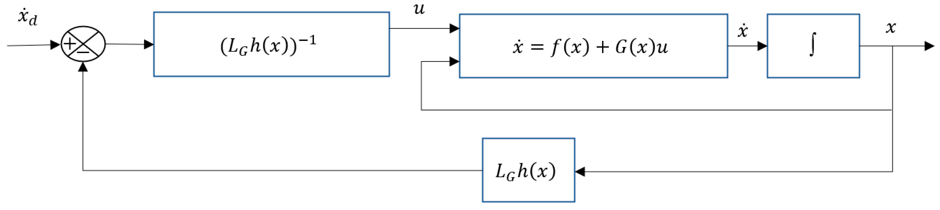
Equation (9) uses a reasonable assumption, which guarantees that the function $L_{G}h\left(x\right)$ satisfies the zero typical conditions of the $\mathit{det}(L_{G}h\left(x\right))$ while avoiding unfeasible system configurations. This is possible by defining limitations to the equations describing the aircraft’s behavior. In turn, such determinants can be easily obtained via a pseudo-inverse computation to avoid any singularity of the controller. Applying this control action to (6) results in a closed-loop linearized system of the form $\dot{x}={\dot{x}}_d$. A block diagram describing such an approach is presented in Figure 3.

Although effective, the linearization process described above has limitations derived from the relative degree of each output y and the rank of matrix $G\left(x\right)$. For the purpose of this paper, the relative degree of an output denotes the number of differentiations needed to capture a given input (also known as the control command) u explicitly in terms of $h\left(x\right)$. If there are outputs having higher relative degrees when compared to the other outputs, then it is possible to linearize them directly with either NDI or INDI. The rank of $G\left(x\right)$ can also be used to represent the number of state’s derivatives $\dot{x}$ that are directly affected by the control action u. If this rank k is not equal to the total number of states n, then (n − k) states cannot be linearized directly (i.e., zero dynamics states).

3.1.2. Incremental Nonlinear Dynamics Inversion

In contrast to NDI, INDI has no requirements for input dynamics. Thus, it is possible to use a more generic formulation for nonlinear systems, as requested by Equation (10), where $F\left(x,u\right)$ is a nonlinear function:

$$\dot{x}=F\left(x,u\right)$$

(10)

If the model described by Equation (10) is used to develop a controller running with a sampling time, ∆T, it is possible to linearize Equation (10) around the previous time step, t₀ = t − ∆T, where the system’s state was defined by (x₀, u₀), as represented by Equation (11).

$$\dot{x}={\dot{x}}_0+\frac{\partial F}{\partial x}{|}_{x_0,u_0}\left(x-x_0\right)+\frac{\partial F}{\partial u}{|}_{x_0,u_0}\left(u-u_0\right)$$

(11)

where ${\dot{x}}_0$, $x_0$, and $u_0$ denote the state derivative, state, and control input parameters evaluated/obtained at the previous time step, and $\frac{\partial F}{\partial x}{|}_{x_0,u_0}$ and $\frac{\partial F}{\partial u}{|}_{x_0,u_0}$ are the partial derivatives of $F\left(x_0,u_0\right)$ with respect to x₀ and u₀ at the previous time step. Assuming a small enough sampling time, ∆T is used; considering the fast actuators’ dynamic of the UAV, the state variation between samples can be considered negligible (x ≈ x₀). Thus, it is possible to further simplify (11) via Taylor series, resulting in Equation (12).

$$\dot{x}\approx {\dot{x}}_0+\frac{\partial F}{\partial u}{|}_{x_0,u_0}\left(u-u_0\right)$$

(12)

Setting the desired dynamics as $\dot{x}={\dot{x}}_d$ the following control input is obtained:

$$u=u_0+{\left(F_u\right)}^{-1}\left({\dot{x}}_d-{\dot{x}}_0\right)$$

(13)

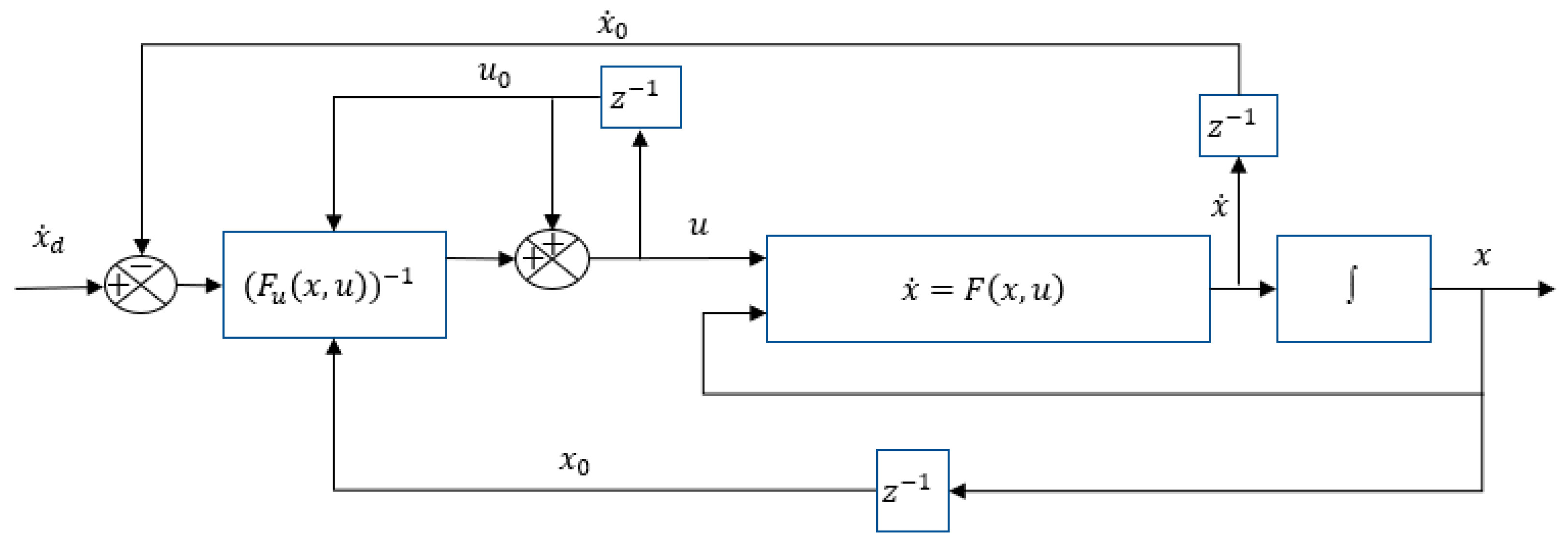
where $F_u=$($\frac{\partial F}{\partial u}{|}_{x_0,u_0}$) must be invertible and ${\dot{x}}_0, x_0$, and $u_0$ must be observable. To make sure $F_u$ is invertible in all time steps, $F_u$ must be a square matrix with a non-zero determinant. In cases when $F_u$ is not square, the pseudo inverse must be used to avoid any singularity of the controller. A block diagram of the proposed closed-loop system, as described by Equations (11)–(13), is presented in Figure 4.

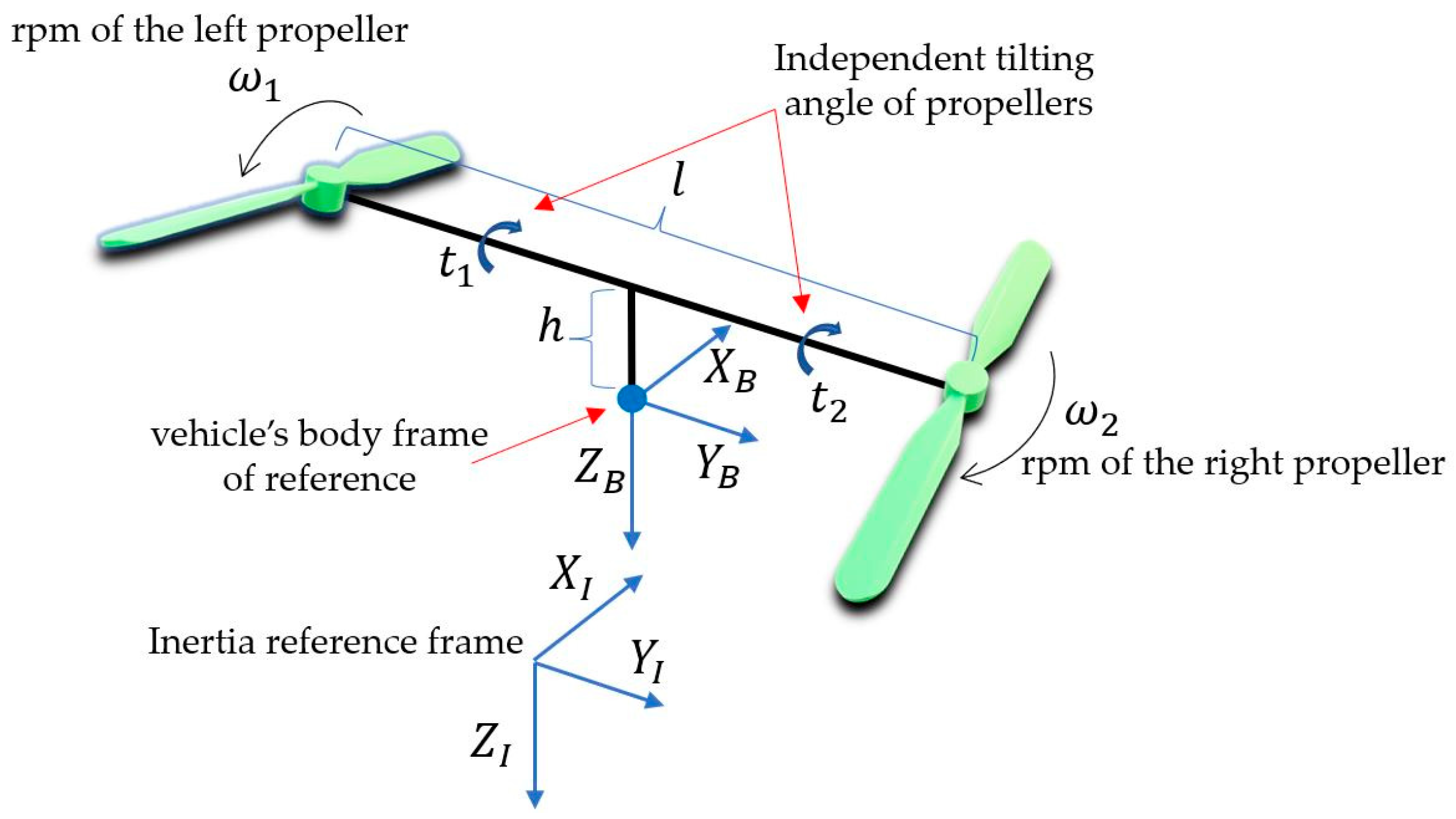
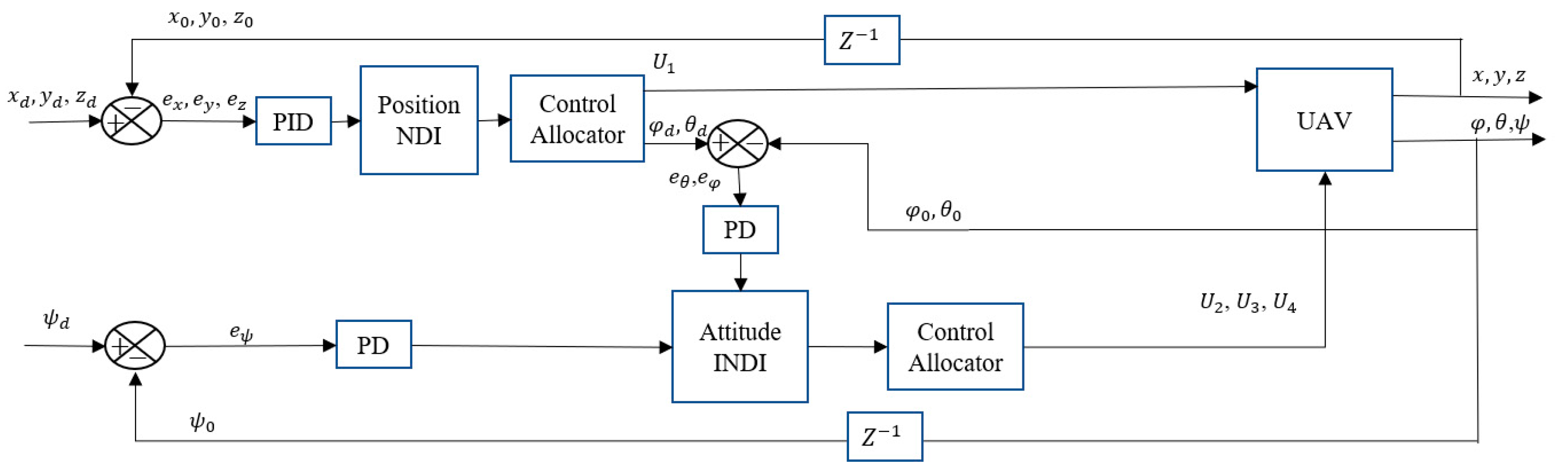
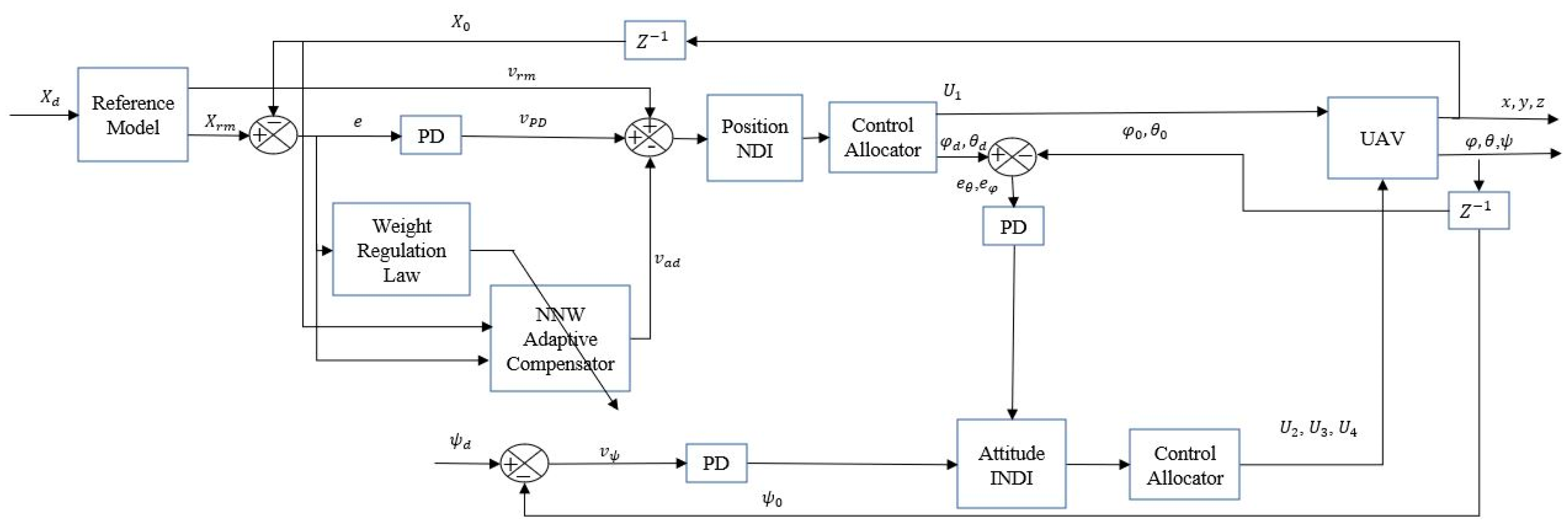
Due to the under-actuated kinematics and dynamics of the bi-copter as defined by its mathematical model (Figure 1), the timescale separation principle must be applied, dividing the control law(s) into two loops: The outer loop (designed to control the translational degrees of freedom) provides input to the inner loop (designed to control the rotational degrees of freedom). This principle is used here to ensure that the dynamics of the inner loop are fast enough so that the vehicle’s rotational motion (i.e., attitude angles and rates of change of the rotation) required by the outer loop in its computation are readily available (assumed to be immediately achieved) when needed by the slow dynamics of the outer loop. To achieve this, a nonlinear controller that combines an NDI and an INDI controller is proposed (Figure 5). The reason for this control selection is that both NDI and INDI control structures have a good ability to deal with highly coupled complex dynamic equations of the targeted UAVs and INDI provides the opportunity to use unknown/partially known dynamic equations of the aircraft in addition to being capable of dealing with other sources of uncertainties and disturbances.

Since the outer loop control has slow dynamics, an NDI controller is used for position $\left(x,y,z\right)$ control, while an INDI is used to control the aircraft’s angular rotation, $\left(\varphi ,\theta ,\psi \right)$, where faster and more complex dynamics are involved.

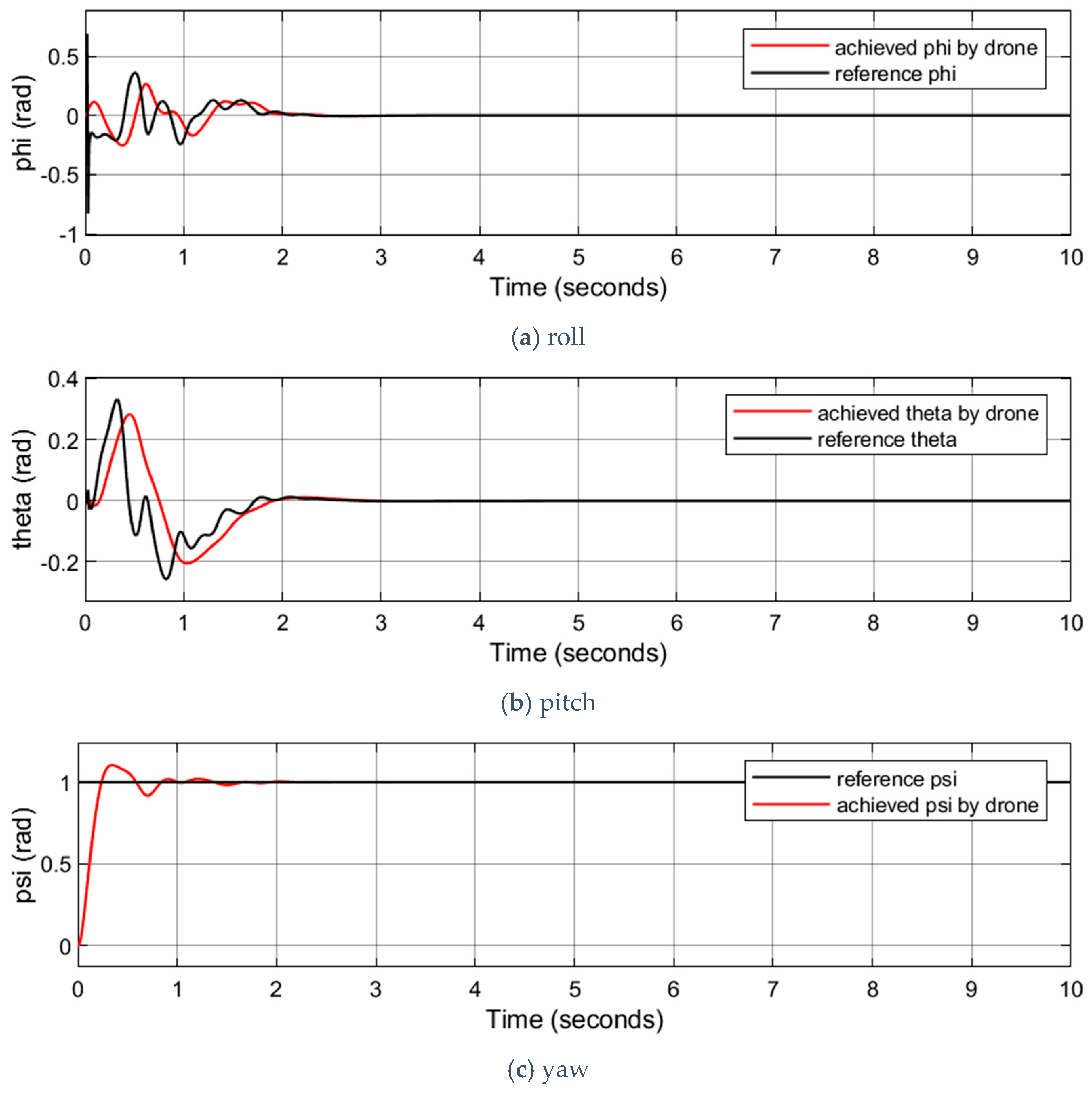
3.2. Attitude Controller

For the INDI attitude controller, the state of the drone is defined to include the Euler angles for roll, pitch, and yaw and the corresponding rotational speeds of the drone with respect to the aircraft’s body frame of reference (p, q, r), as described by Equation (14).

$$x=\left[\begin{array}{c}\vartheta \\ \omega \end{array}\right]=\left[\begin{array}{c}\varphi \\ \theta \\ \psi \\ p\\ q\\ r\end{array}\right] u=\left[\begin{array}{c}{U}_2\\ U_3\\ U_4\end{array}\right]$$

(14)

where $\vartheta =\left(\varphi , \theta ,\psi \right)$ and $\omega =\left(p, q, r\right)$. It should be noted that the mapping between $\vartheta$ and $\omega$ is defined by the corresponding transformation matrix. Since the control variables are the Euler angles, we can define $\varphi , \theta$, and $\psi$ as the output variables and later as the control variables per Equation (15).

$$\vartheta =Hx=\left[I_{3\times 3} 0_{3\times 3}\right]x$$

(15)

Since the first-order time derivative of the control variable vector, y, does not contain the control input vector, u, as described in Equations (16) and (17), the direct relationship between the input and output variables was determined by executing the second-order derivative of the control variable vector:

$$\frac{d\vartheta }{dt}=\frac{dHx}{dt}=H\dot{x}=H\left[\begin{array}{c}J\left(\vartheta \right)\omega \\ \dot{\omega }\end{array}\right]=J\left(\vartheta \right)\omega$$

(16)

$$\frac{d^2\vartheta }{d{t}^2}=\frac{d\left(J\left(\vartheta \right)\omega \right)}{dt}=\frac{d}{dx}\left(\left[\begin{array}{ccc}1& tan\theta \mathit{sin}\varphi & tan\theta \mathit{cos}\varphi \\ 0& \mathit{cos}\varphi & -\mathit{sin}\varphi \\ 0& \mathit{sin}\varphi /\mathit{cos}\theta & \mathit{cos}\varphi /\mathit{cos}\theta \end{array}\right]\left[\begin{array}{c}p\\ q\\ r\end{array}\right]\stackrel{·}{x}\right)$$

(17)

It is then clear that the input explicitly appears in the obtained expression. From this formulation, it is then possible to deduce the INDI controller for the complete system by performing a Taylor expansion in the current time step, t, as described in Equations (18) and (19). This expansion provides the linearized relationship between the control inputs and the Euler angles.

$$\ddot{\vartheta }=K_{\vartheta }\left(x,u\right)=J\left(x\right)\left[K\left(x,u\right)\right]$$

(18)

$$\ddot{\vartheta }\approx K\left(x_0, u_0\right)+\frac{\partial K_{\vartheta }\left(x,u\right)}{\partial x}{|}_{x_0,u_0}\left(x-x_0\right)+\frac{\partial K_{\vartheta }\left(x,u\right)}{\partial u}{|}_{x_0,u_0}\left(u-u_0\right)$$

(19)

The linearization shown in Equation (19) assumes $K\left(x_0,u_0\right)$ to be the angular acceleration measurement taken at the previous time step, t−1. With a very small sampling time and considering that the actuator dynamics are faster than the dynamics of the other system dynamics, it is possible to assume that $\left(x-x_0\right)\approx 0$ when compared to the changes of control output, $∆u=\left(u-u_0\right)$. When considering the high dynamics of the tiltrotor bi-copter, this assumption is quite bold. However, the dynamics of the tiltrotor bi-copter are highly dependent on the actuators’ dynamics. Even though one might think that the above-mentioned assumption (i.e., $∆T)$ leading to the assumption that the variation between samples can be considered negligible, is restrictive, in practice, such conditions can be easily met as the state changes are negligible when compared to the typical fast actuator’s dynamics available in the market, under these conditions, a simplified expression that will be later used to obtain the control law can be expressed, as shown in Equation (20):

$$\ddot{\vartheta }\simeq {\ddot{\vartheta }}_0+K\left(x_0, u_0\right)∆u$$

(20)

where matrix $K\left(x_0,u_0\right)$ is the derivative of the control inputs as shown in Equation (21).

$$K\left(x_0, u_0\right)=J\left(x_0\right)\left[\begin{array}{c}{0}_{3\times 3}\\ \begin{array}{c}\raisebox{1ex}{$l$}\!\left/ \!\raisebox{-1ex}{$I_{XX}$}\right. 0 0 \\ 0 \raisebox{1ex}{$h$}\!\left/ \!\raisebox{-1ex}{$I_{YY}$}\right. 0\\ 0 0 \raisebox{1ex}{$l$}\!\left/ \!\raisebox{-1ex}{$I_{ZZ} $}\right.\end{array}\end{array}\right]$$

(21)

$$∆u=K{\left(x_0, u_0\right)}^{-1}\left(\ddot{\vartheta }-{\ddot{\vartheta }}_0\right)$$

(22)

Using Equation (20), as the control law, one can then obtain the input for the system by considering a simple relationship $∆u=\left(u-u_0\right)$, where $u_0$ is the previous input, and solving Equation (22) to reach the control input $u.$ The formulation $K{\left(x_0, u_0\right)}^{-1}$ can then be used to calculate the needed control input at each time step where, based on the previous assumptions, the system will not enter singularity points in the cases where K is not invertible (as the pseudo inverse can be computed in such cases, enabling the controller to pass such conditions).

The nonlinear controller obtained in this form is slightly less dependent on the system’s mathematical model, thus enabling it to effectively obtain the control input base on the angular acceleration measurements, which, otherwise, would be challenging to obtain. Even though the controller does not depend on part of the model, it is verifiable that the part of the controller that is neglected only slightly influences the bi-copter’s behavior. Therefore, disregarding the slower dynamics of the model when the controller is designed does not significantly affect the bi-copter’s behavior.

3.3. Position Controller

As described above, to control the position of the UAV, an NDI controller is used comprising the outer loop within the proposed controller (Figure 5).

The proposed position controller follows a similar approach as the one developed for attitude control. The first control layer uses the INDI technique to cancel the nonlinearities associated with the linear dynamics of the system. Since, in the approach illustrated in Figure 5, the outer loop is less dependent on the model uncertainty, NDI can be effectively used to design the corresponding position controller. The virtual control variables, u, chosen for this controller are defined as per Equation (23).

$$u=\left[\begin{array}{c}{U}_x\\ U_y\\ U_z\end{array}\right]=\left[\begin{array}{c}{U}_1\left(sin\varphi sin\psi +cos\varphi sin\theta cos\psi \right)\\ U_1\left(-sin\varphi cos\psi +cos\varphi sin\theta sin\psi \right)\\ U_1 cos\varphi cos\theta \end{array}\right]$$

(23)

Therefore, based on the equations presented in Section 3.1, the first-order time derivative of y for the NDI position controller is given per Equation (24).

$$\dot{X}=f\left(x\right)+G\left(x,u\right)u$$

(24)

Since an explicit dependence on u was already found (i.e., Equation (22)), the linear relationship $\mathsf{\upsilon }=\dot{\mathrm{X}}$ can then be imposed when det $G\left(x,u\right)\ne 0$ by selecting the control input vector, u, have the form described by Equation (25).

$$u=G{\left(x,u\right)}^{-1}\left(\upsilon -f\left(x\right)\right)$$

(25)

As in Section 3.2, it is common to use a PID controller to improve the response of the system. For this, however, there is a need to obtain the optimized values of the PID gains. To obtain such gains in the scope of the multi-objective goal for the bi-copter UAV, a non-dominated sorting algorithm, NSGA-II, is used (described in Section 4).

The NDI outer loop controls the slow dynamics and generates the state command to the inner INDI block following Equations (26)–(28), as is shown in Figure 5.

$${\theta }_d=ta{n}^{-1}\left(\frac{U_{x}cos\psi +U_{y}sin\psi }{U_z}\right)$$

(26)

$${\varphi }_d=ta{n}^{-1}\left(\frac{cos{\theta }_d\left(U_{x}sin\psi -U_{y}cos\psi \right)}{U_z}\right)$$

(27)

$$U_1=\frac{U_z}{cos{\theta }_{d}cos{\varphi }_d}$$

(28)

4. NSGA-II

In general terms, the NSGA-II technique is a well-known fast sorting and selection multi-objective genetic algorithm. This algorithm is typically used in machining to select diverse process parameters such as cutting speed, spindle rotational speed, and feed rate [36] needed to optimize the corresponding machining operation.

In this paper, NSGA-II is used to optimize the parameters of the PID controller shown in Figure 5, which provide the inputs to the NDI and INDI controllers described in Section 3, where the number of parameters is large, and an analytical solution is difficult to obtain. More specifically, we aim to tune the linear controller gains as an essential part of obtaining an accurate controller. Therefore, in this paper, the non-dominated sorting-based multi-objective evolutionary algorithm (MOEA), called the non-dominated sorting genetic algorithm II (NSGA-II), is used. By using this method, the goal is to optimize the PID linear parameter, which has a significant role in the behavior of the desired controller. During the optimization process, two different objectives are considered: the integral of the time-weighted absolute error (ITAE) performance index and the integral of the square of the error (ISE). Whereas minimizing the first objective will provide good reference tracking and good disturbance rejection, minimizing the second reduces the rise time. The mathematical descriptions of these two objectives are given by Equations (29) and (30), respectively:

$$O{b}_1=ITAE={\int }_0^{T_s}t|e\left(t\right)|dt$$

(29)

$$O{b}_2=ISE={\int }_0^{T_s}e{\left(t\right)}^{2}dt$$

(30)

where the error signal e(t) is defined as the difference between the reference input signal and the controlled variable, and $T_s$ is the simulation time.

5. Simulation Results

In order to analyze the advantages and disadvantages of the proposed control algorithm, as well as to quantify the differences with and without the gain optimization process, two sets of simulation results are presented (Section 5.1 and Section 5.2, respectively).

Table 1. Parameters of the bi-copter UAV.

Mass (kg)	Length (m)	Height (m)	Propeller Tilt Angle Range
			t1 (Rad)	t2 (Rad)
0.87	0.23	0.1	±0.26	±0.26
Ixx (N·m2)	Iyy (N·m2)	Izz (N·m2)	IXZ (N·m2)	Max ω1&2 (rpm)
0.04	0.04	0.04	0.01	7650

provides the values of the parameters that describe the bi-copter UAV and were used to obtain the results described in Section 5.1 and Section 5.2.

5.1. Simulation before Optimization

As an example of the numerous tests performed when controlling the UAV without gain parameter optimization, the UAV was commanded to track the trajectory shown in Figure 6, following a circular path defined by a set of x, y, and z points represented in Equation (31). It should be mentioned that $x, y, z$, and $\psi$ are the controllable states, and the desired values of $\varphi$ and $\theta$ are computed in the control allocation block to enable the system to follow the desired trajectory.

$$\begin{gathered} x=\mathit{sin}\left(0.05t\right) \\ y=-\mathit{cos}\left(0.05t\right) \\ z=1 \end{gathered}$$

(31)

At the start of the simulation, the UAV is located at the takeoff site where the UAV is positioned 1 unit distance from the height where the desired circular trajectory is to be followed (see Figure 6). At takeoff, the UAV rapidly climbs to reach the required altitude. Since there is no constraint on how the vehicle intercepts the given flight path, how the aircraft reaches the desired trajectory (e.g., speed of climb) is entirely governed by the proposed INDI + NDI + PID controller.

During the test, the PD and PID gains are represented by a 1 × 18 vector, the elements of which correspond to the P and D gains of the corresponding controllers for the $\varphi ,\theta ,$ and $\psi$ angles (nine gains, considering the corresponding I gains are equal to zero), and the P, I, and D gains for the position $x,y,$ and $z$ (nine gains) for a total of 18 preselected values as shown in the following k vector (k = [k_P^φ, k_I^φ, k_D^φ; k_P^θ, k_I^θ, k_D^θ; k_P^ψ, k_I^ψ, k_D^ψ; k_P^x, k_I^x, k_D^x; k_P^y, k_I^y, k_D^y; k_P^z, k_I^z, k_D^z]):

$$k=\left[2.5 , 0 , 10 , 2.5 , 0 , 10 , 2.5 , 0 , 10 , 1 , 0 , 3 , 1 , 0 , 3 , 5 , 1 , 10\right]$$

(32)

These 18 gains were selected by trial and error, which were considered the best set of gains. Since the response of the propellers’ rotation angles and the position response of the UAV in the z-direction occurs very fast, the UAV reaches the desired height rapidly, and subsequently, it becomes more evident how the controller guides the UAV to follow the x and y values of the desired trajectory. Figure 7 and Figure 8 show the results for the position and orientation when the UAV was under control using non-optimal gains (Equation (32)).

5.2. Simulation after Optimization

Similar to the test presented in Section 5.1, a second simulation test was performed using the aspects described in Section 5.1 (e.g., same UAV parameters, same takeoff position, and same desired trajectory) but using an optimized set of gains. The purpose is to compare and show the effects of the optimization process on the system’s behavior. To obtain the optimal set of gains, the NSGA-II optimization technique described in Section 4 was used to minimize the two objective functions, $O{b}_1$ and $O{b}_2$, defined by Equations (29) and (30). To perform such optimization, a population size equal to 30 was used while the optimization cycle was repeated for 100 generations., During the optimization process, crossover and mutation rates equal to 0.95 and 0.01, respectively, were used. The parameters (gains) optimized in this process included $K_P,K_I,\mathrm{and}{K}_D$ for each of the x, y, z,$\varphi ,\theta$ and $\psi$ parameters (18 gains in total), respectively (note that in this case, the integral gains for the three angular orientations were considered as zero). The range of decision variables for $K_P,K_D$ was selected to be between 0 and 15, while the range for the gains $K_I$ were selected to be between 0 and 1. This variable range selection was based on numerous simulation results used to eliminate reaching singularity points. The result of the optimization process produced the following k vector.

$$k=\left[10.6,0,13.4,0,5.8,0,8.8,10.8,13.0,4.3,1.9,3.6,6,0,3.5,8.4,0.2,8\right]$$

Figure 9 shows the changes in the optimization cost functions before and after the optimization process for each state. Figure 9 shows the significant changes that took place in the objective functions for all states.

Figure 10, Figure 11 and Figure 12 present the simulation result for position and orientation to track the desired trajectory and illustrate the obtained trajectory that the UAV generated. When compared to the first test (Section 5.1), the results using the optimized gains show faster trajectory tracking and, thus, better UAV performance. This is especially true in position tracking where the UAV converges to the desired path much faster and uses a smoother path.

Figure 10 and Figure 11 illustrate the effect of the optimization on the controller results. Not only were the steady-state errors of all state variables reduced, but the average overshoot of the corresponding responses and the settling time of the system also showed significant improvements.

5.3. Wind Gust Disturbances

To show the effectiveness of the proposed controller to identify and control the aircraft under external disturbances, the drone was tested under diverse wind gust conditions showing the robustness of the proposed control mechanisms. To test such aspects, the tiltrotor bi-copter drone shown in Figure 1 was flown within an uncertain outdoor flying environment simulation. Within such a simulation environment, the aircraft was placed under moderate wind disturbances mimicking real wind conditions. Although the wind effect is typically considered a constant within the available literature (as it is very challenging to simulate the variability of real-world wind conditions), such wind effects do not reflect real flight conditions, and as a result, it leads to misleading conclusions about the performance of the tested control scheme. In contrast to such simplistic approaches, in this paper, the control scheme described in the previous sections was tested using a macro approach, which defines two main characteristics of typical wind: the magnitude and the direction of the wind velocity. To define the wind affecting the aircraft during the simulation tests, the description and wind formulations used in [37] were employed. Thus, in the tests conducted, the azimuth ${\psi }_w$ of the point from which the wind blows was used as a wind direction, where a random value $∆{\psi }_w$ was use to represent the random value of wind direction change. The azimuth is measured from the north point through the east. The velocity of the wind is also defined as a function of the z (altitude) position of the UAV (drone), $V_z$ with respect to the sea level. Based on the results provided in [37], a moderate horizontal wind gust of 4 m/s was used to study the stability and robustness of the designed controller. The following formula was used to determine the average wind velocity as a function of the drone’s altitude:

$$V_z=V_{z_0}{\left(\frac{z}{z_0}\right)}^p$$

where $V_z$ is the wind velocity at altitude z, $V_{z_0}$ is the specified (measured) wind velocity at altitude $z_0$, and p is the index of the energetic wind profile. This formulation was used to compute the wind that the drone would experience as it changes altitude while tracking the desired trajectory. Furthermore, to better simulate the wind disturbances that the tiltrotor bi-copter drone would experience, the wind force that influences the aircraft was considered to be more representative than the actual instantaneous wind velocity. To compute such a force, the following formulation was used

$$F_w=S_{e}A{V}_z{}^2$$

where $S_e$ is the influence effective area, and A = 1/16 × 9.81 = 0.61 is the rate of wind velocity ($\mathrm{m}/{\mathrm{s}}^2$) conversion to pressure ($\mathrm{N}/{\mathrm{m}}^2$). To compute the total force and its distribution over the drone’s fuselage, the tiltrotor bi-copter was represented as a cylindrical body. Even though this is a very simplistic approximation, it enabled us to test the robustness of the controller to external a priori unknown wind disturbances. The expression determining the bi-copter surface area was set to be equal to the sum of the lateral surface area, $S_l$, and the area of the base, $S_b$, as represented by the following mathematical expression where r and h are the radius and height of the cylinder representing the drone, and a and b are the fill factors of the cylinder area that depend on the tiltrotor bi-copter design.

$$S=S_l+S_b=a2\pi rh+b2\pi r^2$$

5.3.1. Nonlinear Dynamic Inversion Structure with Neural Network Augmentation

Because of the sensitivity of the dynamic inversion approach to the accuracy of the dynamic model, a sigma-pi neural network (NN) adaptive compensator is used to compensate for modeling errors [38]. Thus, the control scheme shown in Figure 5 is enhanced to include a NN adaptive compensator, as illustrated in Figure 13. The modeling error feeds the NN, which, in turn, generates an output to compensate for deviations due to the approximate NDI output. It is important to note that such NN is applied to each of the channels (x, y, and z), where each NN might have different weights.

Considering the model error, the new model of the system can be defined as Equation (33):

$$\ddot{x}=\widehat{f}\left(x,\dot{x},u\right)+∆\left(x,\dot{x},u\right)$$

(33)

where $∆\left(x,\dot{x},u\right)=\ddot{x}-\widehat{f}\left(x,\dot{x},u\right)$ represents the model inversion error. The sigma-pi NN compensates the inversion error adaptively with a real-time pseudo control signal $v_{ad}$ where the pseudo control command is provided as per Equation (34):

$$v=v_{rm}+v_{pd}-v_{ad}$$

(34)

where $v_{rm}=$ $\ddot{x}$ is the reference model’s pseudo control, and $v_{pd}$ is the PD linear regulator used to regulate the dynamic response of the system as per Equation (35):

$$v_{pd}=k_p\left(x_{rm}-x\right)+k_d\left({\dot{x}}_{rm}-\dot{x}\right)$$

(35)

As a result, the dynamics of the model tracking error can then be described via Equation (36):

$$\dot{e}=Ae+B\left(v_{ad}-∆\right)$$

(36)

where $e=\left[\begin{array}{c}{x}_{rm}-x\\ {\dot{x}}_{rm}-\dot{x}\end{array}\right],A=\left[\begin{array}{c}0 1\\ -k_p-k_d\end{array}\right]$, and B = $\left[\begin{array}{c}0\\ 1\end{array}\right].$

5.3.2. Neural Network Design

The sigma-pi neural network (NN) acting as the adaptive compensator shown in Figure 13 can be made up of any linearly parameterized feedforward structure capable of reconstructing the inversion error, as depicted in Figure 14.

The neural network’s input/output map can be represented as follows:

$$v_{ad}={\displaystyle \sum }_{j=1}^k{w}_j{\beta }_j\left(\overline{X},\nu \right)=W^T\beta \left(\overline{X},\nu \right)$$

(37)

where $\overline{X}$ represents the normalized states, $W$ is a vector of variable networks weights, and $\beta \left(c_1,c_2,c_3\right)=kron\left(kron\left(c_1,c_2\right),c_3\right)$ is a network basis function vector. The corresponding weight error can then be described as follows (Equation (38)):

$$\tilde{W}=W-W^{*}$$

(38)

where $W^{*}$ denotes the ideal set of weights. Thus, the error vector can be written as per Equation (39), and the updated law for the NN can be expressed by Equation (40).

$$\dot{e}=Ae+B{\tilde{W}}^T\beta +B\left(W^{*}{}^T\beta -∆\right)$$

(39)

$${\dot{\tilde{W}}}_i\left(t\right)=\{\begin{array}{c}-{\Gamma }_i\left(e^T{}_i{P}_{i}B\right){\beta }_i for \Vert e_i\Vert {}_{P_i}>e_{0_i}\\ 0 for \Vert e_i\Vert {}_{P_i}<e_{0_i}\end{array} , i=1,2,\dots ,n$$

(40)

where $\Vert e_i\Vert {}_{P_i}=\sqrt{e^T{}_i{P}_i{e}_i}$, ${\Gamma }_i$ is a positive constant adaptation gain (learning rate), and $P_i$ is a symmetric, positive definite matrix satisfying the Lyapunov equation $P_i{A}_i+A_i{}^T{P}_i=-I$ for the linear system error with NN weights. The Hurwitz matrix $A_i$ of Equation (38) ensures the existence of a unique $P_i=P_i^T>0$ where $P_i$ is described as per Equation (41):

$$P_i=\left[\begin{array}{c}\frac{K_{d_i}}{2K_{p_i}}+\frac{K_{p_i}}{2K_{d_i}}\left(1+\frac{1}{K_{p_i}}\right) \frac{1}{2K_{p_i}}\\ \frac{1}{2K_{p_i}} \frac{1}{2K_{d_i}}\left(1+\frac{1}{K_{p_i}}\right)\end{array} \right]$$

(41)

Figure 15 shows one of the many wind profiles used when testing the proposed controller. Under such wind conditions, the aircraft was commanded to take off and fly following the trajectory defined by the desired x, y, and z curves shown in Figure 16. Figure 16 also shows the drone’s position in terms of the flight path achieved by the drone and its deviation from its intended path.

6. Conclusions

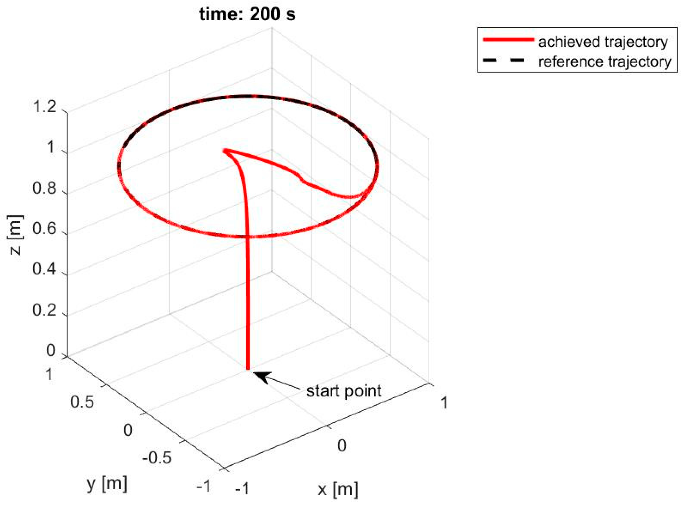
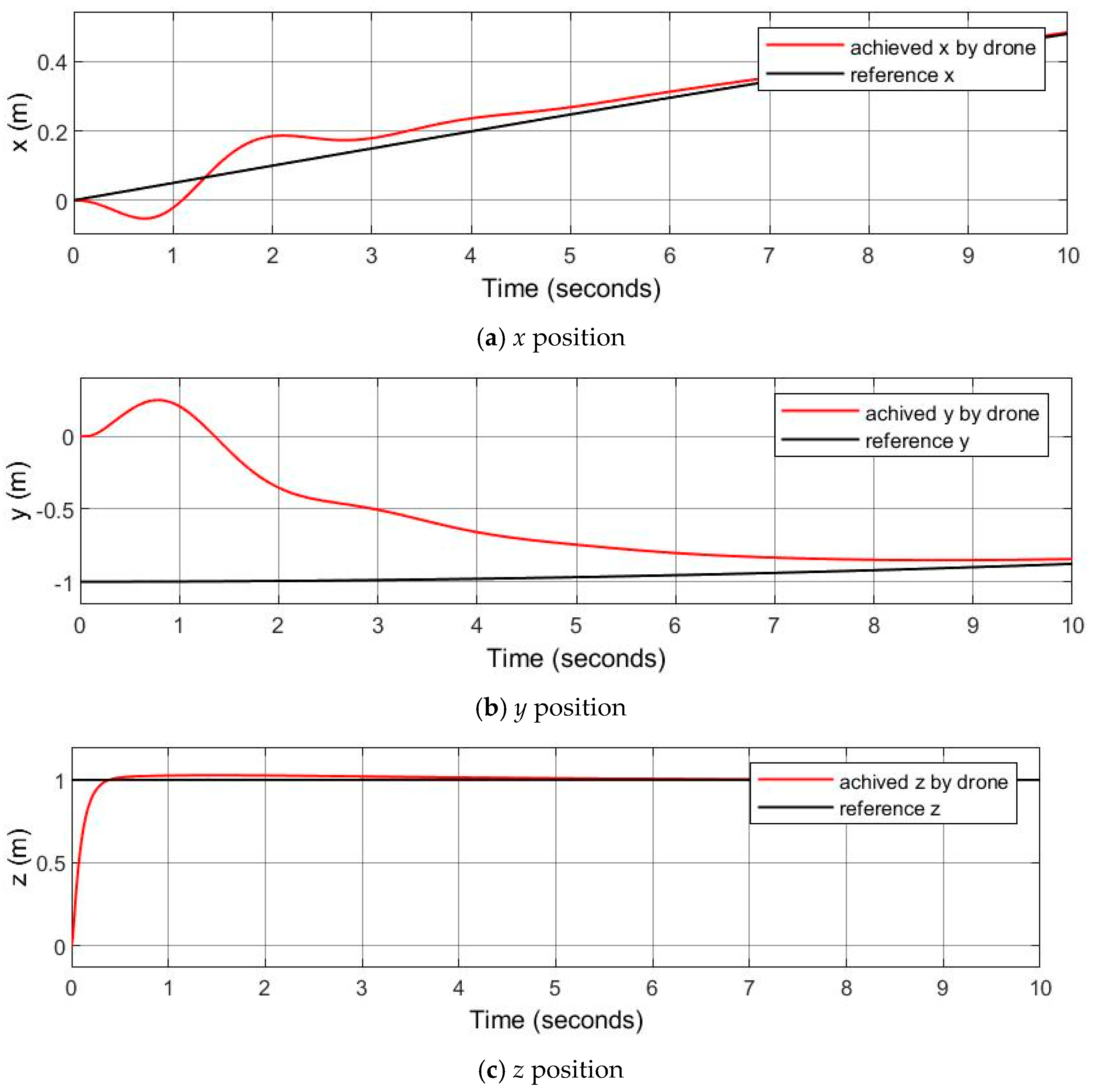
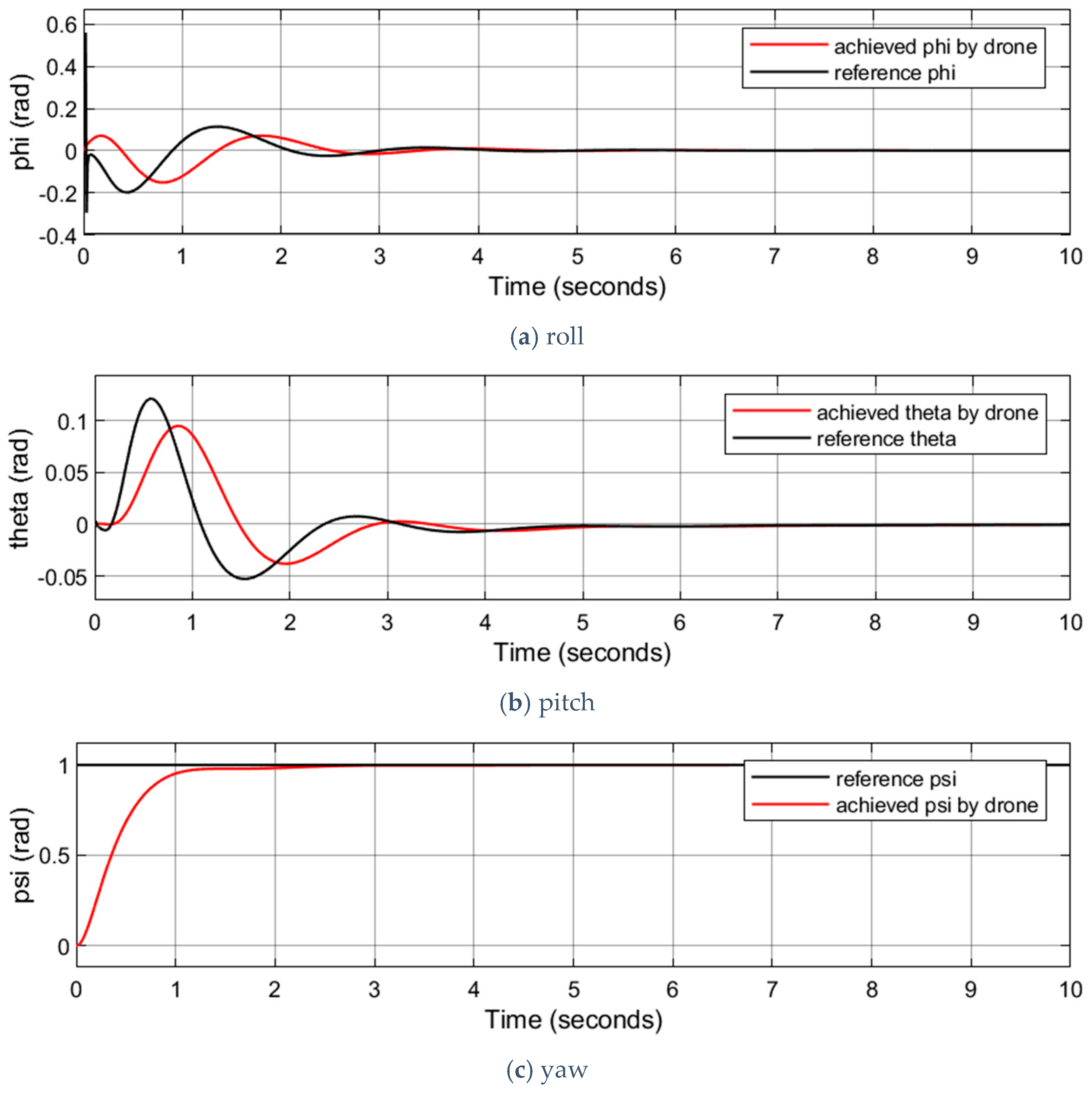
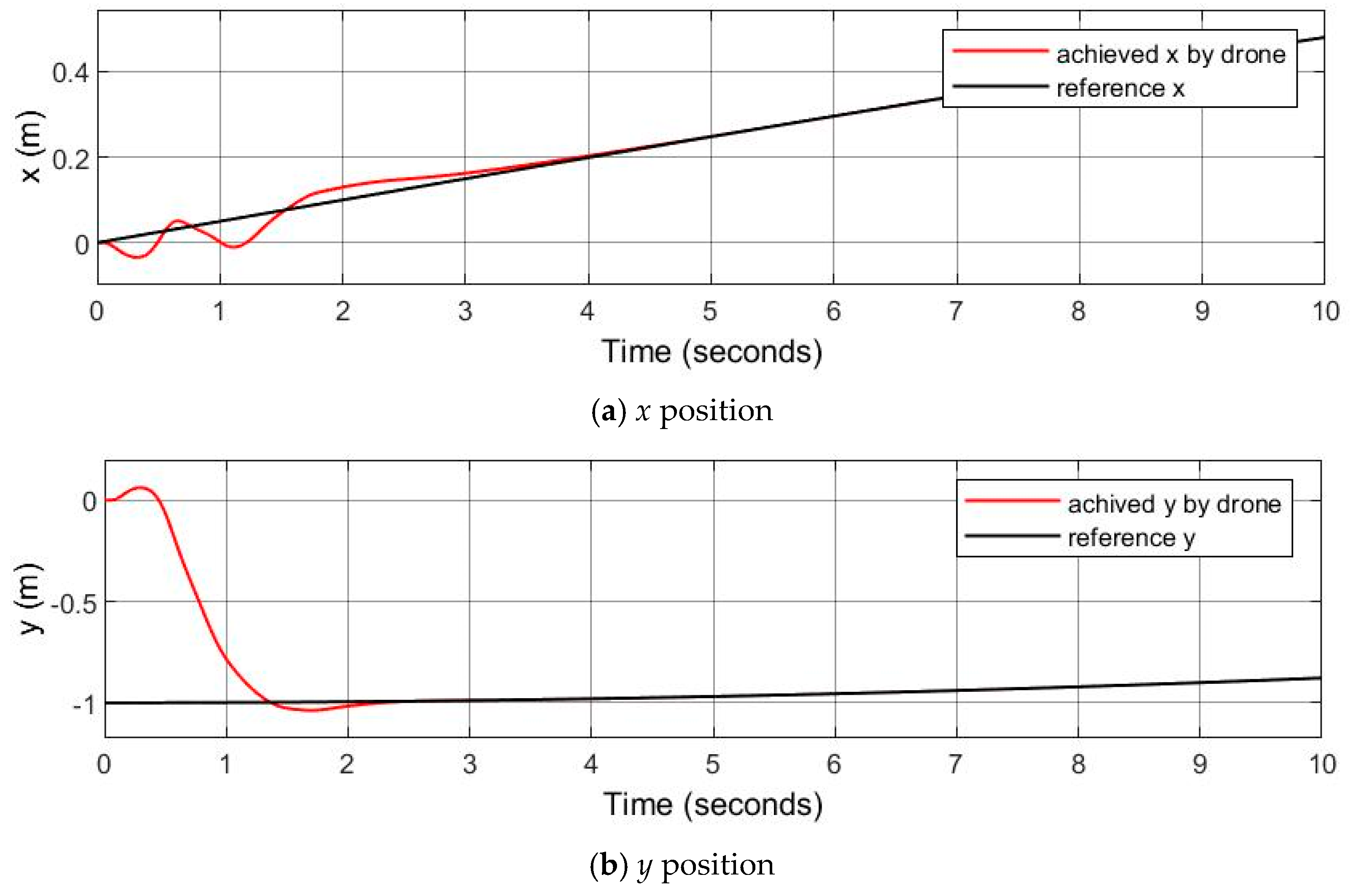
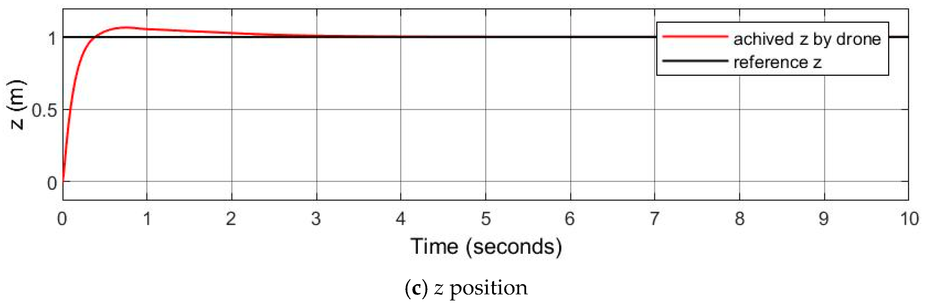
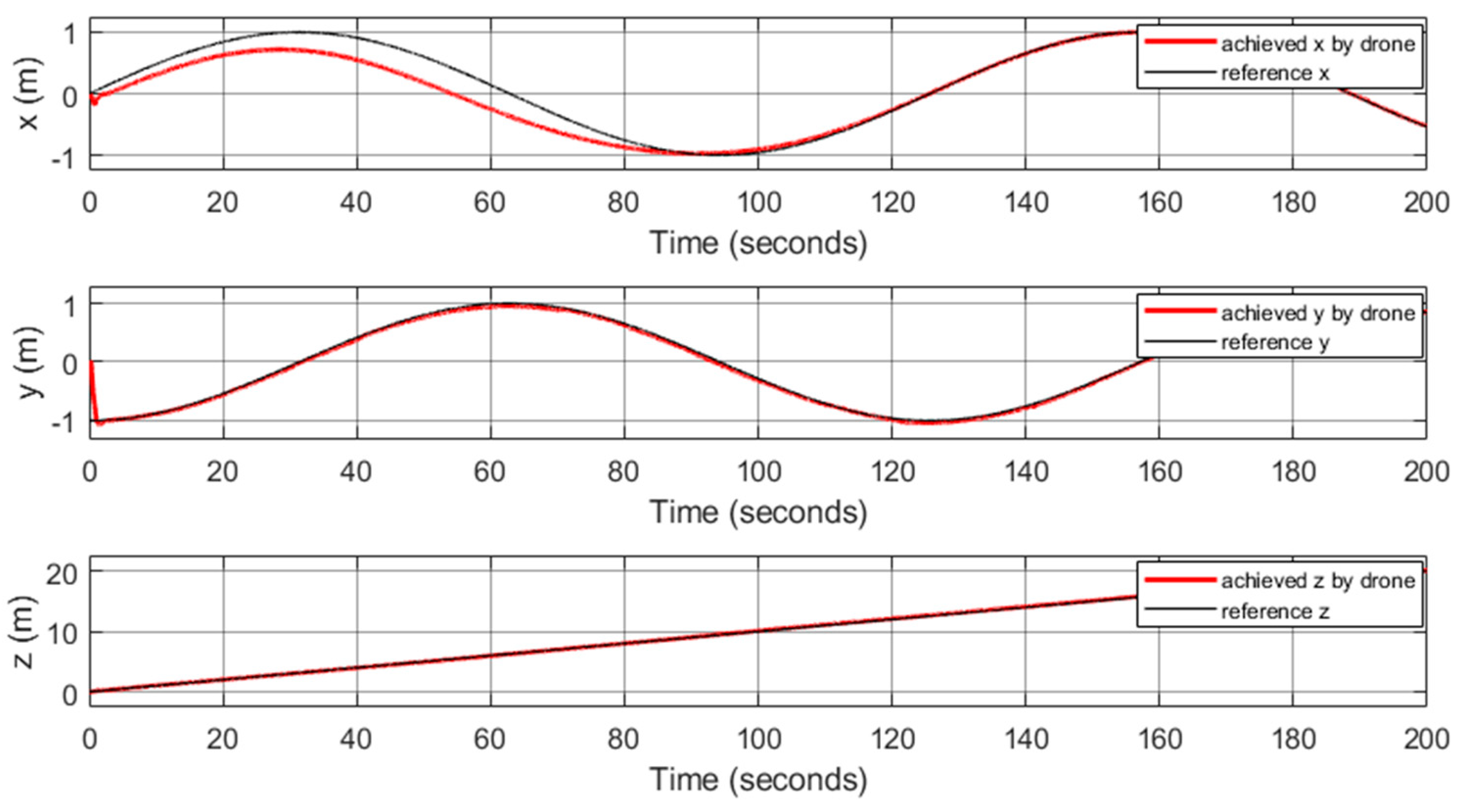
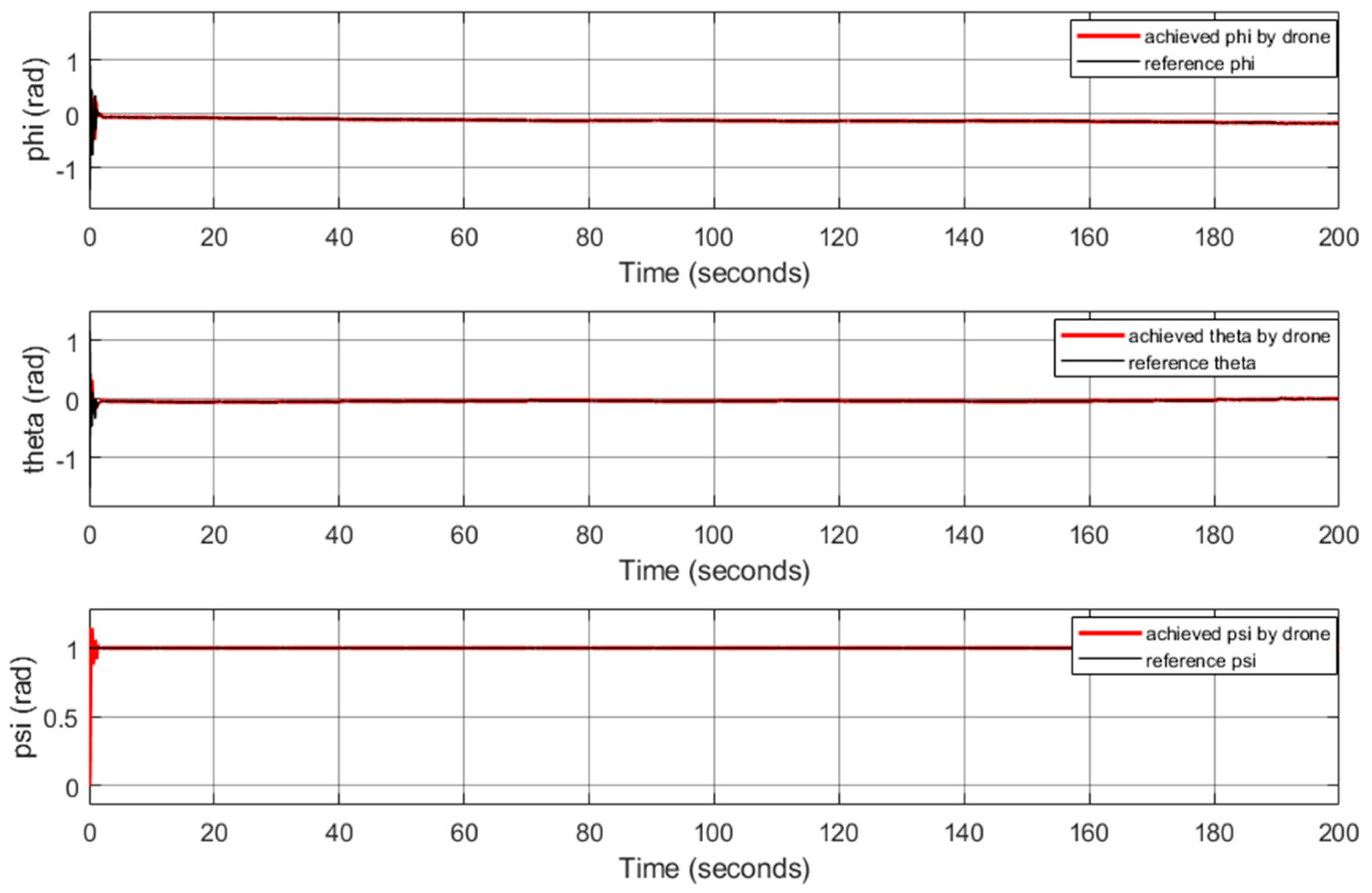
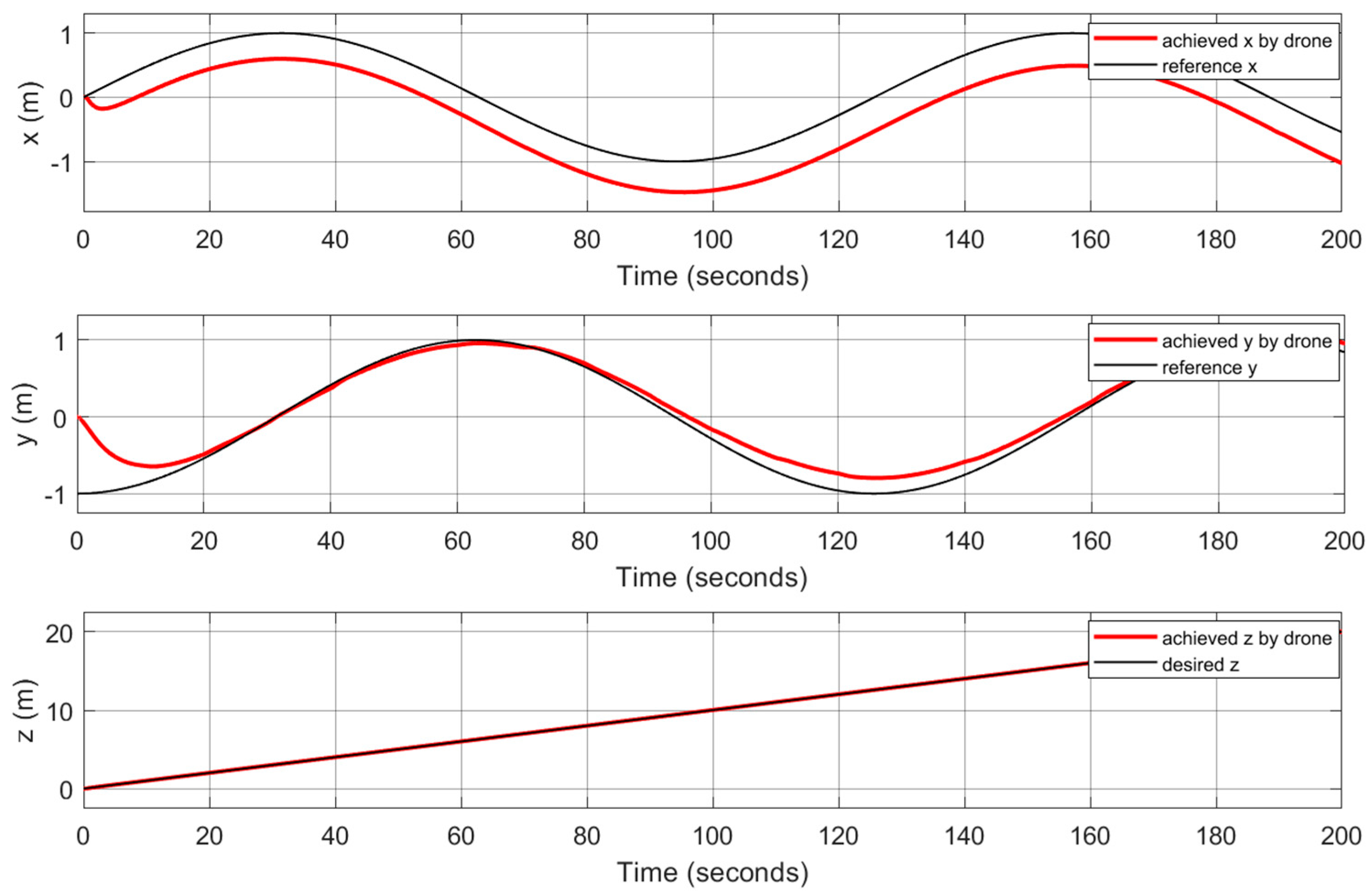
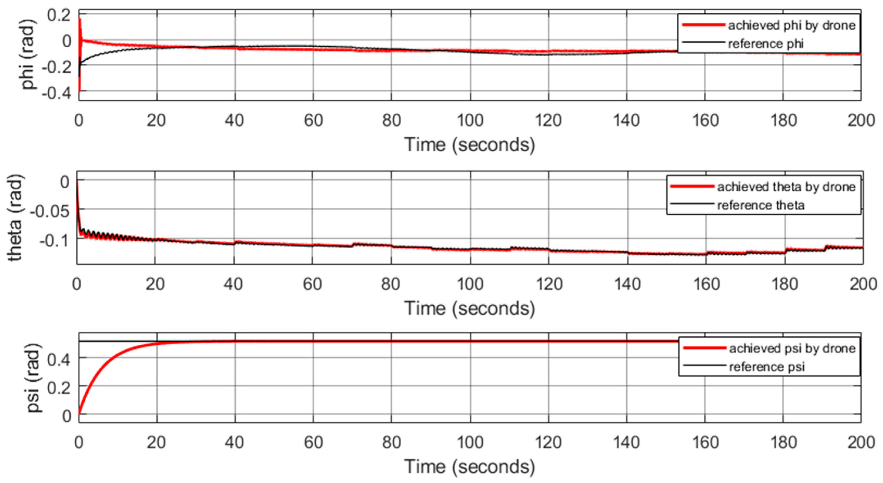
In this paper, a nonlinear mathematical model for a tiltrotor bi-copter UAV prototype is extracted. Then, a nonlinear trajectory controller based on nonlinear dynamic inversion, including an outer NDI loop controller for position and an inner INDI loop controller for orientation is proposed. The proposed control architecture is improved with the introduction of the NSGA-II-PID controller. Due to the significant cost in time and effort required to repetitively perform manual tuning of the linear gains using typical control tunning approaches, in this paper, a multi-objective-gain optimization process based on the NSGA-II algorithm is used to minimize the two error functions. By combining these two controllers with a multi-objective optimization process, faster and more accurate flight control is achieved. The proposed controller does not require a complete and accurate dynamic model of the system. The performance of the control system was tested over diverse flight paths, including flight tests under moderate wind gusts.

The obtained results of the proposed controller, implementing gain matrix k = [10.6, 0, 13.9, 5.8, 0, 8.8, 10.8, 0, 13.0, 4.3, 0, 3.6, 6, 0, 3.5, 8.4, 0, 8] for the PID control blocks, were compared with results obtained using a previously designed backstepping controller, using a gain matrix α equal to α = [15, 0.1, 15, 0.1, 15, 0.1, 20, 1, 2, 1, 1, 1]. From the obtained results, it is concluded that the proposed control system design performs better than previously developed controllers (e.g., the backstepping controller, which requires accurate equations of motion) and provides better results than the classic dynamic inversion type of controllers presented in the available literature. These results are anticipated to be very helpful for the development of a new concept of bi-copter aircraft using diverse mechanisms, including variable pitch propeller systems and other architectures that will enable such eVTOL aircraft to perform missions in civil and military applications and overcome aggressive disturbances where current UAV systems cannot be used.

As described in this paper, the proposed method is an offline method. However, it could be used online if the needed time window for optimization is calculated and guaranteed prior to the actual flight.

References

1. Ramanathan, V.; Ramana, M.; Roberts, G.; Kim, D.; Corrigan, C.; Chung, C.; Winker, D. Warming trends in Asia amplified by brown cloud solar absorption. Nature 2007, 448, 575–578. [Google Scholar] [CrossRef] [PubMed]
2. Alotaibi, E.T.; Alqefari, S.S.; Koubaa, A. Lsar: Multi-uav collaboration for search and rescue missions. IEEE Access 2019, 7, 55817–55832. [Google Scholar] [CrossRef]
3. Sarghini, F.; De Vivo, A. Analysis of preliminary design requirements of a heavy lift multirotor drone for agricultural use. Chem. Eng. Trans. 2017, 58, 625–630. [Google Scholar]
4. Tsouros, D.C.; Bibi, S.; Sarigiannidis, P.G. A review on UAV-based applications for precision agriculture. Information 2019, 10, 349. [Google Scholar] [CrossRef]
5. Anuj, P. A Survey of Unmanned Aerial Vehicles (UAV) for Traffic Surveillance; University of South Florida: Tampa, FL, USA, 2005; pp. 1–29. [Google Scholar]
6. Puttock, A.K.; Cunliffe, A.M.; Anderson, K.; Brazier, R.E. Aerial photography collected with a multirotor drone reveals impact of Euraian beaver reintroduction on ecosystem structure. J. Unmanned Vehicle Syst. 2015, 3, 123–130. [Google Scholar] [CrossRef]
7. Chen, H.; Lan, Y.; Fritz, B.K.; Hoffmann, W.C.; Liu, S. Review of agricultural spraying technologies for plant protection using unmanned aerial vehicle (UAV). Int. J. Agric. Biol. Eng. 2021, 14, 38–49. [Google Scholar] [CrossRef]
8. Zhang, Q.; Liu, Z.; Zhao, J.; Zhang, S. Modeling and attitude control of Bi-copter. In Proceedings of the 2016 IEEE International Conference on Aircraft Utility Systems (AUS), Beijing, China, 10–12 October 2016; IEEE: New York, NY, USA, 2016; pp. 172–176. [Google Scholar]
9. Jansen, F. Manoeuvring Unmanned Vehicles through Confined 3D Environments Using Model Predictive Control. Master’s Thesis, University of Calgary, Calgary, AB, Canada, 2011. [Google Scholar]
10. Amiri, N.; Ramirez-Serrano, A.; Davies, R.J. Integral backstepping control of an unconventional dual-fan unmanned aerial vehicle. J. Intell. Robot. Syst. 2013, 69, 147–159. [Google Scholar] [CrossRef]
11. Bagheri, P.; Ramirez-Serrano, A.; Pieper, J.K. Adaptive nonlinear robust control of a novel unconventional unmanned aerial vehicle. Control Intell. Syst. 2015, 43, 274–280. [Google Scholar] [CrossRef]
12. Kamal, A.M.; Ramirez-Serrano, A. Systematic methodology for aircraft concept development with application to transitional aircraft. J. Aircraft 2020, 57, 179–197. [Google Scholar] [CrossRef]
13. Abedini, A.; Bataleblu, A.A.; Roshanian, J. Robust Backstepping Control of Position and Attitude for a Bi-copter Drone. In Proceedings of the 2021 9th RSI International Conference on Robotics and Mechatronics (ICRoM), Tehran, Iran, 17–19 November 2021. [Google Scholar]
14. Albayrak, Ö.B.; Ersan, Y.; Bağbaşı, A.S.; Başaranoğlu, A.T.; Arıkan, K.B. Design of a Robotic Bicopter. In Proceedings of the 2019 7th International Conference on Control, Mechatronics and Automation (ICCMA), Delft, The Netherlands, 6–8 November 2019. [Google Scholar]
15. Qin, Y.; Xu, W.; Lee, A.; Zhang, F. Gemini: A compact yet efficient bi-copter uav for indoor applications. IEEE Robot. Autom. Lett. 2020, 5, 3213–3220. [Google Scholar] [CrossRef]
16. Li, Y.; Qin, Y.; Xu, W.; Zhang, F. Modeling, identification, and control of non-minimum phase dynamics of bi-copter uavs. In Proceedings of the 2020 IEEE/ASME International Conference on Advanced Intelligent Mechatronics (AIM), Boston, MA, USA, 6–9 July 2020. [Google Scholar]
17. Martins, L.; Cardeira, C.; Oliveira, P. Feedback linearization with zero dynamics stabilization for quadrotor control. J. Intell. Robot. Syst. 2021, 101, 1–17. [Google Scholar] [CrossRef]
18. Das, A.; Lewis, F.; Subbarao, K. Backstepping approach for controlling a quadrotor using Lagrange form dynamics. J. Intell. Robot. Syst. 2009, 56, 127–151. [Google Scholar] [CrossRef]
19. Kurum, I. Urban Design in City and Regional Planning. Master’s Thesis, Middle East Technical University, Ankara, Turkey, 2019. Available online: https://etd.lib.metu.edu.tr/upload/12624222/index.pdf (accessed on 9 September 2019).
20. Pereira, J.C.; Leite, V.J.; Raffo, G.V. Nonlinear Model Predictive Control on SE (3) for Quadrotor Aggressive Maneuvers. J. Intell. Robot. Syst. 2021, 101, 1–15. [Google Scholar] [CrossRef]
21. Altan, A.; Hacıoğlu, R. Model predictive control of three-axis gimbal system mounted on UAV for real-time target tracking under external disturbances. Mech. Syst. Signal Process. 2020, 138, 106548. [Google Scholar] [CrossRef]
22. González, I.; Salazar, S.; Lozano, R. Chattering-free sliding mode altitude control for a quad-rotor aircraft: Real-time application. J. Intell. Robot. Syst. 2014, 73, 137–155. [Google Scholar] [CrossRef]
23. Tripathi, V.K.; Kamath, A.K.; Verma, N.K.; Behera, L. Fast terminal sliding mode super twisting controller for position and altitude tracking of the quadrotor. In Proceedings of the International Conference on Robotics and Automation (ICRA), Montreal, QC, Canada, 20–24 May 2019; pp. 6468–6474. [Google Scholar]
24. Hadi, R.; Afshinfar, S. Neural network-based adaptive sliding mode control design for position and attitude control of a quadrotor UAV. Aerosp. Sci. Technol. 2019, 91, 12–27. [Google Scholar]
25. Zhou, Q.L.; Zhang, Y.; Rabbath, C.A.; Theilliol, D. Design of feedback linearization control and reconfigurable control allocation with application to a quadrotor UAV. In Proceedings of the 2010 Conference on Control and Fault-Tolerant Systems (SysTol), Nice, France, 6–8 October 2010. [Google Scholar]
26. Smith, P. A simplified approach to nonlinear dynamic inversion-based flight control. In Proceedings of the 23rd Atmospheric Flight Mechanics Conference, Boston, MA, USA, 10–12 August 1998. [Google Scholar]
27. Da Costa, R.R.; Chu, Q.P.; Mulder, J.A. Reentry flight controller design using nonlinear dynamic inversion. J. Spacecr. Rockets 2003, 40, 64–71. [Google Scholar] [CrossRef]
28. Smeur, E.J.; Chu, Q.; De Croon, G.C. Adaptive incremental nonlinear dynamic inversion for attitude control of micro air vehicles. J. Guid. Control Dyn. 2016, 39, 450–461. [Google Scholar] [CrossRef]
29. Smeur, E.J.; de Croon, G.C.; Chu, Q. Cascaded incremental nonlinear dynamic inversion for MAV disturbance rejection. Control Eng. Pract. 2018, 73, 79–90. [Google Scholar] [CrossRef]
30. Di Francesco, G.; Mattei, M. Modeling and incremental nonlinear dynamic inversion control of a novel unmanned tiltrotor. J. Aircr. 2016, 53, 73–86. [Google Scholar] [CrossRef]
31. Ezra, T.; Karaman, S. Accurate tracking of aggressive quadrotor trajectories using incremental nonlinear dynamic inversion and differential flatness. IEEE Trans. Control Syst. Technol. 2020, 29, 1203–1218. [Google Scholar]
32. Joos, H.-D. A methodology for multi-objective design assessment and flight control synthesis tuning. Aerosp. Sci. Technol. 1999, 3, 161–176. [Google Scholar] [CrossRef] [Green Version]
33. Eric, T.; Ayoubi, M.A. Optimized fuzzy-proportional/integral/derivative controller for aircraft pitch control. J. Aerosp. Inf. Syst. 2013, 10, 414–429. [Google Scholar]
34. Alireza, A.; Sadati, S.H.; Sadeghi, M. Nonlinear optimized adaptive trajectory control of helicopter. Control Theory Technol. 2015, 13, 297–310. [Google Scholar]
35. Qiang, L.; Sun, Y.; Mei, S. Nonlinear Control Systems and Power System Dynamics; Springer Science & Business Media: Berlin, Germany, 2001; Volume 10. [Google Scholar]
36. Guenounou, O.; Dahhou, B.; Athmani, B. Optimal design of PID controller by Multi-objective genetic algorithms. In Proceedings of the International Conference on Computer Related Knowledge (ICCRK’2012), Sousse, Tunisia, 5–7 July 2012; p. 6. [Google Scholar]
37. Endrowednes, K.; Tarca, R. Correction of Wind Effect on Quadcopter. In Proceedings of the 2018 International Conference on Sustainable Information Engineering and Technology (SIET), Malang, Indonesia, 10–12 November 2018; pp. 257–261. [Google Scholar]
38. Tian, X.; Jiang, F.; Hao, Q.; Cong, W. Adaptive flight control for quadrotor UAVs with dynamic inversion and neural networks. In Proceedings of the 2016 IEEE International Conference on Multi-Sensor Fusion and Integration for Intelligent Systems (MFI), Baden-Baden, Germany, 19–21 September 2016; pp. 174–179. [Google Scholar]
Figure 1. Bi-copter prototype.
Robotics 11 00086 g001
Figure 2. Body and inertia reference frames of the bi-copter shown in Figure 1.
Robotics 11 00086 g002
Figure 3. NDI control structure.
Robotics 11 00086 g003
Figure 4. Structure of the INDI controller.
Robotics 11 00086 g004
Figure 5. Structure of the proposed INDI+NDI+PID controller.
Robotics 11 00086 g005
Figure 6. Three-dimensional simulation of the UAV’s flight result when using non-optimal gains.
Robotics 11 00086 g006
Figure 7. Position response of the UAV when using non-optimal gains.
Robotics 11 00086 g007
Figure 8. Orientation response when using non-optimal gains.
Robotics 11 00086 g008
Figure 9. Objective values before and after optimization.
Robotics 11 00086 g009
Figure 10. Position response of the UAV when using optimal gains.
Robotics 11 00086 g010aRobotics 11 00086 g010b
Figure 11. Orientation response of the UAV when using optimal gains.
Robotics 11 00086 g011
Figure 12. Three-dimensional simulation result of the UAV’s path when using optimal gains.
Robotics 11 00086 g012
Figure 13. Designed controller with NN compensator.
Robotics 11 00086 g013
Figure 14. The online adaptive sigma-pi neural network structure.
Robotics 11 00086 g014
Figure 15. Simulated wind direction and velocity.
Robotics 11 00086 g015
Figure 16. Simulated results under moderate wind gusts (position). During the tests, the position and orientation of the drone were recorded. Figure 17 shows the results of the drone’s orientation (i.e., roll, pitch, and yaw) compared to the desired orientation as defined by the desired flight path achieved by the drone. From Figure 17, it is clear to see that the proposed controller is effective in terms of the drone’s orientation, while the results for the x, y, and z positions are satisfactory. The results show the capability of the controller to deal with disturbances.
Robotics 11 00086 g016
Figure 17. Simulated result under moderate wind gusts (orientation). To be able to compare the result of the proposed controller with previously developed backstepping controllers for the same system [13], the drone was also flown to follow the same trajectory under the same wind disturbance (Figure 15) but using the backstepping controller. Figure 18 and Figure 19 show the obtained results. When comparing Figure 16 and Figure 17 (proposed controller) with Figure 18 and Figure 19 (backstepping controller), it is clear that the superiority of the new control architecture to handle disturbances even under inaccurate or partial knowledge of the system’s dynamic equations.
Robotics 11 00086 g017
Figure 18. Position results of the backstepping controller under moderate wind gusts.
Robotics 11 00086 g018
Figure 19. Simulated result of the backstepping controller under moderate wind gusts (orientation).
Robotics 11 00086 g019