Improving the Accuracy of a Robot by Using Neural Networks (Neural Compensators and Nonlinear Dynamics)

Abstract

The subject of this paper is a programmable con trol system for a robotic manipulator. Considering the complex nonlinear dynamics involved in practical applications of systems and robotic arms, the traditional control method is here replaced by the designed Elma and adaptive radial basis function neural network—thereby improving the system stability and response rate. Related controllers and compensators were developed and trained using MATLAB-related software. The training results of the two neural network controllers for the robot programming trajectories are presented and the dynamic errors of the different types of neural network controllers and two control methods are analyzed.

1. Introduction

In the early control design period of the manipulator, the dynamic model of the system and related system parameters need to be accurately described when designing the controller [1]. In traditional control design methods, such as computational torque control and inverse dynamics control, which works fine [2], by calculating the torque of the robot arm and the construction of your dynamic equation, you can get a good control effect [3]. However, this is under the premise of being able to get an accurate data model. However, it is difficult to obtain an accurate mathematical model of a robot during its actual production and use [4]. Furthermore, due to the effects of different payloads, it may be difficult to obtain appropriate model-based methods. Recently, neural network calculators have been used to improve the characteristics of robotic manipulator control systems in the development of robotic manipulator control systems. In numerical control (CNC) systems, a neural network interpolator of robot link trajectories can be used to replace the traditional spline interpolator [5].

This research is used to train compensators using neural networks in numerical control systems of robotic manipulators and in the absence of precise initial data [6]. The adaptive neural network compensator is used to replace the traditional PID controller and other methods for compensating the dynamic error caused by the torsional load in the robot link drive [7]. The nonlinear dynamic coupling of the drive selects the two-strait robot manipulator in the angular coordinate system as the simulated control object [8].

The purpose of this work is to synthesize and train a multi-dimensional neural network controller to compensate and correct the dynamic error of the robot trajectory. Both the neural network controller and simulation of the project were performed in MATLAB(R2018b, The MathWorks, Inc. Protected by U.S and international patents) [9].

There are mainly two types of neural networks trained in this paper: an Elman neural network and an RBF adaptive neural network.

An Elman neural network is a typical local regression network (global feed forward local recurrent). An Elman network can be viewed as a recurrent neural network with local memory units and local feedback connections [10]. Its main structure is a feedforward connection, including an input layer, hidden layer, and output layer, and its connection weight can be modified by learning; the feedback connection is composed of a group of “structural” units that are used to memorize the output value of the previous moment. The connection weights are fixed. In this kind of network, in addition to the ordinary hidden layer, there is a special hidden layer called the association layer (or connection unit layer) [11]; this layer receives feedback signals from the hidden layer and each hidden layer node—each has a corresponding association layer node connection. The role of the association layer is to use the state of the hidden layer at the previous moment together with the network input at the current moment as the input of the hidden layer through the connection memory, which is equivalent to state feedback [12]. It is a dynamic feedback network, which can internally feedback, store, and utilize the output information of the previous moment. It can not only realize the modeling of the static system, but also realize the mapping of the dynamic system and directly reflect the dynamic characteristics of the system. It is better than a BP neural network in terms of its performance and stability [13].

The structure of the RBF network is similar to the multi-layer forward network, which is a three-layer forward network. The input layer is composed of signal source nodes; the second layer is the hidden layer. The number of hidden units depends on the needs of the described problem. The transformation function of the hidden unit is the RBF radial basis function, which is radially symmetric to the center point. It has a decaying non-negative nonlinear function; the third layer is the output layer, which responds to the effects of the input mode [14]. The transformation from the input space to the hidden layer space is nonlinear, while the transformation from the hidden layer space to the output layer space is linear. This also makes the RBF neural network have a very fast system response speed, which is also its biggest feature [15].

In this paper, by constructing the dynamic equation of the manipulator robotic, we tested the two constructed neural networks in the same state and obtained the following results: 1. The two constructed neural networks reached the theoretical position in the case of unknown perturbations and incomplete dynamic model data and demonstrated the high efficiency of the control. 2. Through the results of the external disturbance compensation, it was also found that although the response speed of the RBF adaptive neural network was faster, its accuracy was lower than that of the Elman neural network. However, the RBF adaptive neural network performed better in local approximations. 3. For the designed RBF adaptive neural network, the control algorithm was directly designed in the workspace, which improved the system response time and was able to ensure that the adaptive control was always stable.

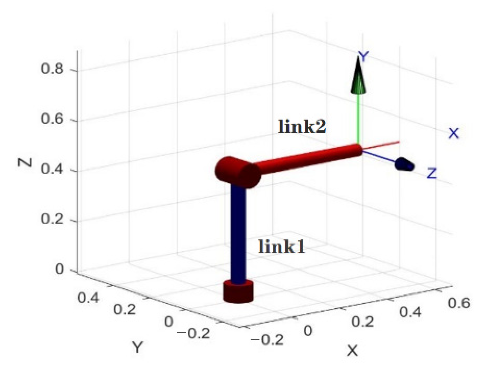
2. Materials and Methods

In this paper, the controlled object was selected as the n-joint manipulator, and its dynamic equation was:

$$M\left(q\right)\ddot{q}+C\left(q,\dot{q}\right)\dot{q}+G\left(q\right)=\tau -{\tau }_{\mathrm{d}}$$

(1)

where $M\left(q\right)$ is the$n\times n$ positive definite inertia matrix of the order; $C\left(q,\dot{q}\right)$ is for the$n\times n$ order centrifugation and Gohrenheit force terms; $G\left(q\right)$ is an$n\times 1$ order gravity term; the $q$ vectors are the joint variables; $\tau$ is the moment acting on the joint; and ${\tau }_{\mathrm{d}}$ is the disturbance for the outside world. In practical engineering, $M\left(q\right), C\left(q,\dot{q}\right)$, and$G\left(q\right)$ are often unknown factors and can be expressed as follows:

$$\begin{array}{ll}& M\left(q\right)=M_0\left(q\right)+E_{\mathrm{M}}\\ & C\left(q,\dot{q}\right)=C_0\left(q,\dot{q}\right)+E_{\mathrm{C}}\\ & G\left(q\right)=G_0\left(q\right)+E_{\mathrm{G}}\end{array}$$

(2)

where $E_{\mathrm{M}}, E_{\mathrm{C}}$, and $E_{\mathrm{G}}$ are modeled errors for$M\left(q\right), C\left(q,\dot{q}\right)$, and $G\left(q\right)$, respectively. The controller design defines the tracking error as:

$$e\left(t\right)=q_{\mathrm{d}}\left(t\right)-q\left(t\right)$$

(3)

where $q_{\mathrm{d}}\left(t\right)$ is the ideal tracking instructions and $q\left(t\right)$ is the actual location. The sliding mode function is defined as:

$$r=\dot{e}+\Lambda e$$

(4)

where $\Lambda >0$. ${\dot{q}}_{\mathrm{r}}=r\left(t\right)+\dot{q}\left(t\right)$ is defined, followed by${\ddot{q}}_{\mathrm{r}}=\dot{r}\left(t\right)+\ddot{q}\left(t\right), {\dot{q}}_{\mathrm{r}}={\dot{q}}_{\mathrm{d}}+\Lambda e$ and${\ddot{ q}}_{\mathrm{r}}={\ddot{q}}_{\mathrm{d}}+\Lambda {\dot{e}}^{\circ }$ by Equation (1), as follows:

$$\begin{array}{ll}\tau & =M\left(q\right)\ddot{q}+C\left(q,\dot{q}\right)\dot{q}+G\left(q\right)+{\tau }_{\mathrm{d}}\\ & =M\left(q\right)\left({\ddot{q}}_{\mathrm{r}}-\dot{r}\right)+C\left(q,\dot{q}\right)\left({\dot{q}}_{\mathrm{r}}-r\right)+G\left(q\right)+{\tau }_{\mathrm{d}}\\ & =M\left(q\right){\ddot{q}}_{\mathrm{r}}+C\left(q,\dot{q}\right){\dot{q}}_{\mathrm{r}}+G\left(q\right)-M\left(q\right)\dot{r}-C\left(q,\dot{q}\right)r+{\tau }_{\mathrm{d}}\\ & =M_0\left(q\right){\ddot{q}}_{\mathrm{r}}+C_0\left(q,\dot{q}\right){\dot{q}}_{\mathrm{r}}+G_0\left(q\right)+E^{\prime }-M\left(q\right)\dot{r}-C\left(q,\dot{q}\right)r+{\tau }_{\mathrm{d}}\end{array}$$

(5)

Among these $E^{\prime }=E_{\mathrm{M}}{\ddot{q}}_{\mathrm{r}}+E_{\mathrm{C}}{\dot{q}}_{\mathrm{r}}+E_{\mathrm{G} }$for the above system and the design controller is as follows:

$$\tau ={\tau }_{\mathrm{m}}+K_{\mathrm{p}}r+K_{\mathrm{i}}\int r\mathrm{d}t+{\tau }_{\mathrm{r}}$$

(6)

where $K_{\mathrm{p}}>0;K_{\mathrm{i}}>0;{\tau }_{\mathrm{m}}$ for the control term based on the nominal model; ${\tau }_{\mathrm{r}}$ is for robust terms and

$$\begin{array}{ll}& {\tau }_{\mathrm{m}}=M_0\left(q\right){\ddot{q}}_{\mathrm{r}}+C_0\left(q,\dot{q}\right){\dot{q}}_{\mathrm{r}}+G_0\left(q\right)\\ & {\tau }_r=K_{\mathrm{r}}\mathrm{sgn}\left(r\right)\end{array}$$

(7)

where $K_{\mathrm{r}}=\mathrm{diag}\left[k_{\mathrm{rii}}\right];k_{\mathrm{rii}}⩾\left|E_i\right|,i=1,\cdots ,n;E=E^{\prime }+{\tau }_{\mathrm{d}}$ is the coefficient matrix of the linear compensator. The purpose of this project was to design a controller through the Elman and RBF adaptive neural networks. Through simulation and training, the unknown external disturbance can be compensated more quickly, so as to obtain higher stability and shorten the system response time.

By synthesizing Equations (5)–(7), we can obtain:

$$\begin{array}{l}{M}_0\left(q\right){\ddot{q}}_{\mathrm{r}}+C_0\left(q,\dot{q}\right){\dot{q}}_{\mathrm{r}}+G_0\left(q\right)-M\left(q\right)\dot{r}-C\left(q,\dot{q}\right)r+E\prime +{\tau }_{\mathrm{r}}\\ =M_0\left(q\right){\ddot{q}}_{\mathrm{r}}+C_0\left(q,\dot{q}\right){\dot{q}}_{\mathrm{r}}+G_0\left(q\right)+K_{\mathrm{p}}r+K_{\mathrm{i}}{\int }_0^{t}r\mathrm{d}t+K_{\mathrm{r}}\mathrm{sgn}\left(r\right)\end{array}$$

(8)

where

$$M\left(q\right)\dot{r}+C\left(q,\dot{q}\right)r+K_{\mathrm{i}}{\int }_0^{t}r\mathrm{d}t=-K_{\mathrm{p}}r-K_{\mathrm{r}}\mathrm{sgn}\left(r\right)+E$$

(9)

Under this model, the traditional controller can only work under the unknown model and uncertainty, which causes the control input to chatter. To solve this problem, two kinds of neural networks were used to approximate the model and compensate for external disturbances.

3. Training of Nonlinear Neural Network Compensators

3.1. Designing Compensators with Elman Neural Networks

This part of the article is for the development of a model of an Elman neural control scheme for nonlinear dynamic systems in a manipulative robot.

As an example, consider an industrial n-link robot manipulator, the links of which are interconnected by rotational motion drives. The position of the links is determined by the angles ϕ₁, ϕ₂, ϕ₂… In addition, weight forces act on the robot links, which are directed at a certain angle α to the selected coordinate system, which demonstrates the ability of the device to work at any angle to the horizon [16].

The object of the control is the$n$ joint robotic arm, whose kinetic equation is:

$$M\left(q\right)\ddot{q}+C\left(q,\dot{q}\right)\dot{q}+G\left(q\right)+F\left(\dot{q}\right)+{\tau }_{\mathrm{d}}=\tau$$

(10)

Through the dynamic analysis of the manipulator in the second part and Equations (1)–(4), the following equations can be obtained:

$$\begin{array}{ll}M\dot{r}& =M\left({\ddot{q}}_{\mathrm{d}}-\ddot{q}+\Lambda \dot{e}\right)=M\left({\ddot{q}}_{\mathrm{d}}+\dot{e}\right)-M\ddot{q}\\ & =M\left({\ddot{q}}_{\mathrm{d}}+\Lambda \dot{e}\right)+C\dot{q}+G+F+{\tau }_{\mathrm{d}}-\tau \\ & =M\left({\ddot{q}}_{\mathrm{d}}+\Lambda \dot{e}\right)-Cr+C\left({\dot{q}}_{\mathrm{d}}+\Lambda e\right)+G+F+{\tau }_{\mathrm{d}}-\tau \\ & =-Cr-\tau +f+{\tau }_{\mathrm{d}}\end{array}$$

(11)

where $f\left(x\right)=M{\ddot{q}}_{\mathrm{r}}+C_{\mathrm{r}}+G+F;{\dot{q}}_{\mathrm{r}}={\dot{q}}_{\mathrm{d}}+\Lambda e$. As$f\left(x\right)$, you can see from the expression $f\left(x\right)$ that it contains all the model information—that is, in Equation (7), all the model information can be represented by$f\left(x\right)$. The control goal was to use the neural network approximation$f\left(x\right)$ to design a robust controller that does not require model information. The approximation used was Elman network approximation$f\left(x\right)$ and the network algorithm was:

$$\begin{array}{ll}& h_j=x_j\left(k-1\right), j=1,2,\cdots ,m\\ & f\left(x\right)=W{1}^{\top }h\left(k\right)+\mathrm{W}2\left(\mathrm{u}\left(k-1\right)\right)+\epsilon \end{array}$$

(12)

where $x$ is the input of the Elman neural network; $W$ is the ideal weights for the network;

W1 connect the weights from the input layer to the middle layer; W2 connects the weights from the output layer to the middle layer $h={\left[\begin{array}{llll}{h}_1\hfill & h_2\hfill & \cdots \hfill & h_m\hfill \end{array}\right]}^{\mathrm{T}}; \epsilon$ is a very small, positive real number. Approximation was carried out using Elman neural networks$f\left(x\right)$; j is the number of neurons in the hidden layer of the neural network.

The advantage of the Elman neural network is increased stability, since it has feedbacks from the outputs of internal neurons to the intermediate layer, which makes it more stable compared to a recurrent network of a similar type (for example, the Hopfield neural network, in which internal feedbacks are brought to the primary inputs, where signals are mixed). In addition, the Elman neural network allows you to take into account the background of the observed processes and accumulate information to choose the right robot control strategy [11].

$$\hat{f}\left(x\right)=\hat{W}{1}^{\top }h\left(k\right)+\hat{W}2\left(\mathrm{u}\left(k-1\right)\right)$$

where $\tilde{W}=W-\hat{W};\parallel W{\parallel }_F⩽W_{\max }$. Combining the above equation and Formula (12), we can get:

$$\begin{gathered} f-\hat{f}=W{1}^{\top }h\left(k-1\right)+\mathrm{W}2\left(k\right)+\epsilon -\hat{W}{1}^{\top }h\left(k\right)+\hat{W}2\left(\mathrm{u}(k-1\right)) \\ =\tilde{W}{1}^{\top }h\left(k-1\right)+\tilde{W}2\left(k\right)+\epsilon \end{gathered}$$

(13)

By Equation (13), referencing the$\left[11\right]$ design methods, the design control laws are:

$$\tau =\hat{f}\left(x\right)+K_{\mathrm{v}}r-v$$

(14)

where $v=-\left({\epsilon }_{\mathrm{N}}+b_{\mathrm{d}}\right)\mathrm{sgn}\left(r\right)$ for the robust term; $\hat{f}\left(x\right)$ is an approximation of $f\left(x\right)$. $\mathrm{ELMAN}$ The network weight adaptive law is:

$$\dot{\hat{W}}=\Gamma h{r}^{\mathrm{T}}$$

(15)

where $\Gamma ={\Gamma }^{\mathrm{T}}>0$. The general Equation (13) can be substituted into (10), a collation of the Elman neural network adaptive control MATLAB simulation:

$$\begin{array}{ll}M\dot{r}& =-Cr-\left(\hat{f}\left(x\right)+K_{\mathrm{v}}r-v\right)+f+{\tau }_{\mathrm{d}}\\ & =-\left(K_{\mathrm{v}}+C\right)r+\tilde{W}{1}^{\top }h\left(k\right)+\tilde{W}2\left(\mathrm{u}(k-1\right))+\epsilon +\left(\epsilon +{\tau }_{\mathrm{d}}\right)+v\\ & =-\left(K_{\mathrm{v}}+C\right)r+{\zeta }_{\mathrm{l}}\end{array}$$

(16)

where${\zeta }_1=\tilde{W}{1}^{\mathrm{T}}\left(k\right)\phi +W2\left(\mathrm{u}\left(\tilde{k}-1\right)\right)+\left(\epsilon +{\tau }_{\mathrm{d}}\right)+v_{ }$; with reference by [7], the analysis of the closed-loop system is as follows: the Lyapunov function is defined as:

$$L=\frac{1}{2}{r}^{\mathrm{T}}Mr+\frac{1}{2}\mathrm{tr}\left(\tilde{W}1{\left(k-1\right)}^{\mathrm{T}}{\Gamma }^{-1}\widetilde{W1\left(k\right)}\right)+\frac{1}{2}\mathrm{tr} \mathrm{u}\left(W2\left(\tilde{k}-1\right)\right)$$

(17)

Derivating Equation (17) to get:

$$\dot{L}=r^{\mathrm{T}}M\dot{r}+\frac{1}{2}{r}^{\mathrm{T}}\dot{M}r+\mathrm{tr}\left(\widetilde{\dot{\hat{W}}1{\left(k\right)}^{\mathrm{T}}}{\Gamma }^{-1}\dot{\overline{W1}}\right)+\mathrm{tru}\left(\widetilde{\dot{\hat{W}}2{\left(k-1\right)}^{\mathrm{T}}}{\Gamma }^{-1}\dot{\overline{W2}}\right)$$

By substituting Equation (15) into the above equation, the following Equation can be defined:

$$\begin{array}{ll}\dot{L}=& -r^{\mathrm{T}}{K}_{\mathrm{v}}r+\frac{1}{2}{r}^{\mathrm{T}}\left(\dot{M}-2C\right)r\\ & +\mathrm{tr}{\widetilde{W1\left(k\right)}}^{\mathrm{T}}\left({\Gamma }^{-1}\dot{W1}+h{r}^{\mathrm{T}}\right)+\mathrm{trW}2\left(k-1\right)\left({\Gamma }^{-1}\dot{W}2\right)+r^{\mathrm{T}}\left(\epsilon +{\tau }_{\mathrm{d}}+v\right)\end{array}$$

(18)

According to the following conditions:

(1)

oblique symmetry characteristics of the manipulator$r^{\mathrm{T}}\left(\dot{M}-2C\right)r=0$;

(2)

$r^{\mathrm{T}}{\tilde{W}}^{\mathrm{T}}h=\mathrm{tr}\left(W^{\mathrm{T}}h{r}^{\mathrm{T}}\right)$;

(3)

$\dot{\overrightarrow{W}}=-\dot{\hat{W}}=-\Gamma h{r}^{\mathrm{T}}$.

where

$$\dot{L}=-r^{\mathrm{T}}{K}_{\mathrm{v}}r+r^{\mathrm{T}}\left(\epsilon +{\tau }_{\mathrm{d}}+v\right)$$

(19)

consider

$$\begin{array}{ll}{r}^{\mathrm{T}}\left(\epsilon +{\tau }_{\mathrm{d}}+v\right)& =r^{\mathrm{T}}\left(\epsilon +{\tau }_{\mathrm{d}}\right)+r^{\mathrm{T}}\left(-\left({\epsilon }_{\mathrm{N}}+b_{\mathrm{d}}\right)\mathrm{sgn}\left(r\right)\right)\\ & =r^{\mathrm{T}}\left(\epsilon +{\tau }_{\mathrm{d}}\right)-\parallel r\parallel \left({\epsilon }_{\mathrm{N}}+b_{\mathrm{d}}\right)⩽0\end{array}$$

(20)

then the following definition can be obtained

$$\dot{L}⩽-r^{\mathrm{T}}{K}_{\mathrm{v}}r⩽0$$

(21)

The neural network learning algorithm consists of the following steps:

• At the initial moment of time t = 0, all neurons of the hidden layer are set to the zero position—the initial value is zero.
• The input value is fed to the network, where it is directly distributed.
• Set t = t + 1 and make the transition to step 2; neural network training is performed until the total root mean-square error of the network takes the smallest value.

3.2. Designing a Compensator with an Adaptive Radial Basis Function Neural Network for Local Model Approximation

In this section, a nonlinear dynamic model compensator is designed based on an Adaptive Radial basis function (RBF) neural network, based on the literature [8,11], which is then compared with the neural network compensator designed in the previous section.

The dynamic equation of the manipulator has the following properties:

Property 1: The inertia matrix$M_x\left(q\right)$ is symmetric positive definite;

Property 2: If $C_x\left(q,\dot{q}\right)$ is defined by Christoffel’s notation rule, the matrix ${\dot{M}}_x\left(q\right)-2C_x\left(q,\dot{q}\right)$ is skew symmetric [17].

Since $M_x\left(q\right)$ and $G_x\left(q\right)$ are just functions of $q$, they can be modeled using static neural networks [16,18,19,20].

$$\begin{array}{l}{m}_{xkj}\left(q\right)={\displaystyle \sum _l}{\theta }_{kij}{\xi }_{kij}\left(q\right)+{\epsilon }_{mkj}\left(q\right)={\theta }_{kj}^{\mathrm{T}}{\xi }_{kj}\left(q\right)+{\epsilon }_{mkj}\left(q\right)\\ g_{xk}\left(q\right)={\displaystyle \sum _l}{\beta }_{kl}{\eta }_{kl}\left(q\right)+{\epsilon }_{kk}\left(q\right)={\beta }_k^{\mathrm{T}}{\eta }_k\left(q\right)+{\epsilon }_{kk}\left(q\right)\end{array}$$

(22)

Among these, ${\theta }_{kjl},{\beta }_{kl}\in R$ are the weights of the neural network; ${\xi }_{kjl}\left(q\right),{\eta }_{kl}\left(q\right)\in R$ is the radial basis function whose input is a vector; $q$, ${\epsilon }_{mkj}\left(q\right),{\epsilon }_{kk}\left(q\right)\in R$ are the modeling errors of $m_{xkj}\left(q\right)$ and $g_{xk}\left(q\right)$, respectively, and are assumed to be bounded.

For $C\left(q,\dot{q}\right)$, modeling with a dynamic neural network with inputs $q$ and $q$, the neural network model of $C_{xkj}\left(q,\dot{q}\right)$ is:

$$C_{xkj}\left(q,\dot{q}\right)=\sum _l{\alpha }_{kil}{\xi }_{kil}\left(z\right)+{\epsilon }_{ikj}\left(z\right)={\alpha }_{kj}^{\mathrm{T}}{\xi }_{kj}\left(z\right)+{\epsilon }_{ikj}\left(z\right)$$

(23)

Among these, $z={\left[\begin{array}{ll}{q}^{\mathrm{T}}\hfill & {\dot{q}}^{\mathrm{T}}\hfill \end{array}\right]}^{\mathrm{T}}\in R^{2n};{\alpha }_{kjl}\in R$ is the weight; ${\xi }_{kjl}\left(z\right)\in R$ is the radial basis function of the input vector $z$; and ${\epsilon }_{ckj}\left(z\right)$ is the modeling error of the element $c_{xkj}\left(q,\dot{q}\right)$, assuming it is also bounded [20,21].

Using neural network modeling, the dynamic equation of the manipulator in space can be written as:

$$M_x\left(q\right)\ddot{x}+C_x\left(q,\dot{q}\right)\dot{x}+G_x\left(q\right)=F_x$$

(24)

Using GL (general linear) matrices and their multiplication operations, $M_x\left(q\right)$ can be written as:

$$M_x\left(q\right)=\left[{\{\theta \}}^{\top }·\left\{\Xi \left(q\right)\right\}\right]+E_{\mathrm{M}}\left(q\right)$$

(25)

where {θ} and {Ξ(q)} are GL (general linear) matrices whose elements are ${\theta }_{kj}^{\mathrm{T}}$ and ${\xi }_{kj}\left(q\right)$; E_M (q)∈R^(n × n) is a matrix whose elements are modeling errors ${\epsilon }_{mkj}\left(q\right)$.

Similarly, for $C\left(q,\dot{q}\right)$ and $G_x\left(q\right)$:

$$C_x\left(q,q \dot{}\right)=\left[{\left\{A\right\}}^T·\left\{Z\left(z\right)\right\}\right]+E_C\left(z\right) G\_x \left(q\right)=\left[\left\{B\right\}^T·\left\{H\left(q\right)\right\}\right]+E\_G \left(q\right))$$

(26)

where $\left\{A\right\},\left\{Z\left(z\right)\right\}, \left\{B\right\}$, and $\left\{H\left(q\right)\right\}$ are GL matrices and GL vectors whose elements are ${\alpha }_{kj}, {\xi }_{kj}\left(z\right), {\beta }_k$ and ${\eta }_k\left(q\right);E_{\mathrm{C}}\left(z\right)\in R^{n\times n}$ and $E_{\mathrm{G}}\left(q\right)\in R^n$ are the elements and matrices of the modeling errors ${\epsilon }_{\mathrm{c}kj}\left(z\right)$ and ${\epsilon }_{kk}\left(q\right)$, respectively.

Assuming $x_d\left(t\right)$ is the ideal trajectory of the workspace, then$\dot{ x_d}\left(t\right)$ and $\ddot{x_d}\left(t\right)$ are the ideal velocity and ideal acceleration:

$$\begin{array}{ll}& {\dot{x}}_{\mathrm{r}}\left(t\right)={\dot{x}}_{\mathrm{d}}\left(t\right)+\Lambda e\left(t\right)\\ & r\left(t\right)={\dot{x}}_{\mathrm{r}}\left(t\right)-\dot{x}\left(t\right)=\dot{e}\left(t\right)+\Lambda e\left(t\right)\end{array}$$

(27)

where $\Lambda$is a positive definite matrix.

Lemma 1 (Barbalat’s Lemma).

If the function $h:R\to R$ is a uniform continuous function defined by $[0,+\infty$ ), and ${\lim }_{t\to \infty }{\int }_0^{t}h\left(\delta \right)\mathrm{d}$ exists and is finite, then ${\lim }_{t\to \infty }h\left(t\right)=0$ is obtained [22].

Lemma 2.

Let $e\left(t\right)=h\left(t\right)*r\left(t\right)$, where * represents convolution, $h\left(t\right)=L^{-1}H\left(s\right)$andH(s) is a strictly exponentially stable transfer function of order n * n. If $r\in L_2^n$, then$e\in L_2^n\cap L_{\infty }^n,\dot{e}\in L_2^n,e$ is continuous, $e\to 0,r\to 0,\dot{e}\to 0$ when $t\to \infty$.

Consider a second-order SISO system and let $r\left(t\right)=ce\left(t\right)+\dot{e}\left(t\right)$, then we can obtain $r\left(s\right)=e\left(s\right)\left(c+s\right)$, $e\left(s\right)=$ $\frac{1}{s+c}r\left(s\right)$, and $H\left(s\right)=\frac{1}{s+c}$. To ensure that H(s) is a strictly exponentially stable transfer function, it can be defined that c > 0. If the above conditions are satisfied, then $r\left(t\right)=0$, ce(t) + e(t) = 0 can be obtained, thus ensuring that the system is exponentially closed [17].

Using $\left(\hat{\sigma }\right)$ to represent the estimated value of $\left(·\right)$, define $d\left(·\right)=\left(·\right)-\left(\hat{\sigma }\right)$, then $\left\{\hat{\theta }\right\},\left\{\hat{A}\right\}$, and $\left\{\hat{B}\right\}$ represents the $\left\{\theta \right\},\left\{A\right\}$, and $\left\{B\right\}$ estimates.

Designing the controller this can be defined as:

$$F_x=\left[{\left\{\hat{\theta }\right\}}^{\mathrm{T}}·\left\{\theta \left(q\right)\right\}\right]{\ddot{x}}_{\mathrm{r}}+\left[{\left\{\hat{A}\right\}}^{\mathrm{T}}·\left\{Z\left(z\right)\right\}\right]{\dot{x}}_{\mathrm{r}}+\left[{\left\{\hat{B}\right\}}^{\mathrm{T}}·\left\{H\left(q\right)\right\}\right]+Kr+k_{\mathrm{s}}\mathrm{sgn}\left(r\right)$$

(28)

where $K\in R^{n\times n}>0;k_{\mathrm{s}}>\parallel E\parallel ;E=E_{\mathrm{M}}\left(q\right){\ddot{x}}_{\mathrm{r}}+E_{\mathrm{C}}\left(z\right){\dot{x}}_{\mathrm{r}}+E_{\mathrm{G}}\left(q\right)$. The first three terms of the controller are model-based controls, the K_r term is equivalent to the proportional derivative (PD) control, and the last term of the control law is a robust term that suppresses the modeling error of the neural network.

From the expression of the controller, it is obvious that the controller does not need to solve the Jacobian inverse matrix. In actual control, the loser can be obtained by $\tau =J^{\mathrm{T}}\left(q\right)F_x \left[19\right]$.

Substituting Equations (24) and (25) into Equation (23), we can obtain:

$$\begin{array}{ll}& \left\{\left[{\{\theta \}}^{\mathrm{T}}·\left\{\Xi \left(q\right)\right\}\right]+E_{\mathrm{M}}\left(q\right)\right\}\ddot{x}+\left\{\left[{\left\{A\right\}}^{\mathrm{T}}·\left\{Z\left(z\right)\right\}\right]+E_{\mathrm{C}}\left(z\right)\right\}\dot{x}\\ & +\left[{\left\{B\right\}}^{\mathrm{T}}·\left\{H\left(q\right)\right\}\right]+E_{\mathrm{G}}\left(q\right)=F_x\end{array}$$

(29)

Substituting the control law (27) into the above formula, we can obtain:

$$\begin{array}{ll}& \left\{\left[{\{\theta \}}^{\mathrm{T}}·\left\{E\left(q\right)\right\}\right]+E_{\mathrm{M}}\left(q\right)\right\}\ddot{x}+\left\{\left[{\left\{A\right\}}^{\mathrm{T}}·\left\{Z\left(z\right)\right\}\right]\right.\\ & \left.+E_{\mathrm{C}}\left(z\right)\right\}\dot{x}+\left[{\left\{B\right\}}^{\mathrm{T}}·\left\{H\left(q\right)\right\}\right]+E_{\mathrm{G}}\left(q\right)\\ =& \left[{\left\{\hat{\theta }\right\}}^{\mathrm{T}}·\left\{\Xi \left(q\right)\right\}\right]{\ddot{x}}_{\mathrm{r}}+\left[{\left\{\hat{A}\right\}}^{\mathrm{T}}·\left\{Z\left(z\right)\right\}\right]{\dot{x}}_{\mathrm{r}}\\ & +\left[{\left\{\hat{B}\right\}}^{\mathrm{T}}·\left\{H\left(q\right)\right\}\right]+Kr+k_{\mathrm{s}}\mathrm{sgn}\left(r\right)\end{array}$$

(30)

Substituting X =${\dot{ x}}_{\mathrm{r}}-r$ and ${\ddot{x}}_{\mathrm{r}}$=${\ddot{ x}}_{\mathrm{r}}-\dot{r}$ into the above equation, we can obtain:

$$\begin{array}{ll}& \left\{\left[{\{\theta \}}^{\mathrm{T}}·\left\{\theta \left(q\right)\right\}\right]+E_{\mathrm{M}}\left(q\right)\right\}\left({\ddot{x}}_{\mathrm{r}}-\dot{r}\right)+\left\{\left[{\left\{A\right\}}^{\mathrm{T}}·\left\{Z\left(z\right)\right\}\right]\right.\\ & \left.+E_{\mathrm{C}}\left(z\right)\right\}\left({\dot{x}}_{\mathrm{r}}-r\right)+\left[{\left\{B\right\}}^{\mathrm{T}}·\left\{H\left(q\right)\right\}\right]+E_{\mathrm{G}}\left(q\right)\\ =& \left[{\left\{\hat{\theta }\right\}}^{\mathrm{T}}·\left\{\theta \left(q\right)\right\}\right]{\ddot{x}}_{\mathrm{r}}+\left[{\left\{\hat{A}\right\}}^{\mathrm{T}}·\left\{Z\left(z\right)\right\}\right]{\dot{x}}_{\mathrm{r}}+\left[{\langle \hat{B}\rangle }^{\top }·\{H\left(q\right)\rangle \right]+Kr+k_s\mathrm{sgn}\left(r\right)\end{array}$$

(31)

Substituting Equations (24) and (25) into the above equations, we can obtain:

$$\begin{array}{ll}& M_f\left(q\right)\dot{r}+C_x\left(q,\dot{q}\right)r+Kr+k_s\mathrm{sgn}\left(r\right)\\ =& \left[{\left\{\theta \right\}}^{\top }·\langle B\left(q\right)\}\right]{\ddot{x}}_{\mathrm{r}}+\left[\{\hat{A}{\rangle }^{\top }·\left\{Z\left(z\right)\right\}\right]{\dot{x}}_{\mathrm{r}}+\left[{\{\tilde{B}\}}^{\top }·\left\{H\left(q\right)\right\}\right]+E\end{array}$$

(32)

For the closed-loop system, if $K>0,k,>\parallel E\parallel$ parallel, and the adaptive law is designed as:

$$\begin{array}{ll}{\dot{\hat{\theta }}}_k& ={\Gamma }_k·\left\{{\xi }_k\left(q\right)\right\}{\ddot{x}}_t{r}_k\\ {\dot{\hat{\alpha }}}_k& =Q_k·\left\{{\xi }_k\left(z\right)\right\}{\dot{x}}_r{r}_k\\ {\dot{\hat{\beta }}}_k& =N_{\downarrow }{\eta }_k\left(q\right)r_k\end{array}$$

(33)

Among these, ${\Gamma }_k={\Gamma }_k^T>0;Q_k=Q_k^T>0;N_k=N_k^T>0$ and ${\hat{\theta }}_k$ and ${\hat{\alpha }}_k$ are the vectors of ${\hat{\theta }}_k$ and ${\hat{a}}_k$, respectively; then, ${\hat{\theta }}_k$, ${\hat{\alpha }}_t·{\hat{\beta }}_k\in L\dots ,e\in L_2^{*}\cap L^{*},e$ is continuous. And $e\to 0$ and $\dot{e}\to 0$ when $t\to \infty$.

According to an integral line Lyapunov function proposed in Reference, the stability can be analyzed as follows:

$$RV=\frac{1}{2}{r}^{\mathrm{T}}{M}_k\left(q\right)r+\frac{1}{2}\sum _{k=1}^n{\theta }_k^{\mathrm{T}}{\Gamma }_k^{-1}{\theta }_k+\frac{1}{2}\sum _{k=1}^n{\stackrel{\sim }{\alpha }}_k^{\mathrm{T}}{Q}_k^{-1}{\stackrel{\sim }{\alpha }}_k+\frac{1}{2}\sum _{k=1}^n{\hat{\beta }}_k^{\mathrm{T}}{N}_k^{-1}{\hat{\beta }}_k$$

(34)

Among these, ${\Gamma }_k, Q_k, \mathrm{and} N_{k }$are positive definite pair-second matrices. Derivative with respect to V, we obtain:

$$R\dot{V}=r^{\mathrm{T}}{M}_k\dot{r}+\frac{1}{2}{r}^{\mathrm{T}}{\dot{M}}_{k}r+\sum _{k=1}^n{\overline{\theta }}_k^{\mathrm{T}}{\Gamma }_k^{-1}{\dot{\theta }}_k+\sum _{k=1}^n{\alpha }_k^{\mathrm{T}}{Q}_k^{-1}{\dot{\alpha }}_k+\sum _{k=1}^n{\hat{\beta }}_k^{\mathrm{T}}{N}_k^{\prime }{\dot{\beta }}_k$$

(35)

Since the matrix ${\dot{M}}_x\left(q\right)-2C_x\left(q,\dot{q}\right)$ is obliquely symmetric, then $r^{\mathrm{T}}\left({\dot{M}}_x-2C_x\right)r=0$, and the below formula can be obtained:

$$\dot{V}=r^{\top }\left(M_s\dot{r}+C_{s}r\right)-\sum _{k=1}^n{\overline{\theta }}_k^{\top }{\Gamma }_k^{-1}{\stackrel{\dot{^}}{\theta }}_k+\sum _{k=1}^n{\alpha }_l^{\top }{Q}_k^{-1}{\dot{\alpha }}_k-\sum _{k=1}^n{\overline{\beta }}_k^{\top }{N}_k^{-1}{\stackrel{\dot{^}}{\beta }}_k$$

(36)

Substituting Equation (33) into the above equation, we can obtain:

$$\begin{array}{ll}\dot{V}=& -r^{\top }Kr-k_s{r}^{\top }\mathrm{sgn}\left(r\right)+{\displaystyle \sum _{k=1}^n}\langle {\theta }_k{\}}^{\top }·\{{\xi }_k\left(q\right)\}{\ddot{x}}_t{r}_k+{\displaystyle \sum _{k=1}^n}{\stackrel{\sim }{\alpha }}_k^{\top }·\langle {\xi }_k\left(z\right)\rangle {\dot{x}}_{*}{r}_k\\ & +{\displaystyle \sum _{k=1}^n}{\beta }_k^{\top }{\eta }_k\left(q\right)r_k+r^{\top }E-{\displaystyle \sum _{k=1}^n}{\theta }_k^{\top }{\Gamma }_k^{\prime }{\stackrel{\dot{^}}{\theta }}_k+{\displaystyle \sum _{k=1}^n}{\alpha }_k^{\top }{Q}_k^{-}{\stackrel{\dot{^}}{\alpha }}_k-{\displaystyle \sum _{k=1}^n}{\hat{\beta }}_k^{\top }{N}_k^{-1}{\stackrel{\dot{^}}{\beta }}_k\end{array}$$

(37)

Substituting the adaptive law (32) into the Equation (37), and combining the inequality $k_n>\parallel E\parallel$ parallel, we can obtain:

$$\dot{V}=-r^{\mathrm{T}}Kr-k_x{r}^{\mathrm{T}}\mathrm{sgn}\left(r\right)+r^{\mathrm{T}}E⩽0$$

(38)

Convergence Analysis:

(1)

From $\dot{V}⩽-r^{\top }Kr⩽0$ and $K>0$, from the lemma $e\in L_2^n\cap L^n,\dot{e}\in L_2^n,e$, e∈L2n, e is continuous; then, when $t\to \infty$, $e\to 0,\dot{e}\to 0$

(2)

From $\dot{V}⩽-r^{\top }K$, we get $0⩽V\left(t\right)⩽V\left(0\right),\forall t⩾0$. Therefore, when $V\left(t\right)\in L$, there are${\theta }_k$,${\hat{\alpha }}_k,{\beta }_k\in L, \mathrm{and} {\hat{\theta }}_k,{\hat{\alpha }}_k,{\hat{\beta }}_k\in L$.

4. Simulation Study

This section presents the simulation results to evaluate the operation of the proposed adaptive neuro controller. In this section, the proposed control scheme is applied to a two-link project, the mathematical model of which was developed in the Solid works package and imported in the MATLAB package by the second generation of Simulink [22,23].

Initially, the first link moves, but the second one does not. It is shown that after the training of the first link, external disturbances are worked out. Then, the second link starts moving, and the first one stops. After that, both links move, exerting dynamic disturbances on each link. The dynamic equation can be written as:

$$M\left(q\right)\ddot{q}+C\left(q,\dot{q}\right)\dot{q}+G\left(q\right)=\tau -d$$

$$M\left(q\right)=\left[\begin{array}{cc}q1+2\gamma \cos \left(q2\right)& q1+q2\cos \left(q2\right)\\ q1+q2\cos \left(q2\right)& q1\end{array}\right]$$

$$C\left(q,\dot{q}\right)=\left[\begin{array}{cc}-q2\dot{ q}2\sin \left(q2\right)& -q2\left(\dot{q}1+\dot{ q}2\right)\sin \left(q2\right)\\ q2 \dot{q1\sin \left(q2\right)}& 0\end{array}\right]$$

$$G\left(q\right)=\left[\begin{array}{c}g\cos q1+g \cos \left(q1+q2\right)\\ g \cos \left(q1+q2\right)\end{array}\right]$$

where the known parameters are j = 12, q1 = 9, q2 = 8, g = 9.8 [23] and the external interferences of the system are $d=d1+d2e+d\dot{e}$, d1 = 2, d2 = 3, d3 = 6. Assuming that the expected instructions for tracking the link angle and angular velocity are the following equation:

$$q1d=1+0.2\sin \left(0.5\pi t\right)$$

$$q2d=1-0.2\cos \left(0.5\pi t\right)$$

then the initial state of the system is [q1 q2]^T = [0.6 0.3]^T, $\Delta M=0.6M$, $\Delta C=0.6C,\Delta G=0.6G$. When modeling, using the formula of the control law and the formula of the adaptive law, $\alpha =2, \gamma =20,k=0.001$. In the neural network, the parameters of the Gaussian function were set to c = [−2 −1 0 1 2] and b = 3, and the initial weight was 0.1. The model of the manipulator is shown in Figure 1.

The simulation parameters of the robotic arm were as follows:

L(1): ‘qlim’, [−180 180] * deg; ‘m’, 0,… ‘Jm’, 200 × 10⁻⁶,… ‘G’, −62.6111,… ‘B’, 1.48 × 10⁻³

L(2): ‘qlim’, [−180 180] * deg; ‘m’, 17.4,… ‘Jm’, 200 × 10⁻⁶,… ‘G’, 107.815,… ‘B’, 0.817 × 10⁻³

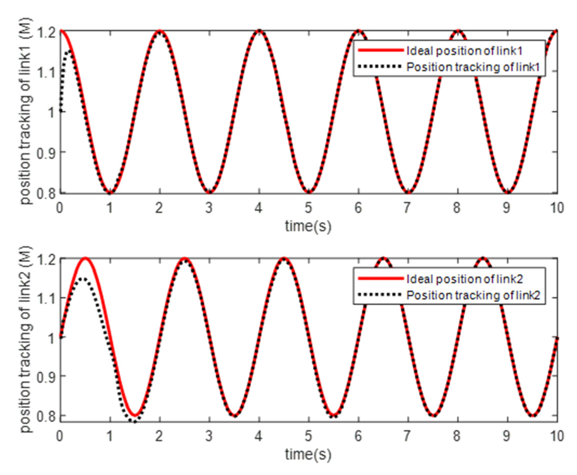
(1)

Simulation Modeling of Elman Neural Networks

In the Matlab/Simulink system, an artificial neural network model was created to control a manipulative robot, containing an input layer of 15 neurons and a hidden layer varying from 12 to 19 neurons that have local feedback through delay lines.

It can be seen from the Figure 2 and Figure 3 that in the case of adaptive compensation, there was a certain degree of disturbance at the initial stage, and the angular velocity and position tended to converge.

It can be seen from the Figure 4 that the disturbances were compensated and that the robot control process was quite satisfactory.

The experimental results also demonstrate that the proposed method was sufficiently resistant to dynamic perturbations due to unknown situations. The proposed control method is original and successfully exploits the advantages of SMC, neural networks, and adaptive control.

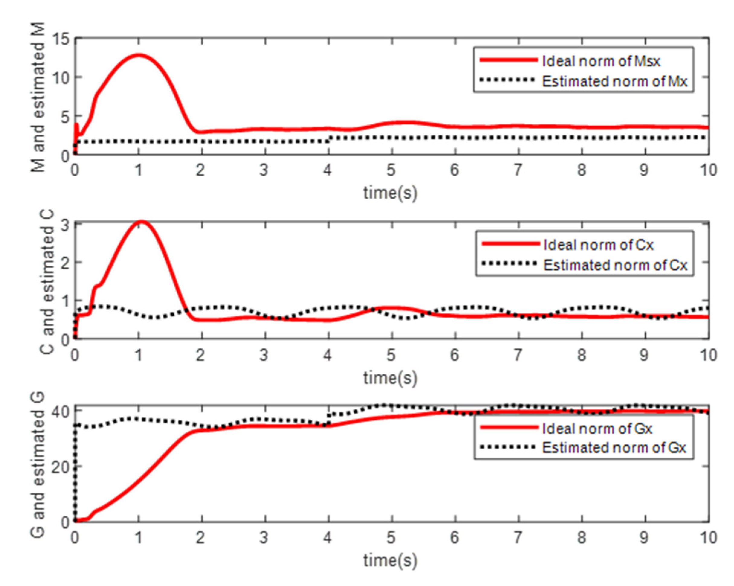
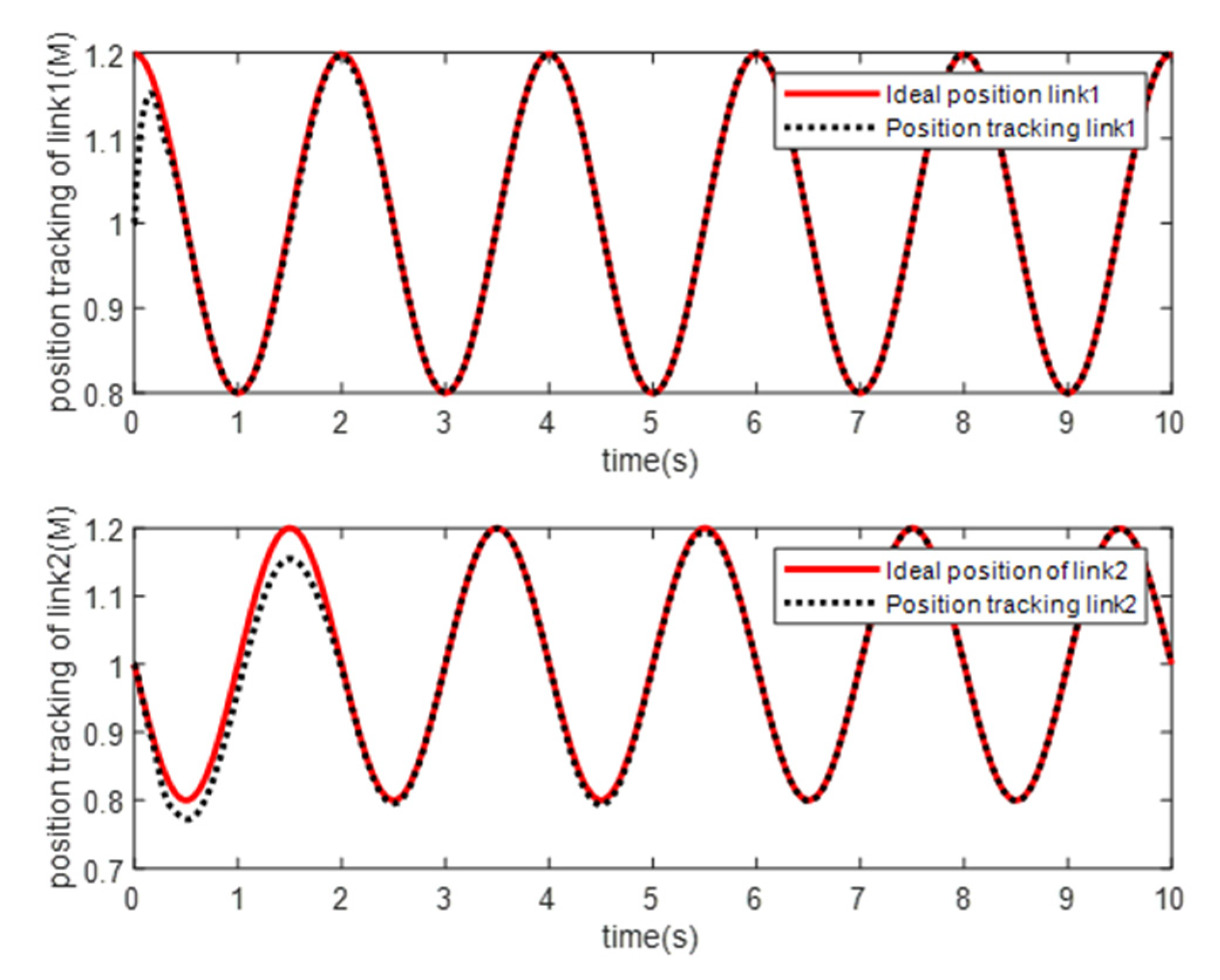
(2)

Simulation Modeling of RBF Neural Networks

For the approximation of each element of $M_x\left(q\right)$ and $G_x\left(q\right)$, it is assumed that the input vector of the RBF neural network is q and the number of hidden layer points is nine. For $C_x\left(q,\dot{q}\right)$, the input vector $\left(q,\dot{q}\right)$ of the RBF neural network is assumed and the number of design hidden layer points is seven.

The parameters of all Gaussian functions are taken as $c_i=\left[\begin{array}{lllllll}-1.5\hfill & -1.0\hfill & -0.5\hfill & 0\hfill & 0.5\hfill & 1.0\hfill & 1.5\hfill \end{array}\right]$ and $b_i=$ 10, The initial threshold of the neural network is set to zero in the simulation. The control law adopts Formula (26), and the adaptive law adopts Formula (31). The benefit is chosen as $K=\left[\begin{array}{cc}30& 0\\ 0& 30\end{array}\right],k_{\mathrm{s}}=0.5$. From Lemma 2, it is desirable that $\Lambda =\left[\begin{array}{cc}15& 0\\ 0& 15\end{array}\right]$. The parameters of the adaptive law (31) are taken as \${\Gamma }_k=\mathrm{diag}\left\{2.0\right\},Q_k=\mathrm{diag}\left\{0.10\right\}$ and $N_k=\mathrm{diag}\left\{5.0\right\}$. The simulation results are shown in Figure 5 and Figure 6.

As can be seen from the Figure 5 and Figure 6, at the beginning of the simulation, the error value was relatively large due to the neural network learning phase of the control input. When the neural network compensator passed the learning stage, the errors were basically eliminated, and the motion trajectory and the estimated value converged in the RBF neural network relatively quickly, but the neural network training and compensation accuracy were lower than Elman neural network. The unknown perturbation was almost completely cancelled after 1 s.

From Figure 7 can be seen that since the tracking trajectory was not a continuous excitation, the estimated values $\parallel {\hat{M}}_x\left(q\right)\parallel , \parallel {\hat{C}}_x\left(q,\dot{q}\right)\parallel ,$and $\parallel {\hat{G}}_x\left(q\right)\parallel$ did not converge to $\parallel M_x\left(q\right)\parallel , \parallel C_x\left(q,\dot{q}\right)\parallel$, and $\parallel G_x\left(q\right)\parallel$, which is often encountered in practical engineering.

From the simulation of the two neural networks, it can be seen from Figure 8 and Figure 9 that although the RBF neural network has faster training and learning speed under the same trajectory planning. But Elman neural network is better in terms of compensation accuracy for external disturbances and errors. However, when there were more interference conditions and uncertain environments, the overall training results of the RBF were better.

In theory, as enough neurons are added to the hidden layer of the Elman network, higher learning expectations will be obtained. However, in the actual simulation, once the number of neurons in the hidden layer exceeds 60, the neural network will be in a state of over-learning and the accuracy will drop.

5. Conclusions

Therefore, summarizing the research results, the following conclusions can be drawn: During the research process, the quality of a robot to perform a specific task depends not only on the quality of the manufacturing materials and the quality of the moving parts, but also on the quality of the mathematical model of the robot. The control efficiency and accuracy of the robot is based on the analysis of its dynamic model, reducing the error between the planned trajectory and the actual trajectory. This paper presents two different neural networks for manipulating nonlinear dynamic systems of robots by developing models of adaptive neural control schemes based on Elman networks. The choice of network architecture is sound. Simulations of the RBF adaptive neural network show that, despite the faster response time, in the absence of continuous excitation, the system does not converge and the error value is much larger than that of the Elman network. However, if the simulation is performed locally, or if the system dynamics structure is complex and there are many external disturbances, the response time and accuracy of the RBF adaptive neural network will be better. The rotation model of the planar manipulator is described by the dynamic model equation and the output equation. The simulation and training of an adaptive neural network controller confirms its use in the presence of imprecise dynamic structural data and unknown external disturbances. A computer simulation was applied to the optimal control model, tracking the rotation angle of the manipulator, which confirmed the theoretical position and demonstrated its high operating efficiency. This method can also be applied to the simulation of multi-degree-of-freedom manipulators. At the same time, the improved model can be used for the adaptive control method of the manipulator.

References

- Duka, A.V. Neural Network based Inverse Kinematics Solution for Trajectory Tracking of a Robotic Arm. Procedia Technol. 2014, 12, 20–27. [Google Scholar] [CrossRef]
- Arseniev, D.G.; Overmeyer, L.; Kälviäinen, H.; Katalinić, B. Cyber-Physical Systems and Control; Springer: Berlin/Heidelberg, Germany, 2019. [Google Scholar]
- Islam, S.; Liu, X.P. Robust Sliding Mode Control for Robot Manipulators. IEEE Trans. Ind. Electron. 2011, 58, 2444–2453. [Google Scholar] [CrossRef]
- Yazdanpanah, M.J.; KarimianKhosrowshahi, G. Robust Control of Mobile Robots Using the Computed Torque Plus H∞ Compensation Method. Available online: https://www.sciencegate.app/document/10.1109/cdc.2003.1273069 (accessed on 29 June 2022).
- Rostova, E.N.; Rostov, N.V.; Yan, Y.Z. Neural network compensation of dynamic errors in a position control system of a robot manipulator. Comput. Telecommun. Control. 2020, 64, 53–64. [Google Scholar] [CrossRef]
- Yesildirak, A.; Lewis, F.W.; Yesildirak, S.J. Neural Network Control of Robot Manipulators and Non-Linear Systems; CRC Press: Boca Raton, FL, USA, 2020. [Google Scholar]
- Kara, K.; Missoum, T.E.; Hemsas, K.E.; Hadjili, M.L. Control of a robotic manipulator using neural network based predictive control. 2010. In Proceedings of the 17th IEEE International Conference on Electronics, Circuits and Systems, Athens, Greece, 12–15 December 2010; pp. 1104–1107. [Google Scholar] [CrossRef]
- Seshagiri, S.; Khalil, H. Output Feedback Control of Nonlinear Systems Using RBF Neural Networks. IEEE Trans. Neural Netw. 2000, 11, 69–79. [Google Scholar] [CrossRef] [PubMed]
- Tetko, V.I.; Kůrková, V.; Karpov, P.; Theis, F. Artificial Neural Networks and Machine Learning–ICANN 2019: Deep Learning: 28th International Conference on Artificial Neural Networks, Munich, Germany, September 17–19, 2019, Proceedings, Part II; Springer: Berlin/Heidelberg, Germany, 2019. [Google Scholar]
- Dou, M.; Qin, C.; Li, G.; Wang, C. Research on Calculation Method of Free flow Discharge Based on Artificial Neural Network and Regression Analysis. Flow Meas. Instrum. 2020, 72, 101707. [Google Scholar] [CrossRef]
- Ren, G.; Cao, Y.; Wen, S.; Huang, T.; Zeng, Z. A Modified Elman Neural Network with a New Learning Rate Scheme. Neurocomputing 2018, 286, 11–18. [Google Scholar] [CrossRef]
- Design and Implementation of a RoBO-2L MATLAB Toolbox for a Motion Control of a Robotic Manipulator. Available online: https://ieeexplore.ieee.org/document/7473678/ (accessed on 30 June 2022).
- Cheng, Y.-C.; Qi, W.-M.; Cai, W.-Y. Dynamic properties of Elman and modified Elman neural network. In Proceedings of the International Conference on Machine Learning and Cybernetics, Beijing, China, 4–5 November 2002; pp. 637–640. [Google Scholar] [CrossRef]
- Beheim, L.; Zitouni, A.; Belloir, F. New RBF neural network classifier with optimized hidden neurons number. WSEAS Trans. Syst. 2004, 2, 467–472. [Google Scholar]
- Song, Q.; Meng, G.J.; Yang, L.; Du, D.Q.; Mao, X.F. Comparison between BP and RBF Neural Network Pattern Recognition Process Applied in the Droplet Analyzer. Appl. Mech. Mater. 2014, 543–547, 2333–2336. [Google Scholar] [CrossRef]
- Luo, B.; Liu, D.; Yang, X.; Ma, H. H ∞ Control Synthesis for Linear Parabolic PDE Systems with Model-Free Policy Iteration. In Advances in Neural Networks—ISNN 2015; Springer: Berlin/Heidelberg, Germany, 2015; pp. 81–90. [Google Scholar] [CrossRef]
- Ge, S.S.; Hang, C.C.; Woon, L.C. Adaptive neural network control of robot manipulators in task space. IEEE Trans. Ind. Electron. 1997, 44, 746–752. [Google Scholar] [CrossRef]
- Chen, C.; Liu, Z.; Xie, K.; Zhang, Y.; Chen, C.L.P. Adaptive neural control of MIMO stochastic systems with unknown high-frequency gains. Inf. Sci. 2017, 418, 513–530. [Google Scholar] [CrossRef]
- Chen, Y.; Liu, J.; Wang, H.; Pan, Z.; Han, S. Model-free based adaptive RBF neural network control for a rehabilitation exoskeleton. In Proceedings of the 2019 Chinese Control and Decision Conference (CCDC), Nanchang, China, 3–5 June 2019; pp. 4208–4213. [Google Scholar] [CrossRef]
- Wang, M.; Yang, A. Dynamic Learning from Adaptive Neural Control of Robot Manipulators with Prescribed Performance. IEEE Trans. Syst. Man Cybern. Syst. 2017, 47, 2244–2255. [Google Scholar] [CrossRef]
- Tran, M.-D.; Kang, H.-J. Nonsingular Terminal Sliding Mode Control of Uncertain Second-Order Nonlinear Systems. Math. Probl. Eng. 2015, 2015, e181737. [Google Scholar] [CrossRef]
- Ortega, R.; Spong, M.W. Adaptive motion control of rigid robots: A tutorial. In Proceedings of the 27th IEEE Conference on Decision and Control, Austin, TX, USA, 7–9 December 1988; pp. 1575–1584. [Google Scholar] [CrossRef]
- Zabikhifar, S.; Markasi, A.; Yuschenko, A. Two link manipulator control using fuzzy sliding mode approach. Her. Bauman Mosc. State Tech. Univ. Ser. Instrum. Eng. 2015, 6, 30–45. [Google Scholar] [CrossRef]
Publisher’s Note: MDPI stays neutral with regard to jurisdictional claims in published maps and institutional affiliations. |
© 2022 by the authors. Licensee MDPI, Basel, Switzerland. This article is an open access article distributed under the terms and conditions of the Creative Commons Attribution (CC BY) license (https://creativecommons.org/licenses/by/4.0/).
Share and Cite
Yan, Z.; Klochkov, Y.; Xi, L. Improving the Accuracy of a Robot by Using Neural Networks (Neural Compensators and Nonlinear Dynamics). Robotics 2022, 11, 83. https://doi.org/10.3390/robotics11040083
Yan Z, Klochkov Y, Xi L. Improving the Accuracy of a Robot by Using Neural Networks (Neural Compensators and Nonlinear Dynamics). Robotics. 2022; 11(4):83. https://doi.org/10.3390/robotics11040083
Chicago/Turabian StyleYan, Zhengjie, Yury Klochkov, and Lin Xi. 2022. "Improving the Accuracy of a Robot by Using Neural Networks (Neural Compensators and Nonlinear Dynamics)" Robotics 11, no. 4: 83. https://doi.org/10.3390/robotics11040083
APA StyleYan, Z., Klochkov, Y., & Xi, L. (2022). Improving the Accuracy of a Robot by Using Neural Networks (Neural Compensators and Nonlinear Dynamics). Robotics, 11(4), 83. https://doi.org/10.3390/robotics11040083