1. Introduction
Robotics systems were first introduced as a technical means for the automation of production processes. Hard labour has since then been reduced in terms of both basic and auxiliary technical operations. Practice demonstrated that auxiliary operations, which are monotonous and often strenuous, were hard to automate in the traditional sense [
1]. Hence, a deeper realisation and broad application of industrial robotics arose. The robotic systems that perform motion in a form similar to actual human arm movements are generally listed into the following three categories:
Industrial development has been primarily accomplished with the use of various types of robotic manipulation systems. For the movement and manipulation of these systems, kinematic modelling is utilised.
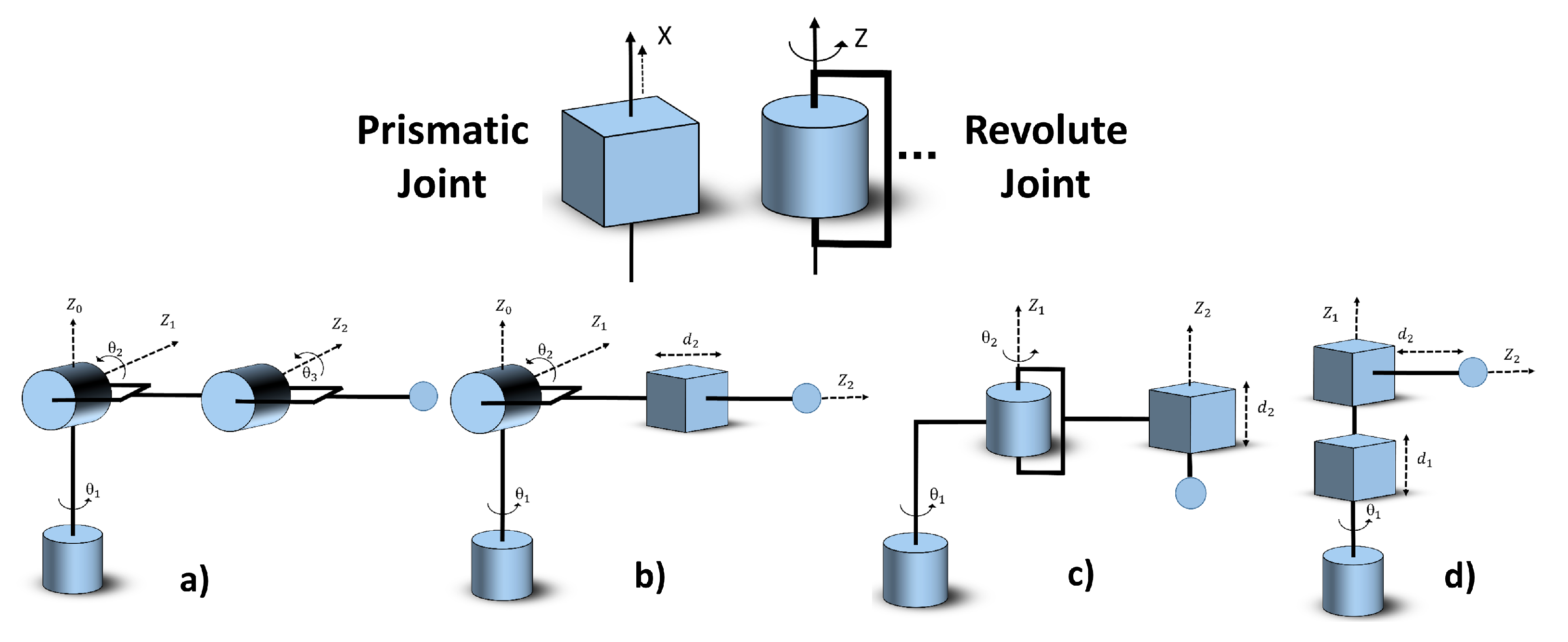
Kinematics is a category of classical mechanics which is responsible for the study of physical motion, minus the consideration of forces and momentum. Robotic kinematics provide the fundamental components for mathematical modelling and analysis for the structure of robotic manipulators. In general, a manipulator consists of a static base link, other links connected by a series of joints and, finally, the end-effector/gripper. There are many variants of joints that are used for robotic arm control which are derived from the two basic joints, namely, prismatic and revolute/toroidal, as shown in
Figure 1.
The motion of the robotic arms is controlled by the actuators attached at each joint of the manipulator. To move the position of an end-effector upon a certain trajectory, a combination of angular/linear motions by the motors at each joint provide that path. The equations that connect the position of the end-effector and the angular positions of the joints are called the kinematic equations of the manipulator [
2].
Specifically, the mapping of the end-effector in Cartesian space using the angular displacement and linear displacement of the joints is called the forward kinematics, and the transformation matrix with respect to the origin of the manipulator is called the forward kinematic model of that manipulator. Conversely, by using the inverse of the transformation matrix, the joint angles and linear displacement are calculated with an input of the end-effectors’ coordinates in the cartesian space. An example of such type of transformation matrix can be seen for a 3D frame movement, as shown in
Figure 2.
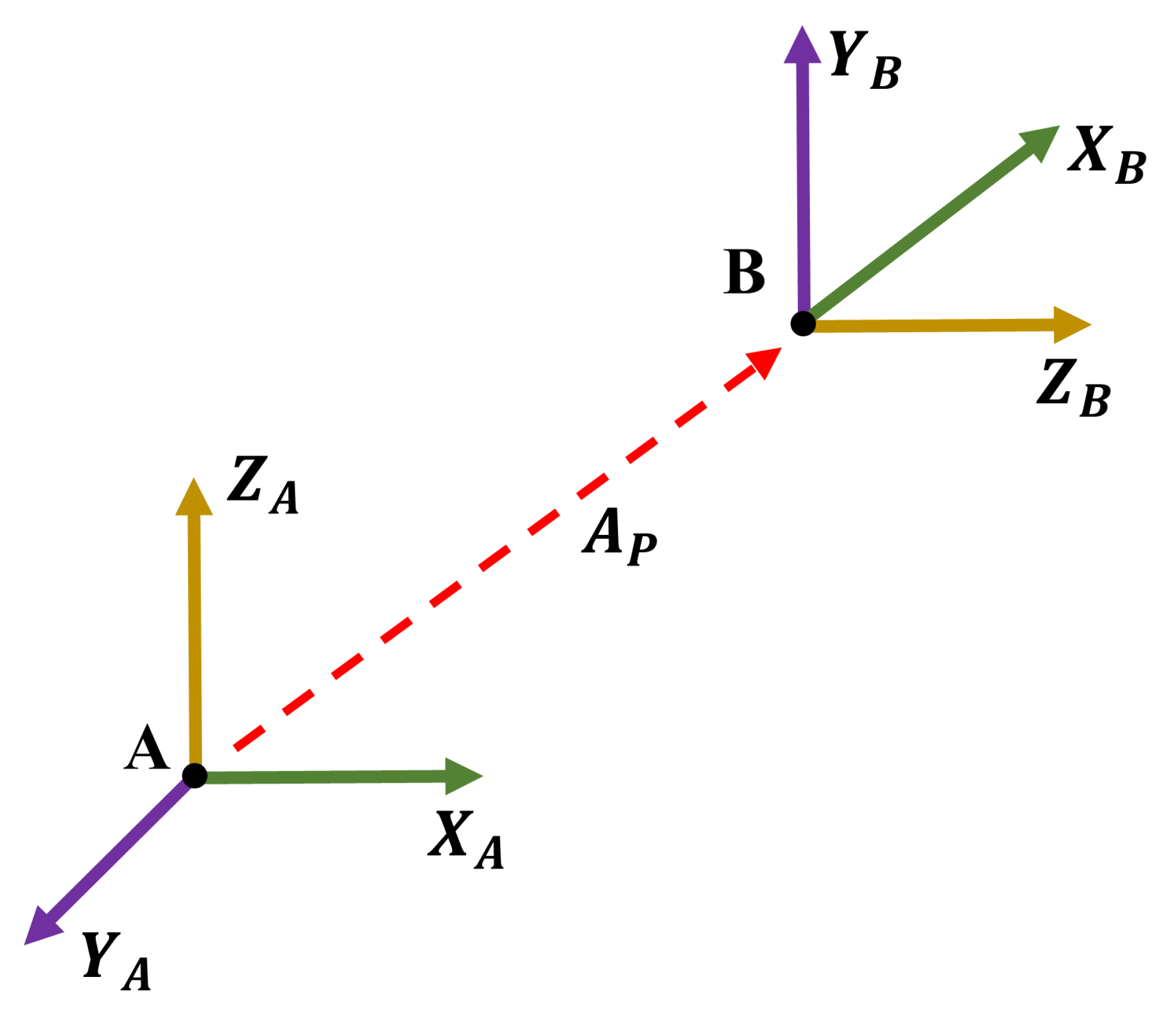
Frame
A is the base frame and frame
B is the transformed frame. Notice that frame
B has been translated and rotated.
is the translation of frame
A to frame
B and
is the rotation of frame
A to frame
B. Using the simple laws of trigonometry, the rotation of each axis is depicted with Equation (
2).
where
is the angle of rotation along the relevant axis and
R is the rotation matrix of that axis. Therefore, the complete relationship of frame
B to frame
A, i.e., the base frame, can be surmised with the transformation matrix seen in Equation (
3). The zeros and one are added to the matrix to make it a square matrix for ease in mathematical manipulation. Every successive frame can be similarly transformed from the base frame by simply multiplying its transformation matrix. A vector position
X in the frame of
B can be mapped with the base frame
A using Equation (
4).
To curb the complexity of devising such transformation matrices for a multi-faceted manipulator, Denavit–Hartenburg [
3] parameters are used, which stipulate that any serial manipulator can be described as a kinematic model by specifying four parameters for each link:
length of the link,
twist of the link,
offset of the link, and
angle of the joint.
With the advancement in technology arises the need to reduce time in the order of fractions of a second. Despite the ease of algebraic manipulation with the above-mentioned kinematic modelling, the increase in the number of links and their complexity brings forth numerical and geometric computations that require time and resources. It involves the solving of a series of simultaneous non-linear equations and, usually, multiple non-unique sets of solutions are obtained from one set of data.
Methods such as interval analysis [
4], dialytic and algebraic eliminitaion [
5], continuation [
6], and the Groebner basis approach [
7] have been used as numerical approaches to solve non-linear equations, but the problem of selecting an exact solution among several ones needs further manipulation. In literature, two schemes were adopted to find a unique solution, i.e., through auxiliary sensors and numerical procedures. The auxiliary sensors method [
8] has practical limitations, such as cost and measurement errors, while the numerical iteration method [
9] is sensitive to initial values and constraint equations. The problem of the planar cable-direct-driven robot architecture was solved through translational analytical method [
10]. The forward kinematic problem of a cablesuspended contour-crafting robot was solved through a simple numerical method [
11]. Despite how the kinematic modelling problem is identified, it still poses a challenge to find unique solutions. With the development of soft-computing-based methods, solving linear kinematic models in higher speeds has provided sufficient solutions, as compared to the traditional algebraic ones [
12]. To that effect, this paper proposes a soft-computing method, a Radial Basis Function Neural Network based on a meta-heuristic optimisation algorithm to model the forward kinematics of robotic manipulators.
2. Related Work
Soft computing aims at providing an understanding of the natural phenoma for algorithm development by attempting to mimic imprecision. Real-world applications contain uncertainties and imprecisions due to which a soft-computing-based mechanism is required that maps and caters to the unknown vagueness in the input-to-output transfer function. In the context of manipulators, algebraic elimination methods are time consuming and computationally expensive. In addition, the forward kinematics problem is not fully solved by giving a set of possible solutions, i.e., a unique solution is still a challenge. The identification of geometrical parameters is another complicated problem that requires some dedicated procedures and tools.
To circumvent such issues, many researchers have introduced connectionist networks. The array of interconnected neurons serve as a means to map the forward kinematic task. For example, a holographic neural network (HNN) was proposed in [
13] to model a planar 3-Degrees of Freedom (DOF) manipulator. With the use of a multi-layer perceptron, a kinematic model for the HEXA robot was generated in [
14]. In [
15], the authors aimed at learning the forward kinematic behaviour of a hybrid parallel–serial structure-based manipulator, the training of which was conducted by a meta-heuristic algorithm, i.e., a Particle Swarm Optimiser (PSO). For obtaining approximate but accurate solutions of forward kinematic modelling for the Stewart platform, a popular parallel robots variant, a classic machine learning technique, i.e., support vector machine, was used in [
16]. The kinematic problem of manipulators was addressed as a supervised learning problem by [
2], who proposed a Multi-Layer Perceptron (MLP) architecture which was tested on a simulated robot for the 7-DOF Sawyer Robotic Arm. In [
17], an Artificial Neural Network (ANN) was used to control a 4-DOF robotic arm with a 2-DOF end effector attached on bomb disposal robots to an error accuracy of about 5 mm. A neural network model using the back-propagation algorithm was used on a Stewart platform to solve the problem of asymmetric payload [
18]. An MLP with one input layer, five hidden layers, and a single output layer was used to solve the form of cable robots’ forward kinematics in [
19]. A popular machine learning technique, Support Vector Regression (SVR), was modelled on the Robotic Research Arm K-1207 to mimic the forward kinematic behaviour [
20,
21].
However, while the literature shows that much focus is being placed on this research field, the problem of highly accurate and generalised network models still persists, especially for engineering design problems for robotic manipulators such as the machining of aircraft parts or automotive manufacturing. This paper proposes a novel network model that can provide end-effector position and solve the forward kinematic issue for a 3-DOF manipulator.
3. Methodology
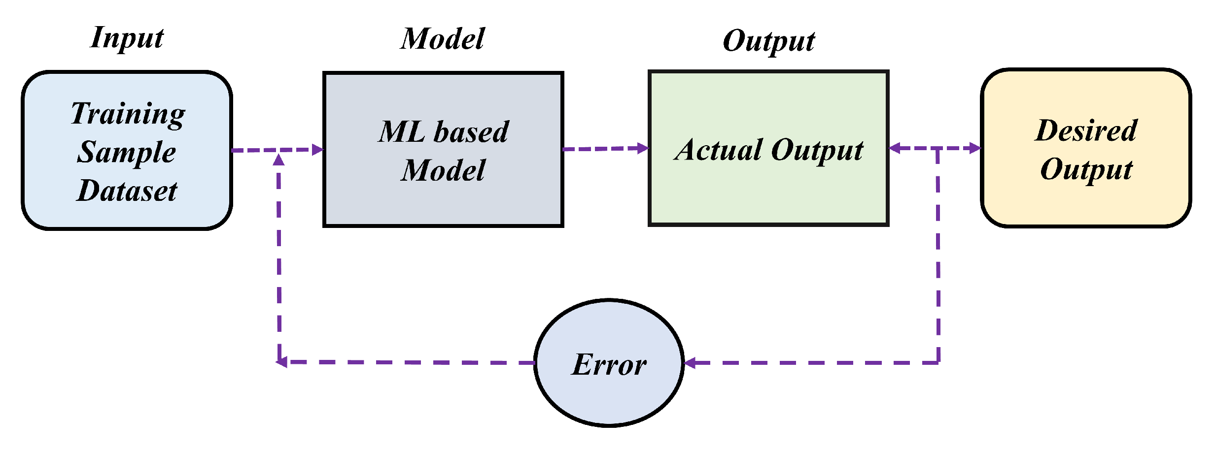
It can be devised that the kinematic estimation of an end-effector pose can be computed with the help of a supervised Machine Learning (ML) algorithm. The ML-based architecture that shall be used for such computation needs to be pre-trained from the training samples made from measurements. Once the training has been accomplished to a significant level of accuracy, it can be used for end-effector positioning.
Figure 3 conceptualises the training process that is to be conducted offline with a dataset of labelled training samples. For the purpose of this study, a 3-DOF robotic manipulator with three revolute type joints is to be used for data sampling. Once the dataset has been generated, it will be fed into a Radial Basis Function Neural Network architecture, tuned with the help of a novel Cooperative Search Optimisation Algorithm. Finally, the output of the model will be compared with the the true values of the robotic end-effector position and the relevant errors will be fed back into the network for to update parameters and reduce errors. This section discusses how each of the processes mentioned are developed.
3.1. Dataset Preparation
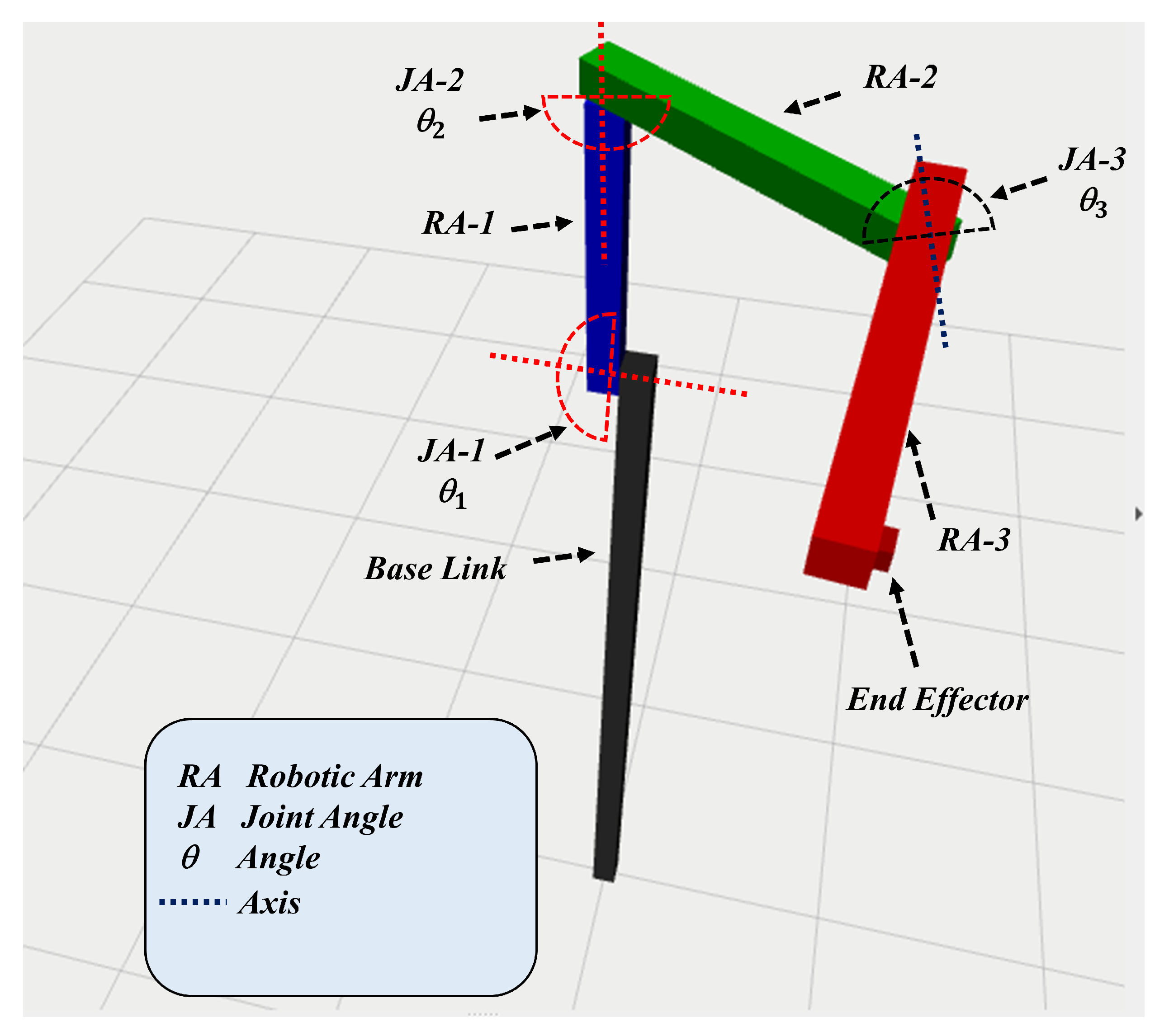
First and foremost, the key goal is to prepare a dataset on which the proposed model is to be trained. Therefore, the cartesian coordinates (X, Y, Z) of the end-effector position are needed with respect to the joint angle of the 3-DOF robotic manipulator. An inherent complication with this approach is that the Cartesian coordinates must be obtained from an external sensor, and most mechanical manipulators possess only internal sensors. However, if the geometric characteristics of the robot are known, then the training dataset can be also generated from a simulated kinematic model of the robot.
To accomplish the proposed task of simulating the kinematic model of the robot, the Robot Operating System (ROS) was employed. ROS is an open-source, meta-operating system that is used for robot research and development. A 3-DOF robot with revolute joints was created in ROS.
Figure 4 shows the visualisation of the robot in RViZ [
22].
The robot’s state publisher tool is utilised to publish the state of the robot, i.e., the transformation of the links, joints, and Cartesian positions. The tool basically broadcasts the state of the robot as an ROS node. The model was constructed by reverse-engineering the geometrical properties of the physical robot on a Unified Robotic Description Format (URDF) model file. With the help of the URDF description and the joint states that publish the joint positions, the manipulator was simulated, the joint angles of each link, and the Cartesian coordinate of the end-effector were sampled to create a dataset of 1000 randomly generated entries. The sample dataset created can be seen in
Table 1.
If the inverse mapping of the end-effector position to the joint angles’ vector is unique, then the inverse kinematic model is considered to be well-posed. However, if the mapping has many solutions, i.e., has many angle vectors that can obtain the desired end-effector position, or if it has no solution, i.e., singularities, then the inverse kinematic model is considered to be ill-posed. Singularities can be of two kinds: the first is where the robotic manipulator is desired to bring the end-effector position outside of the manipulator workspace, and second is caused by an alignment of the robot’s axes in space, leaving the actual joint location indeterminate. To cater for these problems that will cause inefficiencies for the training model, the dataset has been preprocessed, i.e., the non-existent data samples have been removed, leaving the final trainable dataset of 100 distinct entries.
3.2. ML-Based Architecture
This section provides an overview of the network model and the novel method used to tune the model for the robotic manipulator.
3.2.1. Radial Basis Function Neural Network (RBFNN)
Radial Basis Function (RBF) networks are a type of artificial neural network commonly used for function approximation problems. RBFNN is a popular alternative to the Feed-Forward Back-Propagation Neural Network (FFBPNN), which was presented by Broomhead and Lowe [
23]. The weights and activation of a transfer function
F provided for the units determine the network’s behaviour. The output of a processing node is determined by activation functions, which are mathematical formulas. By applying
F to the output value, the activation function maps the sum of weighted values provided to them, which is then “fired” onto the next layer.
Linear Function (LF), Threshold Function (TF), Sigmoid Function (SF), and Radial Basis Function (RBF) are four types of transfers or activation functions [
24]. RBFs are a type of activation function that consists of a collection of basis functions, one for each dataset. RBF takes the following broad form, as depicted in Equation (
5):
where
G is a nonlinear symmetric radial function (kernel);
X is the input pattern; and
is the function’s centre. The RBF’s output is also symmetric to the related centre, which is a significant feature. As a result,
can be considered a linear combination of all the basis functions’ outputs:
There are several common types of Radial Basis Functions, as represented in
Table 2.
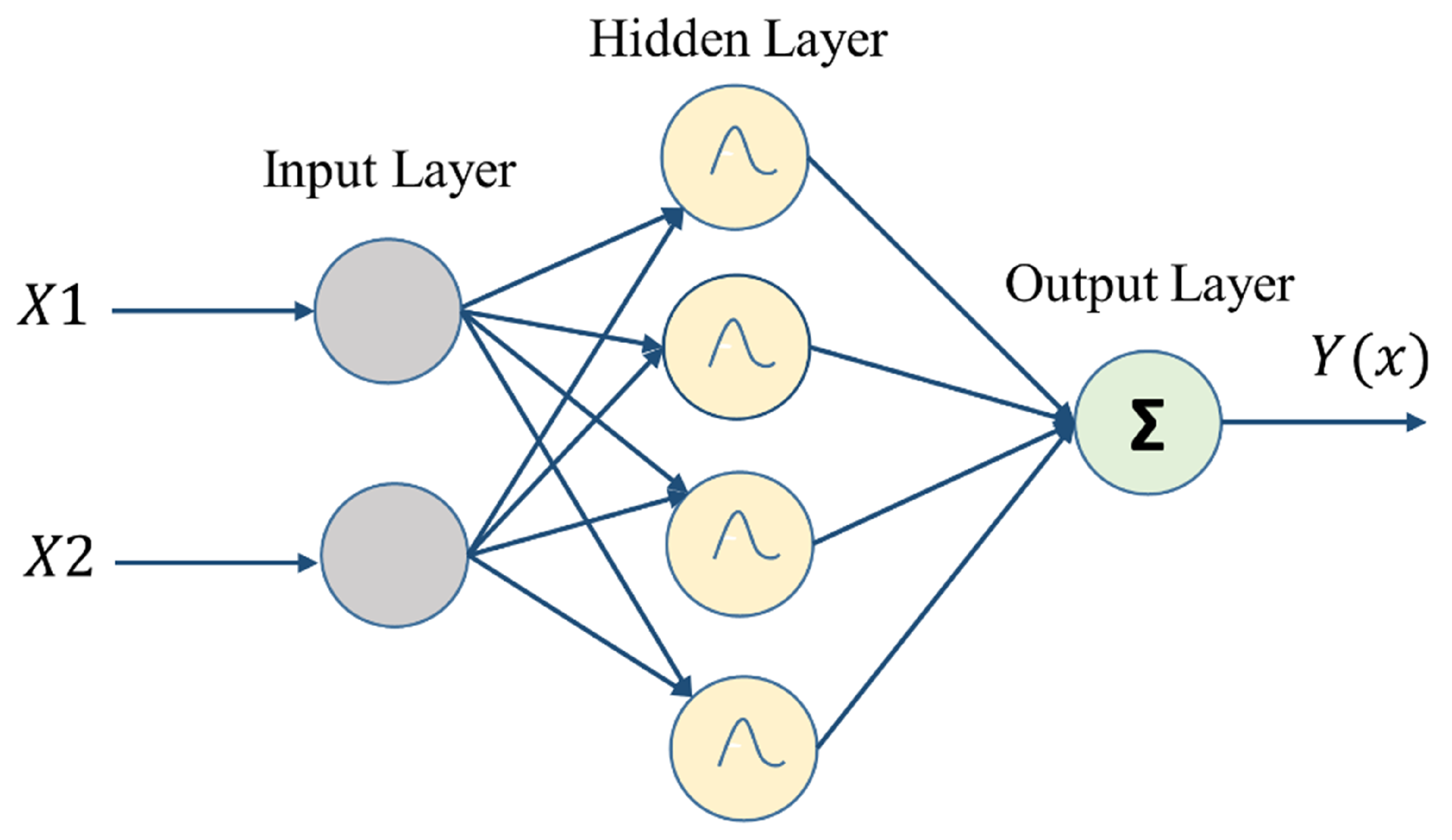
RBFNN is a feed-forward NN model, as shown in
Figure 5, in which the activation function of the hidden unit is determined by the distance between the input vector and a prototype vector. The proposed RBFNN consists of the input layer, the hidden layer, and the output layer. The input layer consists of two neurons that take a manipulator’s joint angular position as an input and compute the Cartesian coordinates of the end-effector as the output. The input layer transmits the net input and output data to the next layer as:
where
and
are the mean and the standard deviation of the Gaussian function, respectively. The output layer has a single neuron with a node
. The output signal is computed by making a summation of incoming signals.
where
is the weight(s) that connects the hidden and output layers.
3.2.2. Cooperative Search Optimisation Algorithm (CSOA)
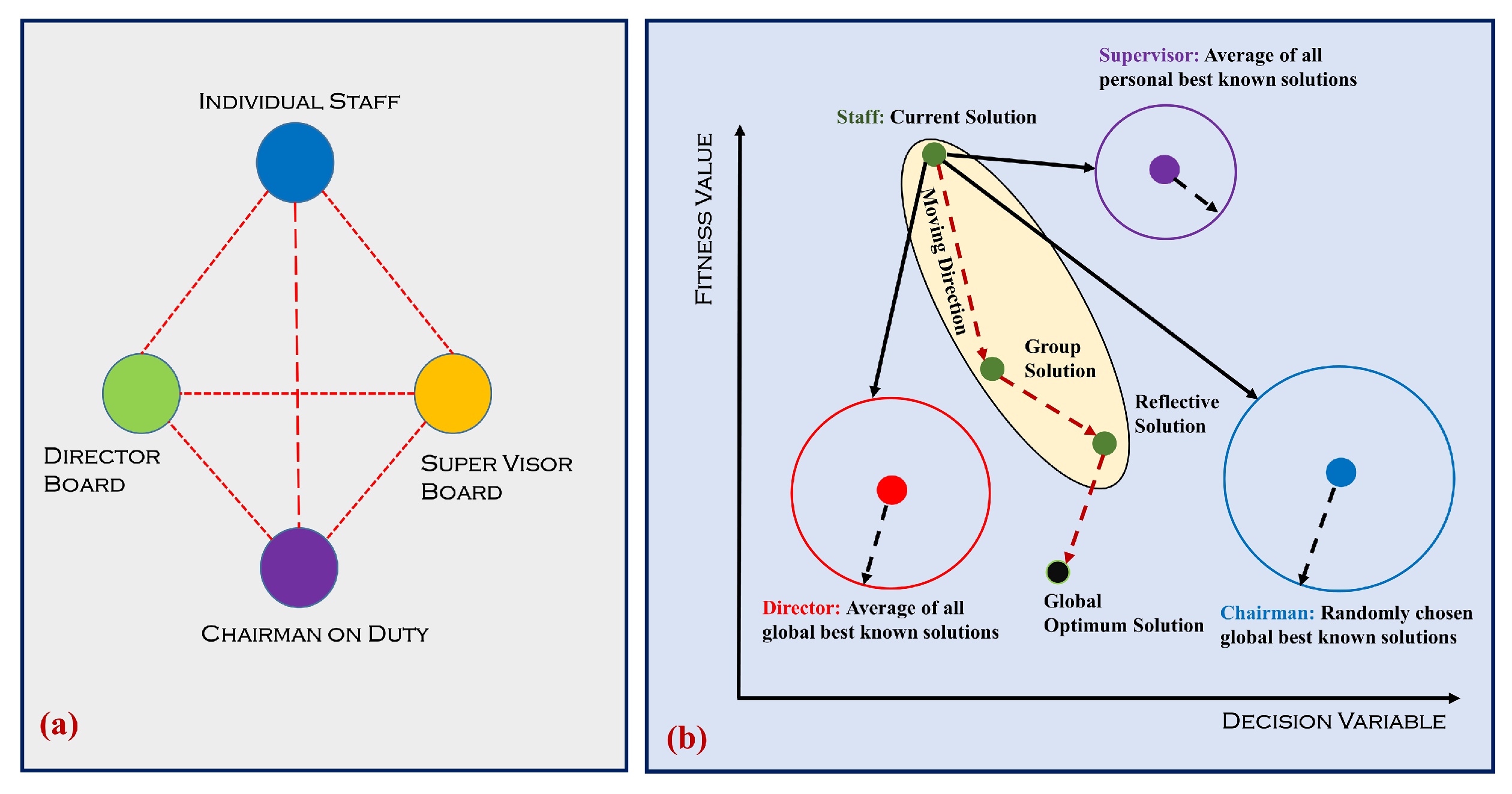
The model of an enterprise is mimicked and inspired by the Cooperative Search Optimisation Algorithm (CSOA) [
25], in which the staff represents the solutions and the performance of every staff member represents the fitness function value. The sketch of a team relationship is shown in
Figure 6. Personal best solutions can be represented as the board of supervisors while the board of directors represents the number of global best solutions. Chairmen can be selected from the board of directors. The position updates of particles for high-quality solutions utilise different operators. The detailed mathematical model of CSOA is presented below, in the form of different stages.
Like every meta-heuristic algorithm, CSOA also initialises the solutions randomly in the whole search space, using Equation (
11).
where
is the randomly generated solution,
is the function used to generate solutions within the maximum
and minimum value
of the search space. After calculating the fitness value of every solution, the elite vector M is created.
- b.
Team Communication Phase:
Each staff member can obtain a new message by sharing information with a chairperson, the board of directors, and the supervisors. The mathematical model of the team communication phase is presented in Equation (
12).
where
A represents the chairman’s knowledge, and
B represents the knowledge of the board of directors, which is the mean knowledge calculated from
M.
C represents the knowledge of supervisors, which is the mean knowledge calculated from
I.
is the updated position particle,
is the global best value,
is the personal best value,
I represents the vector of personal best group, and
M represents the vector of elite solutions. The
and
are the tuning parameters, which need to be adjusted for the required application.
- c.
Reflective Learning Phase:
Another way for staff to gain knowledge is by summing their own experiences in the opposite direction. The mathematical model for the reflective learning phase is shown below:
where
is the
value of the reflective solution at the
cycle. The pseudo-code of the CSOA is shown in Algorithm 1.
| Algorithm 1: Pseudo-code for CSOA algorithm. |
Data: Random data in search space Result: Output the best final solution Initialise objective function and random population on search space; Evaluate the fitness of all particles and create I and M vectors; whiletermination criteria not metdo ![Robotics 11 00043 i001]() end |
4. Results
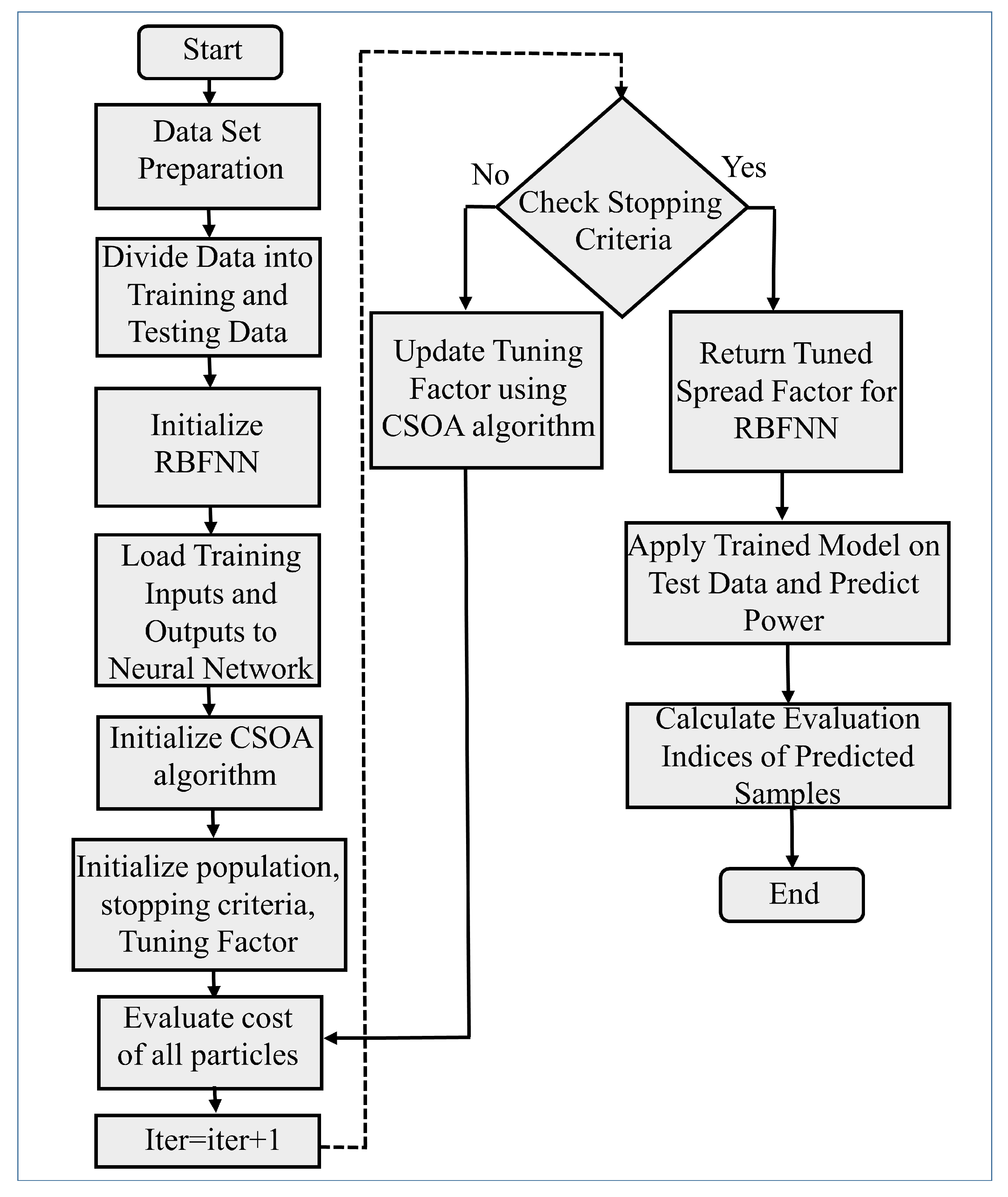
RBFNN suffers from low prediction accuracy if the parameters, i.e., the
smoothing parameter with the number of neurons in RBFNN, do not tune well. For effective training and testing, these parameters need to be optimally tuned. In this paper, CSOA is used to tune these parameters, and forward kinematic prediction is performed. The flow chart for the training of RBFNN using CSOA is shown in
Figure 7. Trained models are then tested on the test data and the performance evaluation is performed.
First, the dataset is prepared, which is then divided into training and testing data with a 65% to 35% ratio. After that, the RBFNN network is initialised and the train dataset is fed into the RBFNN network. To effectively tune the smoothing parameter, the Cooperative Search Optimisation Algorithm is initialised, which will update the value of the smoothing parameter to obtain the best training accuracy.
This section discusses the proposed model for the forward kinematics prediction, and after that, a comparison of the proposed techniques is made between GWO-RBFNN and PSO-RBFNN. A statistical analysis is presented to check the sensitivity of the proposed technique. To ensure a fair comparison, the number of iterations for the meta-heuristic algorithm is set to 50 and the multi-agents that will converge toward the optimum solution is set to 50 as well. The parameters set for the algorithm are shown in
Table 3. The value of the control parameters were chosen according to the literature presented for the algorithms of PSO and GWO.
4.1. CSOA-RBFNN Model
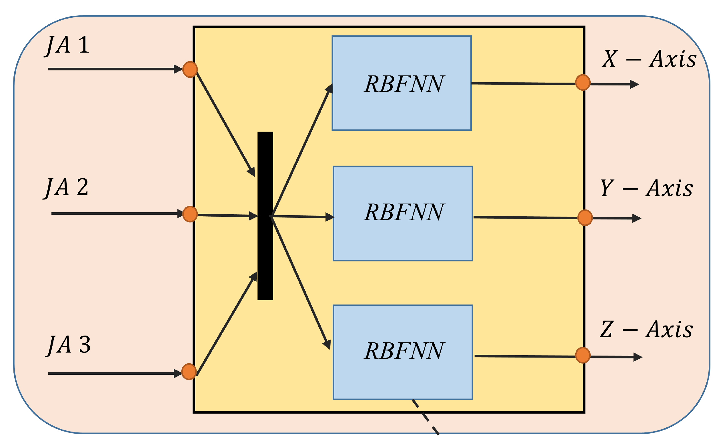
The smoothing parameter is an important parameter to tune in RBFNN, which is condnucted by the CSOA. In this work, three different RBFNN networks are used for the prediction of each axis position. So, the smoothing parameter needs to be tuned for each axis dataset. The structure of the RBFNN used for the prediction of forward kinematics is shown in
Figure 8. The cost function used is the Normalised Mean Square Error (NMSE).
4.1.1. X-axis Prediction Results
In regression problems, the relative error, Normalised Mean Square Error, and the Mean Absolute Error are the best indices to measure the performance of the prediction.
Figure 9 shows the comparison of predictions of the
x-axis position, while the relative error comparison is shown in
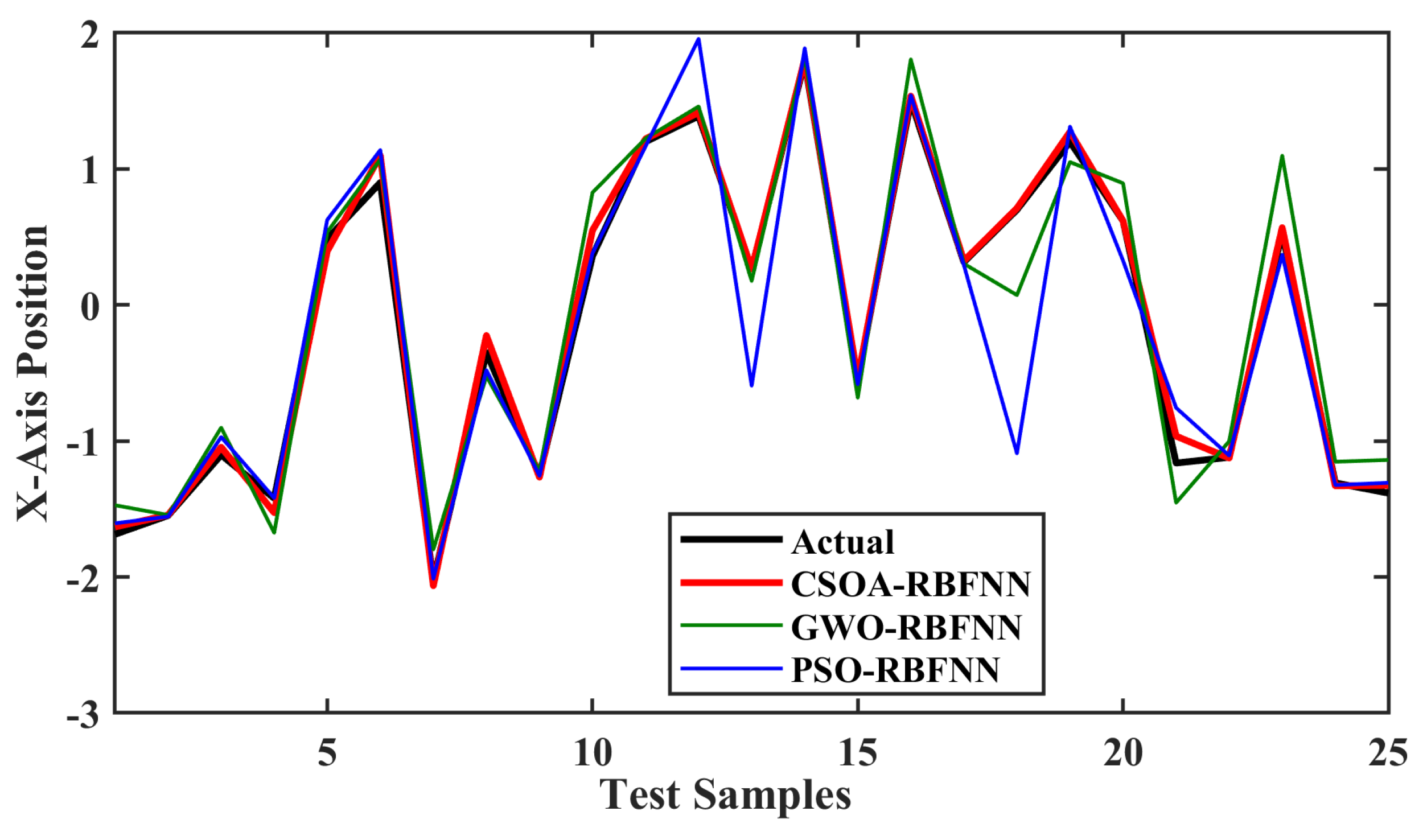
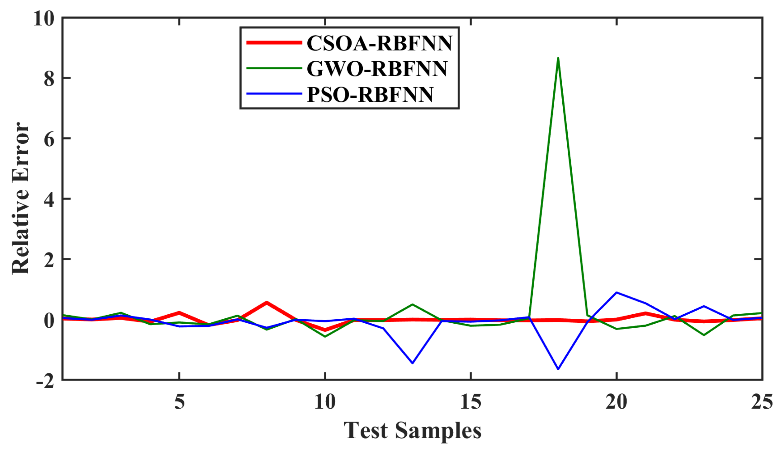
Figure 10. The prediction curve shows that CSOA-RBFNN has better prediction accuracy than GWO-RBFNN and PSO-RBFNN. The relative error curve comparison also shows that the CSOA-RBFNN has a value close to zero, which is less than GWO-RBFNN and PSO-RBFNN.
As presented in
Table 4, the optimal value of the smoothing factor achieved by CSOA-RBFNN, GWO-RBFNN, and PSO-RBFNN are 2.2, 2.7, and 2.9, respectively. The best cost during training, achieved by CSOA-RBFNN, is 0.0048; GWO-RBFNN is 0.0412 and PSO-RBFNN is 0.2230.
Table 5 shows the statistical analysis of the prediction made by the techniques on the test data. The Mean Relative Error achieved by CSOA-RBFNN is 0.0098; GWO-RBFNN is 0.3015 and PSO-RBFNN is 0.856. The statistical analysis shows that the CSOA-RBFNN achieved high prediction accuracy, as compared to GWO-RBFNN and PSO-RBFNN, for the
x-axis.
4.1.2. Y-axis Prediction Results
Figure 11 shows the comparison of predictions of the
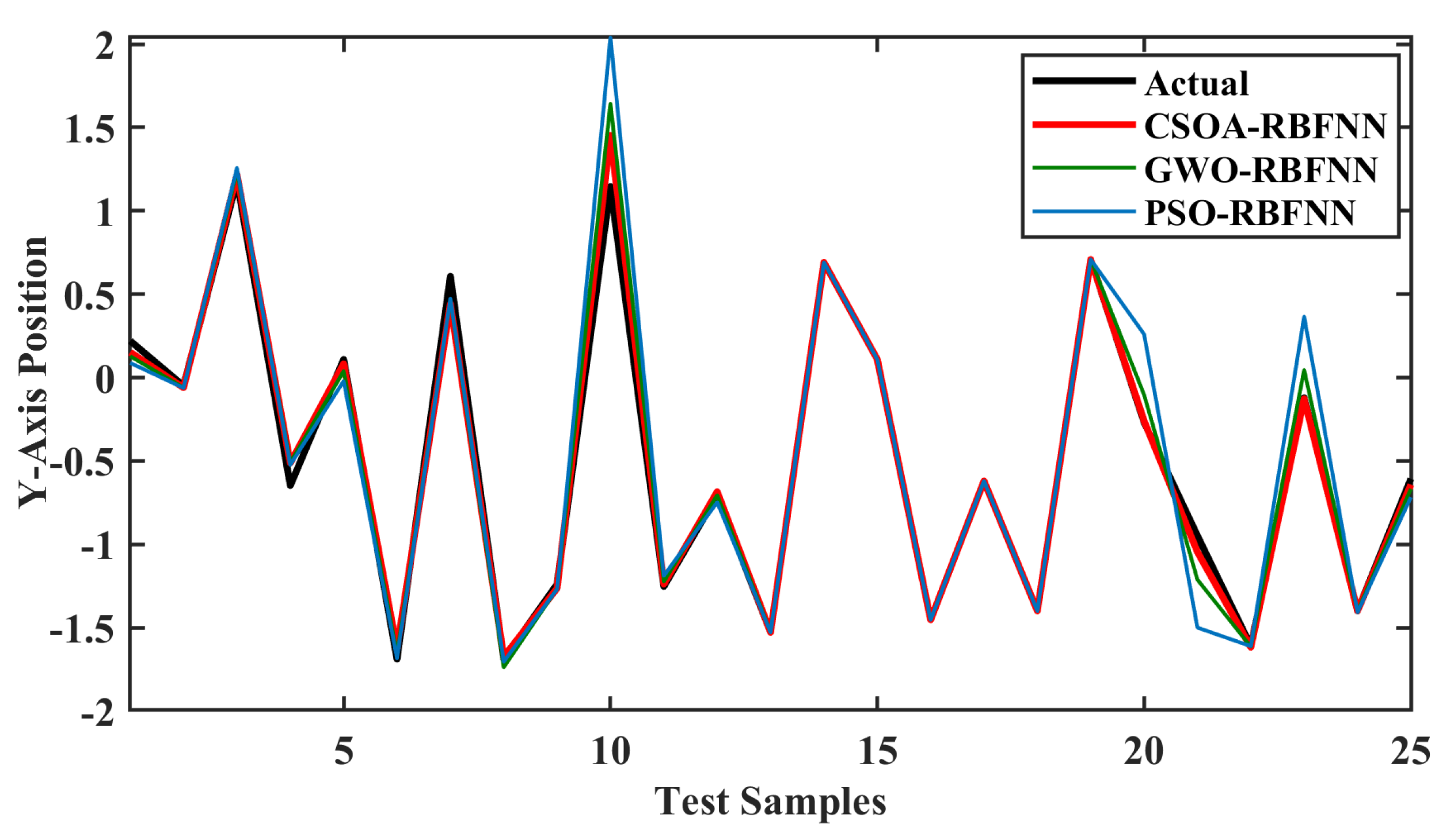
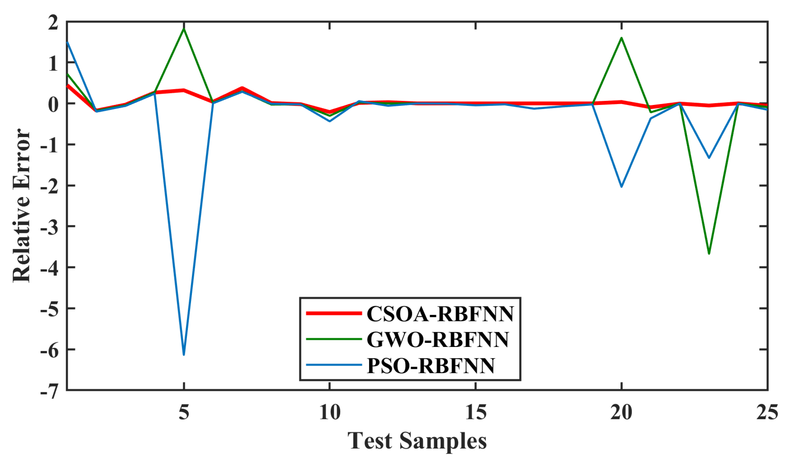
y-axis position, while the relative error comparison is shown in
Figure 12. The prediction curve shows that CSOA-RBFNN has better prediction accuracy than GWO-RBFNN and PSO-RBFNN. The relative error curve comparison also shows that the CSOA-RBFNN has a value close to zero, which is less than GWO-RBFNN and PSO-RBFNN.
As presented in
Table 6, the optimal value of the smoothing factor achieved by CSOA-RBFNN, GWO-RBFNN, and PSO-RBFNN are 1.9, 2.1, and 2.5, respectively. The best cost during training, achieved by CSOA-RBFNN, is 0.0083; GWO-RBFNN is 0.0225 and PSO-RBFNN is 0.0861.
Table 7 shows the statistical analysis of the prediction made by the techniques on the test data. The Mean Relative Error achieved by CSOA-RBFNN is 0.0355; GWO-RBFNN is 0.086 and PSO-RBFNN is 0.3616. The statistical analysis shows that the CSOA-RBFNN achieved high prediction accuracy, as compared to GWO-RBFNN and PSO-RBFNN, for the
y-axis. Thus, the CSOA-RBFNN has 90% less Mean Relative Error, 89.6% less NMSE, and 81.5% less MAE, as compared to the competing techniques, in its prediction of the
y-axis.
4.1.3. Z-axis Prediction Results
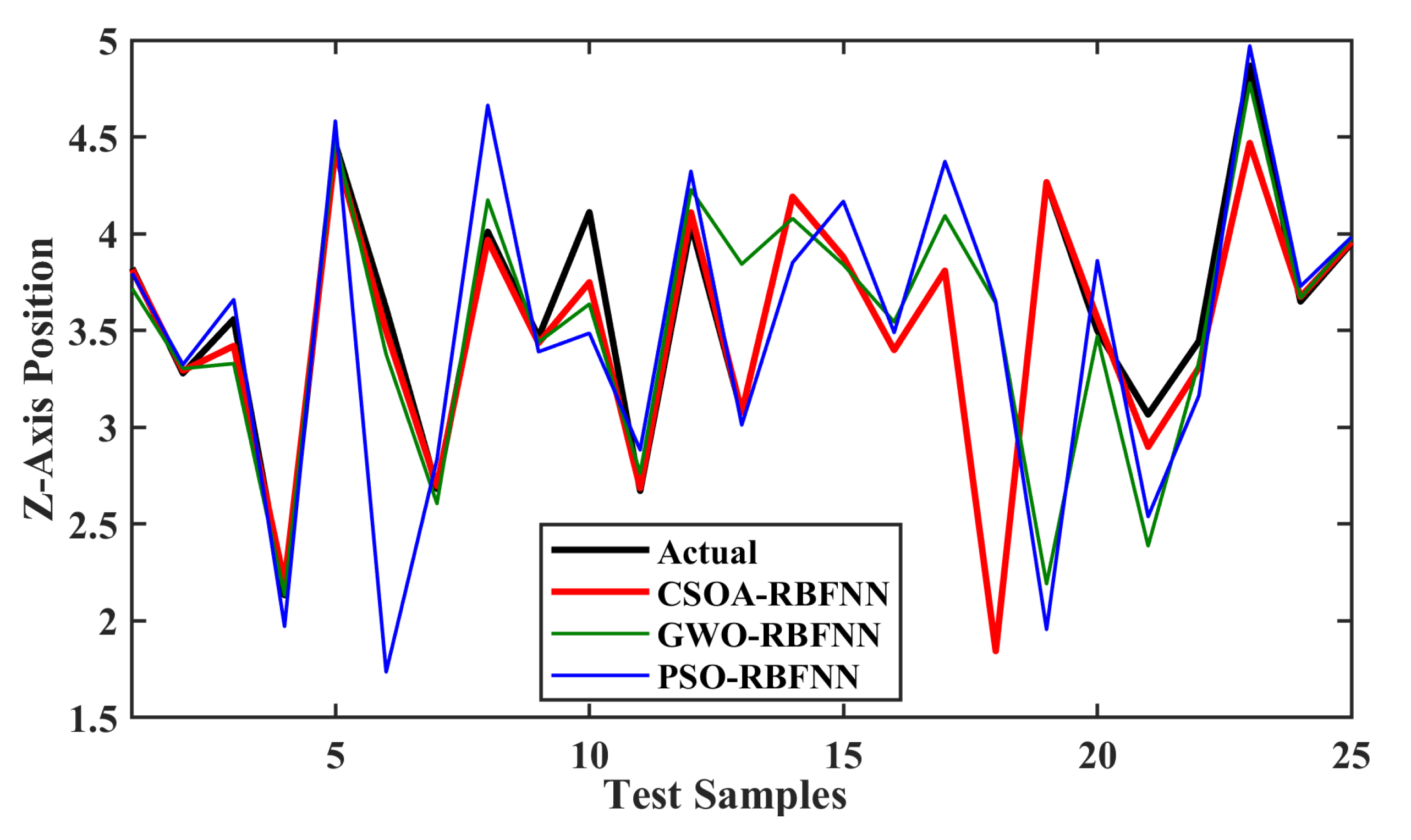
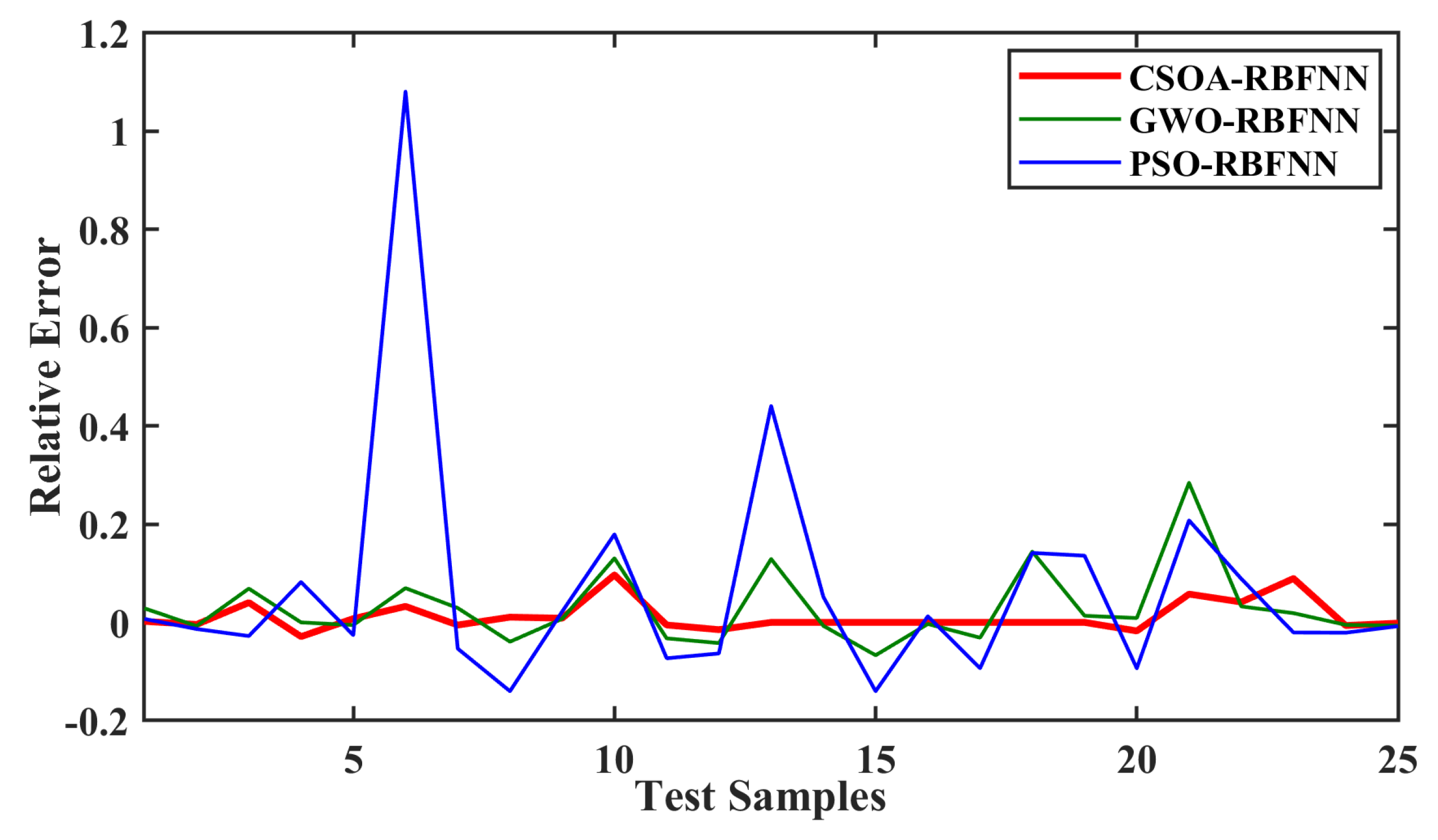
Figure 13 shows the comparison of predictions of the
z-axis position, while the relative error comparison is shown in
Figure 14. The prediction curve shows that CSOA-RBFNN has better prediction accuracy than GWO-RBFNN and PSO-RBFNN. The relative error curve comparison also shows that the CSOA-RBFNN has a value close to zero, which is less than GWO-RBFNN and PSO-RBFNN.
As presented in
Table 8, the optimal value of the smoothing factor achieved by CSOA-RBFNN, GWO-RBFNN, and PSO-RBFNN are 1.4, 2.1, and 7.2, respectively. The best cost during training, achieved by CSOA-RBFNN, is 0.0321; GWO-RBFNN is 0.1426 and PSO-RBFNN is 0.4307.
Table 9 shows the statistical analysis of the prediction made by the techniques on the test data. The Mean Relative Error achieved by CSOA-RBFNN is 0.0121; GWO-RBFNN is 0.0287 and PSO-RBFNN is 0.0671. The statistical analysis shows that the CSOA-RBFNN achieved high prediction accuracy, as compared to GWO-RBFNN and PSO-RBFNN, for the
z-axis.
4.2. Comparative Study
This section propounds the comparison of the proposed RBFNN-CSOA technique with the previously established soft-computing techniques, as postulated in the Related Work section, i.e., the proposed model is compared with an ANN network and a Support Vector Regression model.
An ANN model is created with a single 3-neuron input layer for the joint angles, a hidden layer of 10 neurons, and a single output layer. The models are compared on each axis on the pre-processed dataset. The comparative analysis is shown in
Table 10.
The results for Mean Relative Error, NMSE, and MAE show the superiority and accuracy of the proposed model over the SVR and ANN models. In cases where the number of features for each data point exceeds the number of training data samples, the SVR model underperforms while the back-propagation-based ANN model faces high time complexity and vanishing gradient problems with complex, high-variance datasets. The usage of the CSOA meta heuristic algorithm has better global minima-finding capabilities than its predecessor techniques for forward kinematic modelling.
5. Discussion
Formulating the suitable kinematics models for a robot mechanism is very crucial for analysing the behaviour of industrial manipulators. Models presented in most of the literature is accomplished using traditional geometric manipulation and/or the use of transformation matrix standards such as the Denavit–Hartenburg (DH) table. Such transformations present problems of computation and time complexity when high Degrees of Freedom (DOFs) of robotic manipulators are introduced.
To circumvent such issues, the use of soft-computing techniques is introduced. The proposed model, CSOA-RBFNN, is compared with previous studies of soft-computing techniques and is also compared with other meta-heuristic algorithms to show the efficacy of the model presented in the manuscript. The simulation of a 3-DOF robotic manipulator is created in ROS-RVIZ, and a dataset is generated with 1000 random-position samples of the manipulator.
Ill-posed kinematic modelling and singularities are created during the random sampling processes for the dataset-generation process. To ensure the neural network is trained accurately, redundant data needs to be removed from the dataset. Therefore, the dataset is preprocessed to 100 trainable entries. Finally, the dataset is then split in a 65/35 ratio for training and testing sets.
A comparative analysis is performed with previous soft-computing models presented in the literature. Secondly, a comparison of meta-heuristic techniques, both traditional and new, for training a Radial Basis Function Neural Network is also postulated. The results show that the proposed technique has better accuracy and relative errors. The use of such techniques puts forward a better solution to kinematic modelling than previously articulated techniques.
6. Conclusions and Future Work
Exact algebraic mapping of end-effector position in Cartesian space entails high computational weight and time lag when there are many Degrees of Freedom (DOFs) for the manipulator. This paper proposed a model for the forward kinematic estimation of robotic manipulators using soft-computing techniques. A Radial Basis Function Neural Network (RBFNN) tuned with the Cooperative Search Optimisation Algorithm (CSOA) was used to determine the end-effector position of a 3-DOF robotic manipulator. Simulations of the robotic manipulator, to create an angle joint to end-effector position dataset, were conducted on the Robot Operating System (ROS). The CSOA-RBFNN model was trained on 65% of the dataset, while the remainder was used for testing. The metrics used for the analysis of the efficacy of the technique are optimal spread value, best cost, and runtime for the training of the model, and Mean Relative Error, Normal Mean Square Error, and Mean Absolute Error for the testing of the model. A comparative study of the model has also been carried out with an artificial neural network, Support Vector Regression (SVR) model, and other meta-heuristic techniques, i.e., Particle Swarm Optimisation (PSO)-based RBFNN and Grey Wolf Optimiser (GWO)-based RBFNN models. The results show the superiority of this paper’s technique, and that it is a better approach for solving kinematic estimation problems in real-world applications.
While the modelling was performed in a pre-processed dataset generated from a simulation, future work includes training the model and performing the validation process in real time. Secondly, the venue of inverse kinematic modelling also presents a way forward, although singularities and nonlinearities make the problem more difficult to solve.
Author Contributions
Conceptualisation, S.K.R.M. and M.H.Z.; methodology, S.K.R.M. and M.H.Z.; software, S.K.R.M. and M.H.Z.; validation, F.S.; formal analysis, S.K.R.M. and M.H.Z.; investigation, F.S.; resources, F.S.; writing—original draft preparation, S.K.R.M., M.H.Z. and F.S.; writing—review and editing, F.S.; supervision, F.S.; funding acquisition, F.S. All authors have read and agreed to the published version of the manuscript.
Institutional Review Board Statement
Not applicable.
Informed Consent Statement
Not applicable.
Conflicts of Interest
The authors declare no conflict of interest. The funders had no role in the design of the study; in the collection, analyses, or interpretation of data; in the writing of the manuscript, or in the decision to publish the results.
References
- Vukobratović, M. General Introduction to Robots. In Introduction to Robotics; Springer: Berlin/Heidelberg, Germany, 1989; pp. 1–18. [Google Scholar]
- Theofanidis, M.; Sayed, S.I.; Cloud, J.; Brady, J.; Makedon, F. Kinematic estimation with neural networks for robotic manipulators. In Proceedings of the International Conference on Artificial Neural Networks, Rhodes, Greece, 4–7 October 2018; Springer: Berlin/Heidelberg, Germany, 2018; pp. 795–802. [Google Scholar]
- Corke, P.I. A simple and systematic approach to assigning Denavit—Hartenberg parameters. IEEE Trans. Robot. 2007, 23, 590–594. [Google Scholar] [CrossRef] [Green Version]
- Merlet, J.P. Solving the forward kinematics of a Gough-type parallel manipulator with interval analysis. Int. J. Robot. Res. 2004, 23, 221–235. [Google Scholar] [CrossRef]
- Lee, T.Y.; Shim, J.K. Improved dialytic elimination algorithm for the forward kinematics of the general Stewart—Gough platform. Mech. Mach. Theory 2003, 38, 563–577. [Google Scholar] [CrossRef]
- Raghavan, M. The Stewart Platform of General Geometry Has 40 Configurations. J. Mech. Des. 1993, 115, 277–282. [Google Scholar] [CrossRef]
- Gan, D.; Liao, Q.; Dai, J.S.; Wei, S.; Seneviratne, L. Forward displacement analysis of the general 6—6 Stewart mechanism using Gröbner bases. Mech. Mach. Theory 2009, 44, 1640–1647. [Google Scholar] [CrossRef]
- Wang, Y. A direct numerical solution to forward kinematics of general Stewart—Gough platforms. Robotica 2007, 25, 121–128. [Google Scholar] [CrossRef]
- Baron, L.; Angeles, J. The direct kinematics of parallel manipulators under joint-sensor redundancy. IEEE Trans. Robot. Autom. 2000, 16, 12–19. [Google Scholar] [CrossRef]
- Williams Ii, R.L.; Gallina, P. Translational planar cable-direct-driven robots. J. Intell. Robot. Syst. 2003, 37, 69–96. [Google Scholar] [CrossRef]
- Bosscher, P.; Williams, R.L., II; Bryson, L.S.; Castro-Lacouture, D. Cable-suspended robotic contour crafting system. Autom. Constr. 2007, 17, 45–55. [Google Scholar] [CrossRef]
- El-Sherbiny, A.; Elhosseini, M.A.; Haikal, A.Y. A comparative study of soft computing methods to solve inverse kinematics problem. Ain Shams Eng. J. 2018, 9, 2535–2548. [Google Scholar] [CrossRef]
- Boudreau, R.; Levesque, G.; Darenfed, S. Parallel manipulator kinematics learning using holographic neural network models. Robot. Comput.-Integr. Manuf. 1998, 14, 37–44. [Google Scholar] [CrossRef]
- Dehghani, M.; Ahmadi, M.; Khayatian, A.; Eghtesad, M.; Farid, M. Neural network solution for forward kinematics problem of HEXA parallel robot. In Proceedings of the 2008 American Control Conference, Seattle, WA, USA, 11–13 June 2008; IEEE: Piscataway, NJ, USA, 2008; pp. 4214–4219. [Google Scholar]
- Kang, R.; Chanal, H.; Bonnemains, T.; Pateloup, S.; Branson, D.T.; Ray, P. Learning the forward kinematics behavior of a hybrid robot employing artificial neural networks. Robotica 2012, 30, 847–855. [Google Scholar] [CrossRef]
- Morell, A.; Acosta, L.; Toledo, J. An artificial intelligence approach to forward kinematics of Stewart platforms. In Proceedings of the 2012 20th Mediterranean Conference on Control & Automation (MED), Barcelona, Spain, 3–6 July 2012; IEEE: Piscataway, NJ, USA, 2012; pp. 433–438. [Google Scholar]
- Ligutan, D.D.; Abad, A.C.; Dadios, E.P. Adaptive robotic arm control using artificial neural network. In Proceedings of the 2018 IEEE 10th International Conference on Humanoid, Nanotechnology, Information Technology, Communication and Control, Environment and Management (HNICEM), Baguio City, Philippines, 29 November–2 December 2018; IEEE: Piscataway, NJ, USA, 2018; pp. 1–6. [Google Scholar]
- Faraji, H.; Rezvani, K.; Hajimirzaalian, H.; Sabour, M.H. Solving the Forward Kinematics Problem in Parallel Manipulators Using Neural Network. In Proceedings of the 2017 the 5th International Conference on Control, Mechatronics and Automation, Edmonton, AB, Canada, 11–13 October 2017; pp. 23–29. [Google Scholar]
- Ghasemi, A.; Eghtesad, M.; Farid, M. Neural network solution for forward kinematics problem of cable robots. J. Intell. Robot. Syst. 2010, 60, 201–215. [Google Scholar] [CrossRef]
- Morell, A.; Tarokh, M.; Acosta, L. Solving the forward kinematics problem in parallel robots using Support Vector Regression. Eng. Appl. Artif. Intell. 2013, 26, 1698–1706. [Google Scholar] [CrossRef]
- Morell, A.; Tarokh, M.; Acosta, L. Inverse kinematics solutions for serial robots using support vector regression. In Proceedings of the 2013 IEEE International Conference on Robotics and Automation, Karlsruhe, Germany, 6–10 May 2013; IEEE: Piscataway, NJ, USA, 2013; pp. 4203–4208. [Google Scholar]
- Hernandez-Mendez, S.; Maldonado-Mendez, C.; Marin-Hernandez, A.; Rios-Figueroa, H.V.; Vazquez-Leal, H.; Palacios-Hernandez, E.R. Design and implementation of a robotic arm using ROS and MoveIt! In Proceedings of the 2017 IEEE International Autumn Meeting on Power, Electronics and Computing (ROPEC), Zihuatanejo, Mexico, 4–6 November 2015; IEEE: Piscataway, NJ, USA, 2017; pp. 1–6. [Google Scholar]
- Broomhead, D.S.; Lowe, D. Radial Basis Functions, Multi-Variable Functional Interpolation and Adaptive Networks. Technical Report. Royal Signals and Radar Establishment Malvern (United Kingdom). 1988. Available online: https://apps.dtic.mil/sti/citations/ADA196234 (accessed on 27 March 2022).
- Zadeh, M.R.; Amin, S.; Khalili, D.; Singh, V.P. Daily outflow prediction by multi layer perceptron with logistic sigmoid and tangent sigmoid activation functions. Water Resour. Manag. 2010, 24, 2673–2688. [Google Scholar] [CrossRef]
- Feng, Z.K.; Niu, W.J.; Liu, S. Cooperation search algorithm: A novel metaheuristic evolutionary intelligence algorithm for numerical optimization and engineering optimization problems. Appl. Soft Comput. 2021, 98, 106734. [Google Scholar] [CrossRef]
Figure 1.
Types of joints: (a) articulated manipulator, (b) spherical manipulator, (c) SCARA manipulator, (d) cylindrical manipulator.
Figure 1.
Types of joints: (a) articulated manipulator, (b) spherical manipulator, (c) SCARA manipulator, (d) cylindrical manipulator.
Figure 2.
Frame transformation: frame A is translated along AP and rotated along one of the axes to produce frame B.
Figure 2.
Frame transformation: frame A is translated along AP and rotated along one of the axes to produce frame B.
Figure 3.
Training and validation model for kinematic estimation using an ML-based technique.
Figure 3.
Training and validation model for kinematic estimation using an ML-based technique.
Figure 4.
Kinematic model of the 3-DOF manipulator designed in ROS-RVIZ. JA represents the the joint angles while RA represents the arm length.
Figure 4.
Kinematic model of the 3-DOF manipulator designed in ROS-RVIZ. JA represents the the joint angles while RA represents the arm length.
Figure 5.
Fully connected 3-layered structure of RBFNN for forward kinematics prediction.
Figure 5.
Fully connected 3-layered structure of RBFNN for forward kinematics prediction.
Figure 6.
(a) Sketch map of an enterprise hierarchy. (b) Working mechanism of CSOA to converge towards global optimum solution.
Figure 6.
(a) Sketch map of an enterprise hierarchy. (b) Working mechanism of CSOA to converge towards global optimum solution.
Figure 7.
Flowchart for training of RBFNN using CSOA technique.
Figure 7.
Flowchart for training of RBFNN using CSOA technique.
Figure 8.
RBFNN model for training and testing. Joint angle JA is used as the input and the Cartesian coordinates of the end-effector is the output.
Figure 8.
RBFNN model for training and testing. Joint angle JA is used as the input and the Cartesian coordinates of the end-effector is the output.
Figure 9.
Comparison of actual x-axis position and predicted position from the meta-heuristic RBFNN models.
Figure 9.
Comparison of actual x-axis position and predicted position from the meta-heuristic RBFNN models.
Figure 10.
Comparison of relative error for x-axis prediction from actual position.
Figure 10.
Comparison of relative error for x-axis prediction from actual position.
Figure 11.
Comparison of actual y-axis position and predicted position from the meta-heuristic RBFNN models.
Figure 11.
Comparison of actual y-axis position and predicted position from the meta-heuristic RBFNN models.
Figure 12.
Comparison of relative error for y-axis prediction from actual position.
Figure 12.
Comparison of relative error for y-axis prediction from actual position.
Figure 13.
Comparison of actual z-axis position and predicted position from the meta-heuristic RBFNN models.
Figure 13.
Comparison of actual z-axis position and predicted position from the meta-heuristic RBFNN models.
Figure 14.
Comparison of relative error for z-axis prediction from actual position.
Figure 14.
Comparison of relative error for z-axis prediction from actual position.
Table 1.
Sample of the training dataset.
Table 1.
Sample of the training dataset.
| JA-1 | JA-2 | JA-3 | x-axis | y-axis | z-axis |
|---|
| 1.675 | 0.558 | 0 | 0.989 | −1.4 | 1.844 |
| 6.2831 | 6.143 | 4.468 | −0.978 | −0.5 | 4.049 |
| 1.851 | 0.558 | 0.698 | 0.74 | −0.893 | 1.375 |
| 1.675 | 5.724 | 0.139 | 1.176 | −1.505 | 3.628 |
| 1.256 | 5.585 | 5.724 | 0.607 | −0.91 | 4.63 |
| 1.117 | 6.143 | 0.698 | 1.161 | −1.528 | 3.077 |
Table 2.
List of types of common Radial Basis Functions (RBFs).
Table 2.
List of types of common Radial Basis Functions (RBFs).
| Function Name | Mathematical Form |
|---|
| Thin-plate spline | |
| Multi-quadratic | |
| Inverse multi-quadratic | |
| Gaussian | |
Table 3.
Parameters set for meta-heuristic algorithms.
Table 3.
Parameters set for meta-heuristic algorithms.
| Technique | Parameters | Value |
|---|
| CSOA | | 0.1 |
| 0.15 |
| PSO | C1 | 1.5 |
| C2 | 1.5 |
| GWO | a | 2.0 |
Table 4.
Training dataset for x-axis.
Table 4.
Training dataset for x-axis.
| Technique | Optimal Spread Value | Best Cost | Runtime (s) |
|---|
| CSOA-RBFNN | 2.200 | 0.0048 | 12.54 |
| GWO-RBFNN | 2.700 | 0.0412 | 13.19 |
| PSO-RBFNN | 2.900 | 0.2230 | 13.43 |
Table 5.
Testing dataset for x-axis.
Table 5.
Testing dataset for x-axis.
| Technique | Mean RE | NMSE | MAE |
|---|
| CSOA-RBFNN | 0.0098 | 0.0051 | 0.0334 |
| GWO-RBFNN | 0.3015 | 0.0486 | 0.0571 |
| PSO-RBFNN | 0.856 | 0.1421 | 0.0591 |
Table 6.
Training dataset for y-axis.
Table 6.
Training dataset for y-axis.
| Technique | Optimal Spread Value | Best Cost | Runtime (s) |
|---|
| CSOA-RBFNN | 1.900 | 0.0083 | 16.05 |
| GWO-RBFNN | 2.100 | 0.0225 | 17.23 |
| PSO-RBFNN | 2.500 | 0.0861 | 16.78 |
Table 7.
Testing dataset for y-axis.
Table 7.
Testing dataset for y-axis.
| Technique | Mean RE | NMSE | MAE |
|---|
| CSOA-RBFNN | 0.0355 | 0.0081 | 0.0064 |
| GWO-RBFNN | 0.0860 | 0.0141 | 0.0072 |
| PSO-RBFNN | 0.3616 | 0.0782 | 0.0331 |
Table 8.
Training dataset for z-axis.
Table 8.
Training dataset for z-axis.
| Technique | Optimal Spread Value | Best Cost | Runtime (s) |
|---|
| CSOA-RBFNN | 1.400 | 0.0321 | 11.54 |
| GWO-RBFNN | 2.100 | 0.1426 | 13.22 |
| PSO-RBFNN | 7.200 | 0.4307 | 12.43 |
Table 9.
Testing dataset for z-axis.
Table 9.
Testing dataset for z-axis.
| Technique | Mean RE | NMSE | MAE |
|---|
| CSOA-RBFNN | 0.0121 | 0.0329 | 0.0468 |
| GWO-RBFNN | 0.0287 | 0.1426 | 0.0861 |
| PSO-RBFNN | 0.0671 | 0.7281 | 0.1122 |
Table 10.
Comparison with previously articulated models found in the literature.
Table 10.
Comparison with previously articulated models found in the literature.
| Axis | Technique | Mean RE | NMSE | MAE |
|---|
| x-axis | RBFNN-CSOA | 0.0355 | 0.0081 | 0.0064 |
| ANN | 0.103 | 0.092 | 0.044 |
| SVR | 0.068 | 0.015 | 0.0093 |
| y-axis | RBFNN-CSOA | 0.0098 | 0.0051 | 0.0334 |
| ANN | 0.031 | 0.104 | 0.024 |
| SVR | 0.0120 | 0.095 | 0.089 |
| z-axis | RBFNN-CSOA | 0.0355 | 0.0081 | 0.0064 |
| ANN | 0.095 | 0.0605 | 0.0112 |
| SVR | 0.076 | 0.0299 | 0.0092 |
| Publisher’s Note: MDPI stays neutral with regard to jurisdictional claims in published maps and institutional affiliations. |
© 2022 by the authors. Licensee MDPI, Basel, Switzerland. This article is an open access article distributed under the terms and conditions of the Creative Commons Attribution (CC BY) license (https://creativecommons.org/licenses/by/4.0/).


