Research on Game-Playing Agents Based on Deep Reinforcement Learning

Abstract

Path planning is a key technology for the autonomous mobility of intelligent robots. However, there are few studies on how to carry out path planning in real time under the confrontation environment. Therefore, based on the deep deterministic policy gradient (DDPG) algorithm, this paper designs the reward function and adopts the incremental training and reward compensation method to improve the training efficiency and obtain the penetration strategy. The Monte Carlo experiment results show that the algorithm can effectively avoid static obstacles, break through the interception, and finally reach the target area. Moreover, the algorithm is also validated in the Webots simulator.

1. Introduction

With the development of science and technology, intelligent robots have made great progress and played an important role in production and life [1]. Path planning and obstacle avoidance are challenging problems in the field of intelligent robots. However, most current studies focus on large, unknown environments or obstacles with static or random movement, without considering the confrontation environment. The confrontation and coordination of unmanned aerial vehicles (UAVs) are indispensable for the future. The traditional penetration strategy mainly includes deception and maneuver penetration [2]. Deception includes bait, stealth and interference, etc. Maneuvering penetration includes procedural, real-time intelligent maneuvers and multiple warhead maneuvers [3]. Compared with the traditional methods, intelligent strategy has advantages in online computing, wide applicability and strong robustness.

Reinforcement learning (RL), which is able to autonomously learn optimal strategies through continuous interaction with the environment, has become a research hotspot and is considered one of the most likely and important approaches to achieve general artificial intelligence computing [4,5,6]. Deep reinforcement learning (DRL) is widely used in intelligent control, path planning and other fields [7,8,9,10]. Lei et al. proposed a method based on DRL to solve the problem of dynamic path planning of an unknown environment [11]. Based on layered control strategy and RL, a robust controller was proposed to realize robust control in the case of unknown dynamics parameters of quadrotors [12]. Gao et al. proposed a new incremental training model to solve the path planning problem of indoor robots based on RL [13]. Choi et al. proposed LSTM based RL to solve the navigation problem of robots with limited field of vision in a crowded environment [14]. The sampling-based planning is combined with RL to solve the large-range path planning problem [15]. Feng et al. solved collision avoidance problems with the help of DRL [16]. Dai et al. proposed a new distributed RL optimization algorithm to solve the dynamic economic dispatch problem for smart grid [17]. By virtue of the fitting and generalization ability of neural networks, DRL is more robust than traditional methods. In order to solve the problem of path planning in a large dynamic environment, Wang et al. proposed a globally guided RL method, in which the reward structure can be extended to any environment [18]. RL is also applied to the cooperative control of multi-agents [19]. Bei et al. proposed a new method for cooperative multi-agent reinforcement learning in both discrete and continuous action spaces [20].

However, few of the studies considered path planning in the confrontation scenario. In the face of this urgent requirement, we propose a penetration strategy based on the incremental training and reward compensation Deep Deterministic Policy Gradient (DDPG) algorithm, which does not need to model the environment. Furthermore, the strategy has real-time decision-making ability and can be applied to different environments.

The remainder of this paper is organized as follows. In Section 2, the confrontation environment is modeled. Then the reward function and the incremental training process are proposed in Section 3. In Section 4, the effectiveness of the proposed strategy is shown by Monte Carlo experiments and simulations in the Webots simulator. The superiority is confirmed by comparing with artificial potential-field-based path planning. Finally, Section 5 draws the conclusion.

2. The Confrontation Environment

To simplify the problem, it is assumed that UAVs fly at a constant speed and altitude, and the confrontation environment is simplified to a two-dimensional environment. The confrontation scenario includes penetrators, interceptors, static obstacles and a target area. The penetrator should break through the interception, bypass static obstacles, and reach the target area as soon as possible. Meanwhile, the interceptors try their best to intercept the penetrator before it reaches the target area. The confrontation scenario is shown in Figure 1.

P is the penetrator, and B is the interceptor. ${\theta }_p$ is the direction of the penetrator’s velocity $v_p$, and ${\theta }_b$ is the direction of the interceptor’s velocity $v_b$. The penetrator has a limited field of vision, while the interceptor has global vision.

Mathematical models of the penetrator and the interceptor are established as follows:

$$\begin{array}{c}\hfill \left[\begin{array}{c}\dot{x_i}\\ \dot{y_i}\\ \dot{{\theta }_i}\end{array}\right]=\left[\begin{array}{c}{v}_{i}cos{\theta }_i\\ v_{i}sin{\theta }_i\\ 0\end{array}\right]+\left[\begin{array}{c}0\\ 0\\ {\omega }_i\end{array}\right],\end{array}$$

(1)

where i is the penetrator P or the interceptor B, $(x_i,y_i)$ is the agent’s position, ${\theta }_i$ is the direction of the agent, and ${\omega }_i$ is the angular velocity, ${\omega }_i\in \left[-{\omega }_{i\_max},{\omega }_{i\_max}\right]$.

In the scenario of Figure 1, it is shown that P and B have different maneuverability. Set that $a_p>a_b$, where $a_i=v_i{\omega }_i$.

Figure 2 shows the limited view of the penetrator. The agent can sense whether there are obstacles in the 12 directions evenly distributed around it. The detection radius is $r_p$. When obstacles enter the detection range of the penetrator, the corresponding detection signal is 1; otherwise, it is 0. The interceptor, on the other hand, has a global view and can sense the position and speed of the penetrator in real time. The interceptor adopts proportional guidance as the interception strategy.

3. RL-Based Penetration Strategy

In this paper, the path-planning problem is expressed as a Markov decision process (MDP), modeled as a tuple $(S,A,T,R,\gamma )$, where S is the system’s state space, A is the action space, and $T:T(s_{t+1}=s^{{}^{\prime }}|s_t=s,a_t=a)$ is the state transition model. $R:S\times A\to R$ is the reward function. $\gamma \in [0,1]$ is the discount factor that reflects the preference of immediate rewards over future ones. $\pi :S\to A$ is the policy that prescribes an action $a\in A$ for each state $s\in S$. The value function $V^{\pi }\left(s\right)={\sum }_{a\in A}\pi \left(a\right|s)q^{\pi }(s,a)$ is defined as the excepted return, starting with state s following policy $\pi$. While the maximum value of $V^{\pi }$ is defined as $V^{\ast }\left(s\right)$. $q^{\pi }(s,a)$ is the action value function, whilst the optimal action value function is called $q^{\ast }(s,a)$.

For the confrontation scenario, as Figure 1 shows, both state and action are continuous variables. So the neural network is used to approximate the action value function $Q:q_w(s,a)=f(s,a,w)$, where w represents the parameters of the neural network Q. The training of DRL is to find the appropriate network parameters.

3.1. DDPG Based Game Penetration Strategy

The penetration strategy used in this paper is the DDPG algorithm, which is the extension of the deep Q network (DQN). DDPG adds a policy network to output actions directly, which is why it can be applied in continuous space [21]. DDPG needs to learn both the Q network and the policy network. The structure is shown in Figure 3.

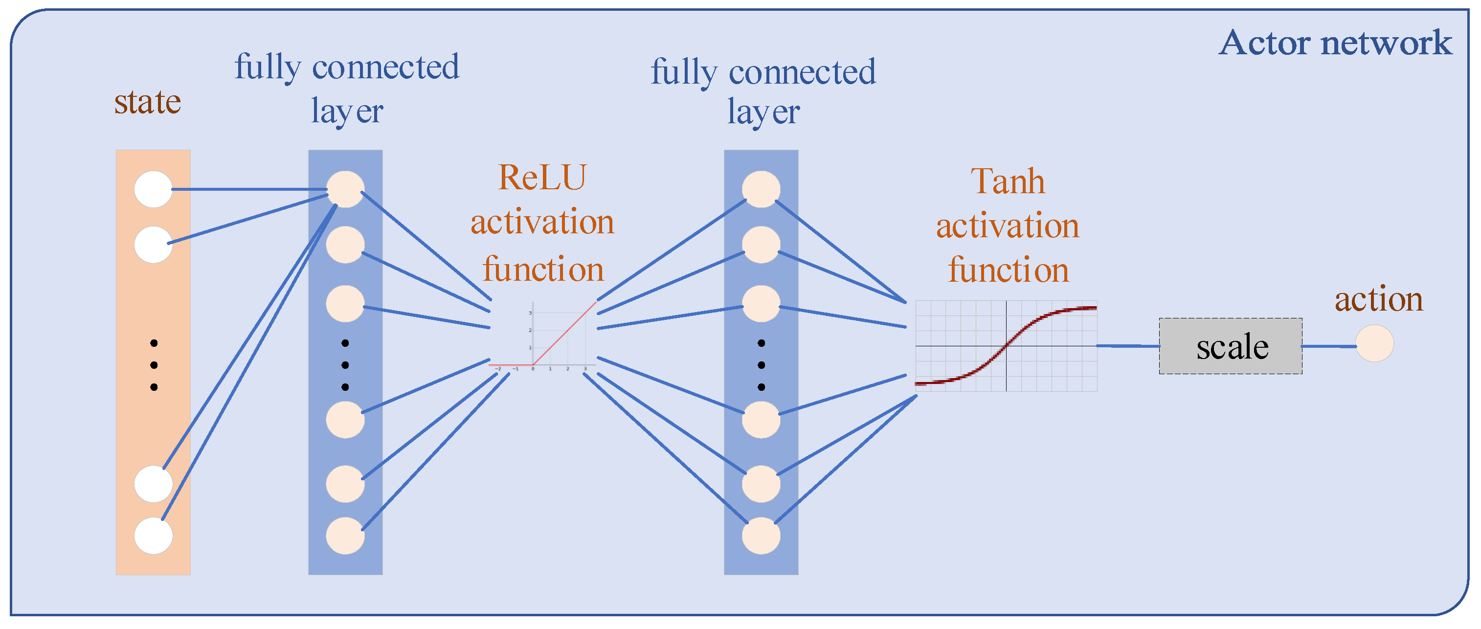
$\vartheta$ is the parameters of the policy network. Such a structure is called actor–critic. The Q network is used to export the action value, which is called the critic. The policy network output represents actions, which is called the actor. Specifically, the network structures used in this paper are shown in Figure 4 and Figure 5. Compared with the actor network, the critic network has a more complex structure. This difference enables the critic to infer the underlying state from the measurements and deal with the state transition.

In order to reduce the correlation of data and difficulty of training, this paper adopts the method of experiential replay and independent target network training. The algorithm flow presented in this paper is shown in Algorithm 1.

Algorithm 1 Attack and defense adversarial algorithm.

Randomly initialize Q network $q_w$ and policy network $g_{\vartheta }$ parameters  Initialize the target network parameters $q_w^t$ and $g_{\vartheta }^t$  Initialize the experience pool for $episode=1,2\cdots N$ do    Random initialization of penetration position, target area, static obstacle area and interceptor position within a certain range    for $i=1,2\cdots T$ do      State $S_1$ is obtained according to the local field of vision      Select the action based on the current state and exploration noise $a_t=g_{\vartheta }\left(S_t\right)+{\xi }_i$      Perform the action $a_t$,observe the return $r_t$, get the next state $s_{t+1}$      Put the sample $(s_t,a_t,r_t,s_{t+1})$ in the experience pool D      Sample random mini-batch of $(s_t,a_t,r_t,s_{t+1})$ from D      Optimize Critic network parameters w:      $Loss=MSE[q_w(s,a),r+\gamma q_{\overline{w}}](s^{\prime },a^{\prime })$      Optimize Actor network parameters $\theta$:      $Loss=-q_w(s,a)$      Every C steps update $\overline{w},\overline{\theta }$:      $\overline{w}=\tau w+(1-\tau )\overline{w}$,$\overline{\theta }=\tau \theta +(1-\tau )\overline{\theta }$    end for end for

The state input of DDPG is an 18-dimensional vector. They are 12-dimensional detection states, position $x_p,y_p$, speed $v_{xp},v_{yp}$ and position of the target area $(x_t,y_t)$, respectively. The action output is a 1-dimensional variable, i.e., the angular velocity of the penetrator.

3.1.1. Design of the Reward Function

In the confrontation scenario shown in Figure 1, the main objective of the penetrator is to break through the interception, bypass fixed obstacles, and reach the target area as soon as possible. At the same time, the movement range of the penetrator is limited. When it is intercepted, moves out of the boundary or hits static obstacles, the task fails, and this round of training is terminated in advance. The reward function is a key element in DRL that supervises agents to learn and obtain the optimal policy. The reward function consists of three parts:

$$\begin{array}{c}\hfill R_1={\beta }_1{R}_T+{\beta }_2{R}_P+{\beta }_3{R}_S,\end{array}$$

(2)

where $R_T$ is the instant reward associated with the distance between the target area, $R_P$ is the sparse penalty for terminating the round of training in advance, and $R_S$ is the instant reward associated with survival time. Specially, their expressions are as follows:

$$\begin{array}{c}\hfill R_T=\left\{\begin{array}{cc}20-D\hfill & D\le 1\hfill \\ 10-D\hfill & 1<D\le 2\hfill \\ 5-D\hfill & 2<D\le 3\hfill \\ 3-D\hfill & 3<D\le 4\hfill \\ -D\hfill & 4<D\hfill \end{array}\right.,\end{array}$$

(3)

where $D=\parallel X_P-X_t{\parallel }_2$.

$$\begin{array}{c}\hfill \left\{\begin{array}{cc}{R}_p=-800\hfill & ifterminateinadvance\hfill \\ R_S=20\hfill & ifsurvive\hfill \end{array}\right.\end{array}$$

(4)

Instant rewards can be obtained by the reward function at each time step. Therefore, the model can learn the specified functions on the condition that the reward function is designed reasonably. In this paper, ${\beta }_i(i=1,2,3)$ represents the weights of each reward function. Different weights cause different training results. When ${\beta }_3>0$, the agent is positively rewarded for survival and tends to learn to survive. However, when ${\beta }_3<0$, the agent is penalized for survival and tends to end the training as soon as possible. When a set of parameters is selected, the reward function is drawn as follows. It can be seen from Figure 6 and Figure 7 that the reward function is correctly set up to guide the agent toward the target area.

3.1.2. Reward Compensation and Incremental Training

In Equation (3), the reward function $R_T$ is related to the distance from the starting point to the target region, which causes the reward function to vary greatly with the initial points. The different sizes of the return functions make training harder. To solve this, a compensation reward is proposed:

$$\begin{array}{c}\hfill R_2={\int }_l{\parallel X_P-X_t\parallel }_{2}ds,\end{array}$$

(5)

where l is the directed line from $X_P$ to $X_t$.

In summary, the total reward function is

$$\begin{array}{c}\hfill R=\left\{\begin{array}{cc}{R}_1+R_2\hfill & ifsuccess\hfill \\ R_1\hfill & else\hfill \end{array}\right.\end{array}$$

(6)

It should be pointed out that incremental training scheme can effectively improve the training efficiency and reduce training times [13]. Therefore, the task is decomposed according to the difficulty of the training. Meanwhile, it should be noted that the weight of the reward functions should be adjusted reasonably in different training stages.

• In the early stage of training, the interceptor is not included. The main purpose is to train the agent to survive, and avoid the agent collision boundary and static obstacles;
• In the middle stage, the interceptor is also not included, but ${\beta }_3$ is decreased to make the agent reach the target area as soon as possible and avoid collisions;
• In the final stage, the interceptor is included. The further training enables the agent to break through the intercept.

3.1.3. Artificial Potential Field (APF) Based Path Planning Algorithm

APF is a widely used path planning algorithm at present [22]. Its basic principle is to construct an APF environment in which the target point provides gravity and the obstacles provide repulsion. The improved APF method is defined as

$$\begin{array}{c}\hfill \left\{\begin{array}{c}{U}_{atx}\left(x\right)=1/2k{(x-x_t)}^2\hfill \\ U_{aty}\left(y\right)=1/2k{(y-y_t)}^2\hfill \end{array}\right.,\end{array}$$

(7)

where k represents the gravitational gain, and $U_{at}(x,y)$ is the potential energy at $(x,y)$. The gravitation functions are expressed as

$$\begin{array}{c}\hfill \left\{\begin{array}{c}{F}_{atx}\left(x\right)=-grad[U_{atx}\left(x\right)=-k(x-x_t)]\hfill \\ F_{aty}\left(y\right)=-grad[U_{aty}\left(y\right)=-k(y-y_t)]\hfill \end{array}\right.\end{array}$$

(8)

The repulsive potential field function generated by the obstacles is defined as

$$\begin{array}{c}\hfill U_{re}(x,y)=\left\{\begin{array}{cc}1/2\eta {[1/\rho -1/{\rho }_0]}^2{d}^2\hfill & \rho \le {\rho }_0\hfill \\ 0\hfill & \rho >{\rho }_0\hfill \end{array}\right.\end{array}$$

(9)

$$\begin{array}{c}\hfill d=\sqrt{{(x-x_t)}^2+{(y-y_t)}^2}\end{array}$$

(10)

$$\begin{array}{c}\hfill \rho =\sqrt{{(x-x_b)}^2+{(y-y_b)}^2}-r,\end{array}$$

(11)

where $\eta$ is the repulsive gain coefficient, $\rho$ represents the shortest distance between the agent and the obstacles, and r is the radius of the obstacles. ${\rho }_0$ is a constant parameter, represents the influence range of the obstacles. Similarly, the repulsion functions are expressed as

$$\begin{array}{c}\hfill F_{rex}=\left\{\begin{array}{cc}{F}_{rex1}+F_{rex2}\hfill & \rho \le {\rho }_0\hfill \\ 0\hfill & \rho >{\rho }_0\hfill \end{array}\right.\end{array}$$

(12)

$$\begin{array}{c}\hfill F_{rey}=\left\{\begin{array}{cc}{F}_{rey1}+F_{rey2}\hfill & \rho \le {\rho }_0\hfill \\ 0\hfill & \rho >{\rho }_0\hfill \end{array}\right.,\end{array}$$

(13)

where

$$\begin{array}{c}\hfill \left\{\begin{array}{c}{F}_{rex1}=\eta [\frac{1}{\rho }-\frac{1}{{\rho }_0}]\frac{1}{{\rho }^3}(x-x_b)d^2\hfill \\ F_{rey1}=\eta [\frac{1}{\rho }-\frac{1}{{\rho }_0}]\frac{1}{{\rho }^3}(y-y_b)d^2\hfill \end{array}\right.\end{array}$$

(14)

$$\begin{array}{c}\hfill \left\{\begin{array}{c}{F}_{rex2}=-\eta {[\frac{1}{\rho }-\frac{1}{{\rho }_0}]}^2(x-x_t)\hfill \\ F_{rey2}=-\eta {[\frac{1}{\rho }-\frac{1}{{\rho }_0}]}^2(y-y_t)\hfill \end{array}\right.\end{array}$$

(15)

3.1.4. Proportional Guidance-Based Interception Algorithm

The proportional guidance is to make the interceptor’s rotational angular velocity proportional to the line-of-sight angular velocity. Assuming that the position of the interceptor is $x_b,y_b$, the speed is $v_{xb},v_{yb}$, the position of the penetrator is $x,y$, and the speed is $v_x,v_y$. The relative position and speed of the interceptor to the penetrator are shown in (16):

$$\begin{array}{c}\hfill \left\{\begin{array}{c}{x}_r=x_b-x\hfill \\ y_r=y_b-y\hfill \\ v_{xr}=v_{xb}-v_x\hfill \\ v_{yr}=v_{yb}-v_y\hfill \end{array}\right.\end{array}$$

(16)

The interceptor’s line-of-sight angle to the penetrator can be obtained as

$$\begin{array}{c}\hfill q=arctan\left(\frac{x_r}{y_r}\right)\end{array}$$

(17)

and the angle’s rate can be written as

$$\begin{array}{c}\hfill \dot{q}=\frac{v_{yr}{x}_r-v_{xr}{y}_r}{x_r^2+y_r^2}\end{array}$$

(18)

Then, the angular velocity of the interceptor can be obtained by

$$\begin{array}{c}\hfill {\omega }_b=K\left(\dot{q}\right),\end{array}$$

(19)

where K is the coefficient. In this paper, $K=2$ and $K=3$, respectively.

4. Simulations and Results

4.1. Simulations Based on RL

The parameters are shown in

Table 1. Parameters of the scenario.

Item	Value
Boundaries (m)	$-1\le x\le 20,-1\le y\le 20$
Speed of the penetrator (m/s)	$v_p=1$
Angular velocity of the penetrator (rad/s)	$-0.5\le {\omega }_p\le 0.5$
Speed of interceptors (m/s)	$v_b=1.2$
Angular velocity of interceptors (rad/s)	$-0.4\le {\omega }_b\le 0.4$
Radius of obstacles (m)	$r=0.7$
Radius of the target area (m)	$r_t=1$
Intercept radius (m)	$r_b=0.3$
Detection radius of the penetrator (m)	$r_p=1$
The target area (m)	$10\le x_t\le 12,10\le y_t\le 12$
Initial area of the penetrator (m)	$0\le x\le 1,0\le y\le 1$
Initial direction of the penetrator (rad/s)	$\pi /4$
Initial position of interceptors	$(x_t,y_t,\pi /4rad)$

.

The three subtasks all adopt the same network structure, as Figure 4 and Figure 5 show. The weight factors ${\beta }_1,{\beta }_2,{\beta }_3$ are changed only during the training. Figure 8 shows the training results for different subtasks.

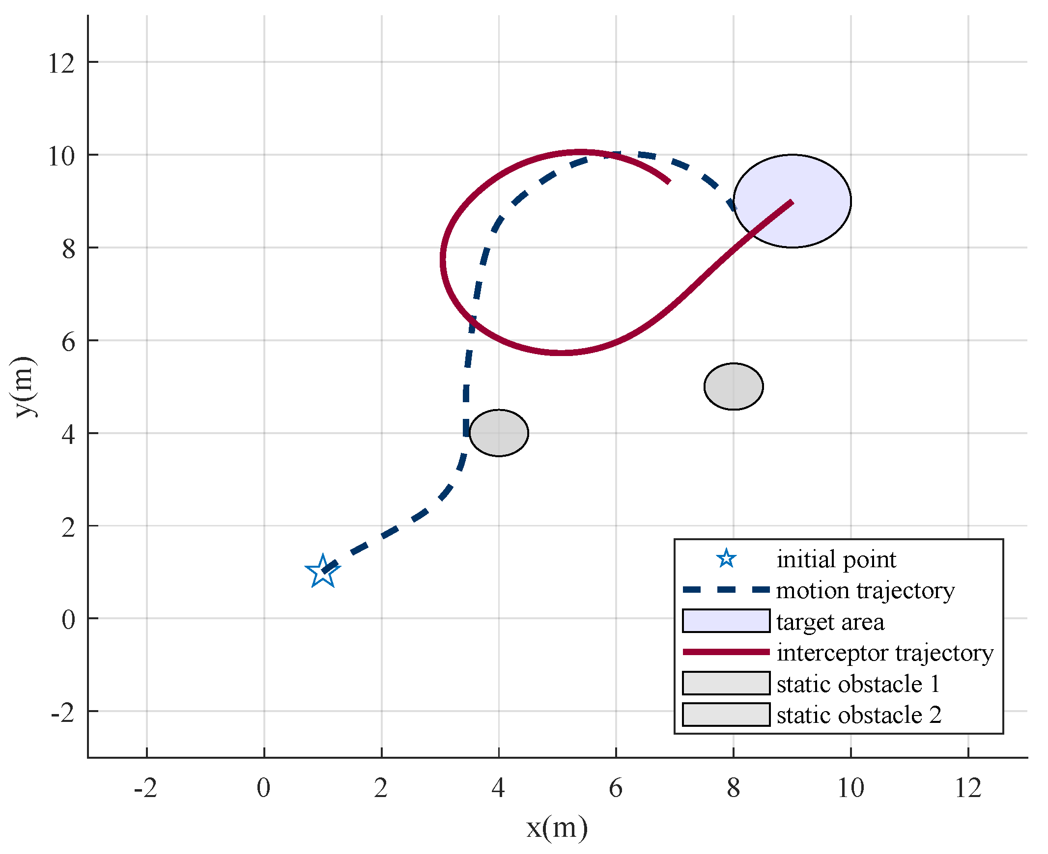
Figure 8a shows that the agent adopts a random strategy and exceeds the boundary before training. After the first and the second stages of training, the penetrator finds the shortest path that meets its overload constraint to reach the target area. However, when the proportional guidance-based interceptors are added, the penetrator is blocked, as Figure 8c illustrates. After further training, the agent learns to penetrate finally, as Figure 8d shows.

In the scene shown in Figure 8d, the angular velocity of the penetrator and the interceptor is illustrated in Figure 9. It can be seen that the penetrator reaches its maximum overload for penetration. Figure 10 illustrates the line-of-sight angles and their rates. The line-of-sight angles change rapidly with the decrease in the relative distance. This increases the difficulty of interception and is conducive to the penetration. The penetrator breaks through the interception by taking advantage of its higher maneuverability, which proves the effectiveness of the penetration strategy.

4.2. Simulations of Contrast Algorithm

To compare the effectiveness of the proposed algorithm, the APF-based path planning algorithm is adopted. Figure 11 and Figure 12 show that APF is usable when facing static obstacles. However, when the interceptor is added, APF is no longer valid, or the parameters need to be tuned carefully. Figure 13 and Figure 14 show that the penetrator is intercepted for its slow-change line-of-sight angle. However, the RL approach enables the intuitive setting of performance objectives, shifting the focus toward what should be achieved, rather than how, which simplifies the design process [23].

Furthermore, when there is no reward compensation, Figure 15 illustrates that, although the network can still converge, the total rewards vary greatly based on the distances from the initial points to the target area. Even if the same policy is adopted, the total rewards obtained from different initial points are quite different, and it is difficult to effectively judge the convergence of the network, which increases the difficulty of training. On the other hand, when the initial point is closer to the target point, due to the high rewards, even if a suboptimal strategy is adopted, an acceptable reward can also be obtained, which makes it difficult to converge to the optimal strategy. When the reward function without compensation is used, agents only obtain the suboptimal strategy, and the selected route is not the optimal one. However, when the reward compensation is adopted, the total rewards are independent of the distances, which is more beneficial to train to find the shortest path, as shown in Figure 16.

4.3. Monte Carlo Experiments

To verify the stability and generalization of the algorithm, 100 Monte Carlo experiments were carried out. In all simulations, the initial point, target area, and obstacles were randomly initialized within a certain range. The results are shown in Figure 17 and Figure 18, with a high success rate of $84\%$. It can be seen from the simulations that, in similar scenarios, agents are able to choose the learned optimal policy. That is, DRL converged to the optimal strategy through training. The simulation results also indicate that the method proposed has the generalization ability to a certain extent.

Through the analysis of failure cases, it is found that 50% of the cases are caused by a limited field of vision and low maneuverability, but the others are caused by wrong decision making.

4.4. Simulation Results in the Webots Simulator

Unlike the mathematical model created in Matlab, which is simplified to a second-order system, robots are more complex in the physical world. Webots is an open-source and multi-platform desktop application used to simulate robots. It provides a complete development environment to model, program and simulate robots. Hence, the Webots simulator is employed to verify the reliability of the algorithm proposed.

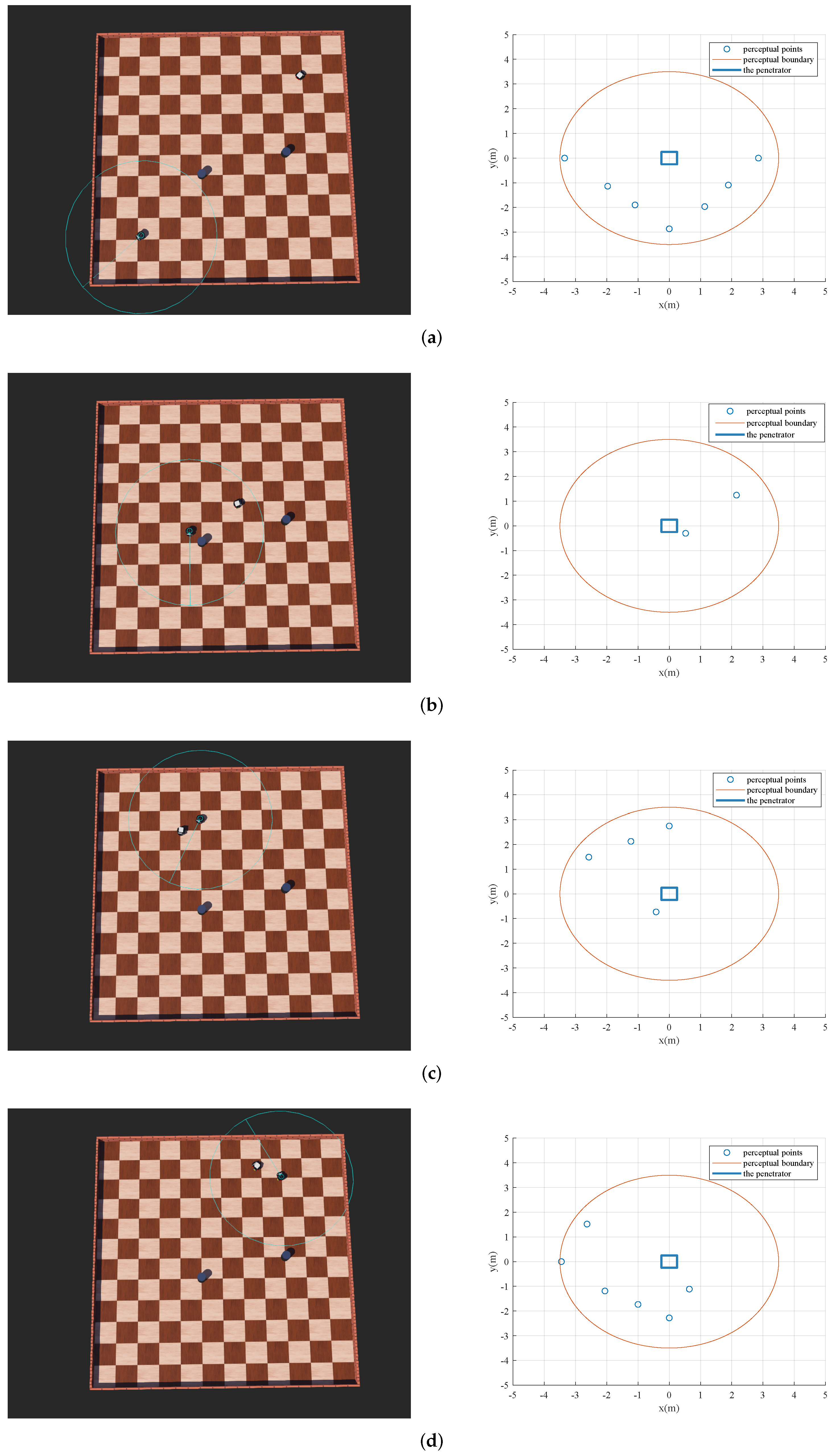
The environment and the robots are modeled as Figure A1a illustrates. In Webots, a one-layer LiDAR with a range of up to 3.5 m and a field of view up to 360 degrees is used to sense the surrounding environment. Its standard deviation of the Gaussian depth noise is 0.0043 m. At the same time, motor models are also added to simulate robots in the real world. The detection results in different stages are shown in Figure A1a–d, and the motion trails of the penetrator and the interceptor are shown in Figure 19.

It can be seen from the results above that the penetration algorithm proposed in this paper not only has a good performance in mathematical models, but also has feasibility in the Webots simulator.

5. Conclusions

In order to solve the problem that traditional methods-based robots cannot effectively break through the interception in a rejection environment, this paper proposes the DRL-based interception strategy. Aiming at addressing the issues of poor convergence of DRL, an incremental training method is proposed. The task is divided into three sub-tasks, and the agent is trained to gradually learn to survive, reach the target area, and break through the interception. Meanwhile, in order to reduce the difficulty of training and improve the training effect, reward compensation is adopted. The simulation results show that the introduction of reward compensation can unify the total return, which is beneficial for the agent to converge to the optimal policy. The simulation results in Webots also demonstrate the feasibility of the proposed algorithm in practical applications. In contrast, APF-based agents can only bypass static obstacles, but cannot break through the interception of interceptors. Navigation in the 3D environment is challenging, and we intend to refine this approach to make it applicable in our future work.

References

- Zhang, H.; Huang, C.; Zhang, Z.; Wang, X.; Han, B.; Wei, Z.; Li, Y.; Wang, L.; Zhu, W. The Trajectory Generation of UCAV Evading Missiles Based on Neural Networks. In Journal of Physics: Conference Series; IOP Publishing: Bristol, UK, 2020; Volume 1486, p. 022025. [Google Scholar]
- Yang, C.; Wu, J.; Liu, G.; Zhang, Y. Ballistic Missile Maneuver Penetration Based on Reinforcement Learning. In Proceedings of the 2018 IEEE CSAA Guidance, Navigation and Control Conference (CGNCC), Xiamen, China, 10–12 August 2018; pp. 1–5. [Google Scholar]
- Yan, T.; Cai, Y.; Bin, X. Evasion guidance algorithms for air-breathing hypersonic vehicles in three-player pursuit-evasion games. Chin. J. Aeronaut. 2020, 33, 3423–3436. [Google Scholar] [CrossRef]
- Nguyen, H.; La, H. Review of deep reinforcement learning for robot manipulation. In Proceedings of the 2019 Third IEEE International Conference on Robotic Computing (IRC), Naples, Italy, 25–27 February 2019; pp. 590–595. [Google Scholar]
- Li, Y. Deep reinforcement learning: An overview. arXiv 2017, arXiv:1701.07274. [Google Scholar]
- Buşoniu, L.; de Bruin, T.; Tolić, D.; Kober, J.; Palunko, I. Reinforcement learning for control: Performance, stability, and deep approximators. Annu. Rev. Control. 2018, 46, 8–28. [Google Scholar] [CrossRef]
- Dulac-Arnold, G.; Mankowitz, D.; Hester, T. Challenges of real-world reinforcement learning. arXiv 2019, arXiv:1904.12901. [Google Scholar]
- Lillicrap, T.P.; Hunt, J.J.; Pritzel, A.; Heess, N.; Erez, T.; Tassa, Y.; Silver, D.; Wierstra, D. Continuous control with deep reinforcement learning. arXiv 2015, arXiv:1509.02971. [Google Scholar]
- Zhang, C.; Song, W.; Cao, Z.; Zhang, J.; Tan, P.S.; Xu, C. Learning to dispatch for job shop scheduling via deep reinforcement learning. arXiv 2020, arXiv:2010.12367. [Google Scholar]
- Kober, J.; Bagnell, J.A.; Peters, J. Reinforcement learning in robotics: A survey. Int. J. Robot. Res. 2013, 32, 1238–1274. [Google Scholar] [CrossRef] [Green Version]
- Lei, X.; Zhang, Z.; Dong, P. Dynamic path planning of unknown environment based on deep reinforcement learning. J. Robot. 2018, 2018, 5781591. [Google Scholar] [CrossRef]
- Zhao, W.; Liu, H.; Lewis, F.L. Robust formation control for cooperative underactuated quadrotors via reinforcement learning. IEEE Trans. Neural Netw. Learn. Syst. 2020, 32, 4577–4587. [Google Scholar] [CrossRef] [PubMed]
- Gao, J.; Ye, W.; Guo, J.; Li, Z. Deep reinforcement learning for indoor mobile robot path planning. Sensors 2020, 20, 5493. [Google Scholar] [CrossRef] [PubMed]
- Choi, J.; Park, K.; Kim, M.; Seok, S. Deep reinforcement learning of navigation in a complex and crowded environment with a limited field of view. In Proceedings of the 2019 International Conference on Robotics and Automation (ICRA), Montreal, QC, Canada, 20–24 May 2019; pp. 5993–6000. [Google Scholar]
- Faust, A.; Oslund, K.; Ramirez, O.; Francis, A.; Tapia, L.; Fiser, M.; Davidson, J. Prm-rl: Long-range robotic navigation tasks by combining reinforcement learning and sampling-based planning. In Proceedings of the 2018 IEEE International Conference on Robotics and Automation (ICRA), Brisbane, Australia, 21–25 May 2018; pp. 5113–5120. [Google Scholar]
- Feng, S.; Sebastian, B.; Ben-Tzvi, P. A Collision Avoidance Method Based on Deep Reinforcement Learning. Robotics 2021, 10, 73. [Google Scholar] [CrossRef]
- Dai, P.; Yu, W.; Wen, G.; Baldi, S. Distributed reinforcement learning algorithm for dynamic economic dispatch with unknown generation cost functions. IEEE Trans. Ind. Inform. 2019, 16, 2258–2267. [Google Scholar] [CrossRef] [Green Version]
- Wang, B.; Liu, Z.; Li, Q.; Prorok, A. Mobile robot path planning in dynamic environments through globally guided reinforcement learning. IEEE Robot. Autom. Lett. 2020, 5, 6932–6939. [Google Scholar] [CrossRef]
- Busoniu, L.; Babuska, R.; De Schutter, B. A comprehensive survey of multiagent reinforcement learning. IEEE Trans. Syst. Man Cybern. Part C (Appl. Rev.) 2008, 38, 156–172. [Google Scholar] [CrossRef] [Green Version]
- De Witt, C.S.; Peng, B.; Kamienny, P.A.; Torr, P.H.; Böhmer, W.; Whiteson, S. Deep multi-agent reinforcement learning for decentralized continuous cooperative control. arXiv 2020, arXiv:2003.06709. [Google Scholar]
- Silver, D.; Lever, G.; Heess, N.; Degris, T.; Wierstra, D.; Riedmiller, M. Deterministic policy gradient algorithms. In Proceedings of the 31st International Conference on Machine Learning, Beijing, China, 21–26 June 2014; pp. 387–395. [Google Scholar]
- Kumar, P.B.; Rawat, H.; Parhi, D.R. Path planning of humanoids based on artificial potential field method in unknown environments. Expert Syst. 2019, 36, e12360. [Google Scholar] [CrossRef]
- Degrave, J.; Felici, F.; Buchli, J.; Neunert, M.; Tracey, B.; Carpanese, F.; Ewalds, T.; Hafner, R.; Abdolmaleki, A.; de Las Casas, D.; et al. Magnetic control of tokamak plasmas through deep reinforcement learning. Nature 2022, 602, 414–419. [Google Scholar] [CrossRef] [PubMed]
Figure 1.
The confrontation scenario.
Figure 2.
The sensory ability of the penetrator.
Figure 3.
The structure of DDPG.
Figure 4.
Structure of the actor network.
Figure 5.
Structure of the critic network.
Figure 6.
The reward function.
Figure 7.
Top view of reward function.
Figure 8.
Results in different training stages. (a) Out of bounds before training; (b) the shortest path to reach the target area; (c) intercepted by the interceptors; (d) break through the interception.
Figure 9.
Angle velocity of agents.
Figure 10.
Line-of-sight angles and their rate.
Figure 11.
Artificial field.
Figure 12.
Motion trail based on APF.
Figure 13.
Motion trail with interceptor based on APF.
Figure 14.
Line-of-sight angle and its rate based on APF.
Figure 15.
Total rewards with and without compensation.
Figure 16.
Motion trails with and without compensation.
Figure 17.
Trajectories in the Monte Carlo experiments.
Figure 18.
The 100 Monte Carlo experiments.
Figure 19.
Simulation results in Webots.