1. Introduction
Parallel robots are mechanical structures different from a traditional serial manipulator, which generally consists of multiple closed motion loops. Reymond developed the parallel prototype of the manipulator in 1988, which is called the Delta robot [
1]. The Delta Robot is a three-degrees-of-freedom space mechanism with three revolute legs, i.e., each leg is connected to the fixed platform and the moving platform by a set of spherical joints. Moreover, the motion of the Delta robot is controlled by three motors that are mounted on the base. The three motors actuate the three legs to realize the movement of the moving platform.
Dynamics modeling of the parallel robotic manipulators is important for the machine’s motion control [
2,
3,
4,
5] and its corresponding structure design [
6,
7]. Many researchers have studied the dynamics modeling methods of parallel manipulators. The following are the main methods:
- (1)
The Newton–Euler method establishes the dynamics model of the parallel manipulator. This method was applied by Kourosh E. Zanganeh to a six-degree-of-freedom parallel robot [
8]. The parallel robot consists of six legs connected to a moving platform and a fixed platform. Each leg passes through a universal joint and a spherical joint to form two revolving joints; Chunxia Zhu used Newton’s second law to derive the dynamics model of a 3-TPT flexible parallel robot [
9]; Swain proposed a general dynamics model derivation method for manipulators [
10]; George H. Pfreundschuha proposed a dynamics model for a pneumatic parallel robot with three degrees of freedom [
11].
- (2)
The Lagrangian method establishes the dynamics model of the parallel manipulator. G. Lebret usedthe Lagrangian method to analyze the dynamics of the Stewart parallel platform [
12].
- (3)
Kane’s method establishes the dynamics model of a parallel manipulator. This method is proposed by Kane [
13]. Liu used the Huston form of Kane’s equation to derive the positive dynamics equation of the Gough–Stewart manipulator [
14].
- (4)
The virtual work principle establishes the dynamics model of a parallel manipulator. Tsai used the virtual work principle and the Jacobian matrix to derive the inverse dynamics model of the Gough–Stewart manipulator [
15]. F. Caccavale proposed a dynamics modeling of Tricept robot. Its parallel structure has three DOFs which are described by the axial translation of the radial link, and by two rotations about two axes orthogonal to the link itself [
16].
In this paper, the object of study is a parallel robot with four degrees of freedom, which is based on the structure of the Delta robot [
17,
18,
19]. With reference to
Figure 1, a telescopic rod connecting the fixed platform and the moving platform allows the flange on the moving platform to rotate around the
Z-axis.
In recent years, extensive research has been reported on dynamics analysis of the Delta robot [
20,
21,
22,
23]. However, these works focus on the traditional Delta robot and do not consider the effect of the telescopic rod on the actuator torques. In this paper, we use the Lagrangian method to establish a dynamics model of the telescopic rod. Moreover, these equations are implemented in an algorithm that is used to study the telescopic rod influence on actuator torques. The application of this algorithm is illustrated through a numerical example that simulates the dynamic behavior of the telescopic rod and actuators while following a sample trajectory.
2. Kinematics
Manipulator kinematics studies the movement of connecting rods under geometric constraints. In general, manipulator kinematics includes two parts: forward kinematics and inverse kinematics. The purpose of the forward kinematics solution is to determine the position of the moving platform using the input of the actuators. The purpose of the inverse kinematics solution is to determine the input of the actuators by determining the position of the moving platform.
Because this paper aims to build a complete dynamics model of the Delta robot with a telescopic rod, it is necessary to study the relationship between the motion of the telescopic rod and position of the moving platform. Therefore, we divide the kinematics into two parts. The first part is the Delta robot kinematics, and the second part is to obtain the telescopic rod kinematics under the condition that the telescopic rod is regarded as a subsystem. The telescopic rod kinematics model and Jacobian matrix are proposed, and are used to study the relationships among the movement of the telescopic rod, the movement of the moving platform, and the actuator torques.
2.1. Robot Structure
The structure diagram of the Delta robot with a telescopic rod is shown in
Figure 2, where numbers 1 and 2 represent the fixed platform and the moving platform, respectively. Three identical mechanical arms are connected to the fixed platform and the moving platform. Each mechanical arm consists of an upper arm and a lower arm. The upper arms are labeled 3, 4 and 5, and the lower arms are labeled 6, 7 and 8. The upper arm is connected to the drive motor to form rotating joints of
,
and
. The upper arms and the lower arms are connected by ball hinge joints of
,
and
. The lower arms have a parallelogram structure and are connected with the moving platform through ball hinge joints of
,
and
. The telescopic rod is labeled 9, and is directly connected to the moving platform and the fixed platform, which realizes the rotation of the end effector.
The coordinate system XYZ is attached to the center of the fixed platform at point O. The X-axis and Y-axis lie in the same plane as defined by the joints of , and . defines the angular orientation of the leg relative to the XYZ frame on the fixed platform.
2.2. Forward Kinematics
The purpose of studying forward kinematics is to be able to obtain the position of the end effector through a given rotation angle. For this type of robot, the rotation angle of the upper arm is known. The position of the center of the moving platform in the XYZ coordinate system is derived by the rotation angle. Moreover, the movement of the telescopic rod can obtain the position of the movable platform by establishing the generalized coordinate system of the telescopic rod.
2.2.1. The Forward Kinematics of the Delta Robot without a Telescopic Rod
Because the movement of the moving platform in the XYZ coordinate system is determined by three legs with the same structure, a single leg i is used as the research object, and its structure is shown in
Figure 3.
With reference to
Figure 3, a coordinate system
is established at the joint
for each leg, such that the
-axis is perpendicular to the axis of rotation of the joint
. The
-axis is along the joint axis
. The angle
is measured from
to
. The angle
is defined from
to
. The angle
is measured from
to
. The length from the center of the fixed platform to the joint is
R, and the length from the center of the moving platform to the joint is
r. The lengths of the upper arms and the lower arms are denoted as
and
, respectively.
We can obtain the equation as follows:
where
,
and
are defined as:
The positions x, y and z of the center of the moving platform at angles , , are solved by Equation (1).
2.2.2. The Forward Kinematics of the Telescopic Rod System
The movement of the telescopic rod does not affect the position of the moving platform, but it will exert a force on the moving platform, which will affect the actuator torques. The kinematics of the telescopic rod is the basis for studying the influence of the telescopic rod motion on the actuator torques.
The telescopic rod is regarded as a subsystem of the robot whose base is a fixed platform and whose end is a moving platform. The base and the telescopic rod are connected by ball joints. The Grubler formula is used to analyze the degrees of freedom of the telescopic rod:
The n is rigid body degrees of freedom. N represents the number of mechanical components. K is the number of joints and is the degree of freedom of the Kth joint. For the telescopic rod, n = 3, N = 1, K = 1. The ball joint has three degrees of freedom, so the telescopic rod system has three degrees of freedom.
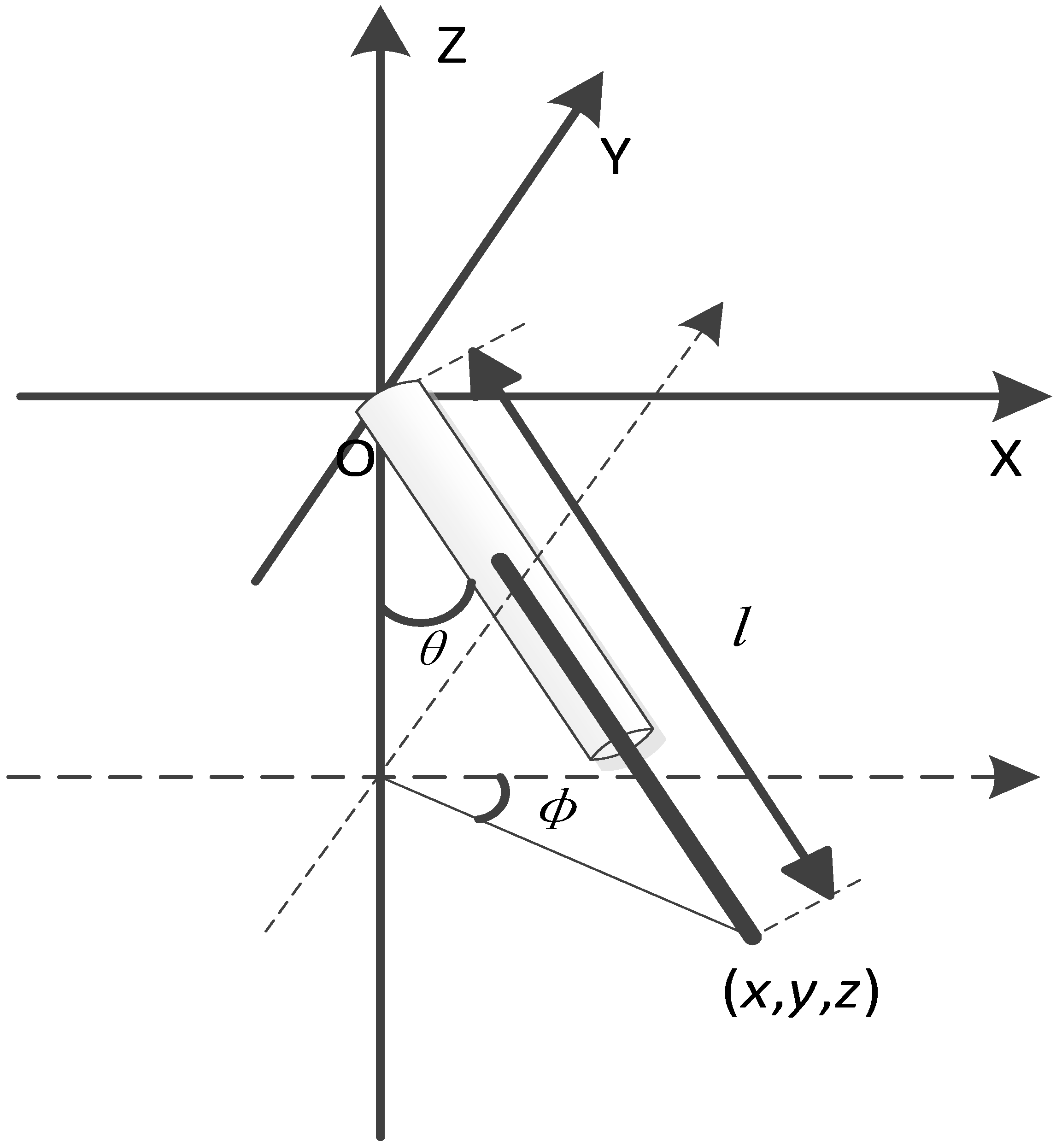
(1) The model of the telescopic rod is simplified, which is shown in
Figure 4. The
l is the length of the telescopic rod.
is the angle between the telescopic rod and the negative direction of the
z-axis.
is the angle between the projection of the telescopic rod on the XY plane and the positive direction of the
x-axis.
l,
and
are used as variables to describe the motion of the telescopic rod.
Defining
l,
,and
as the axis variable. The axis variables and the position of the moving platform have the following relationship:
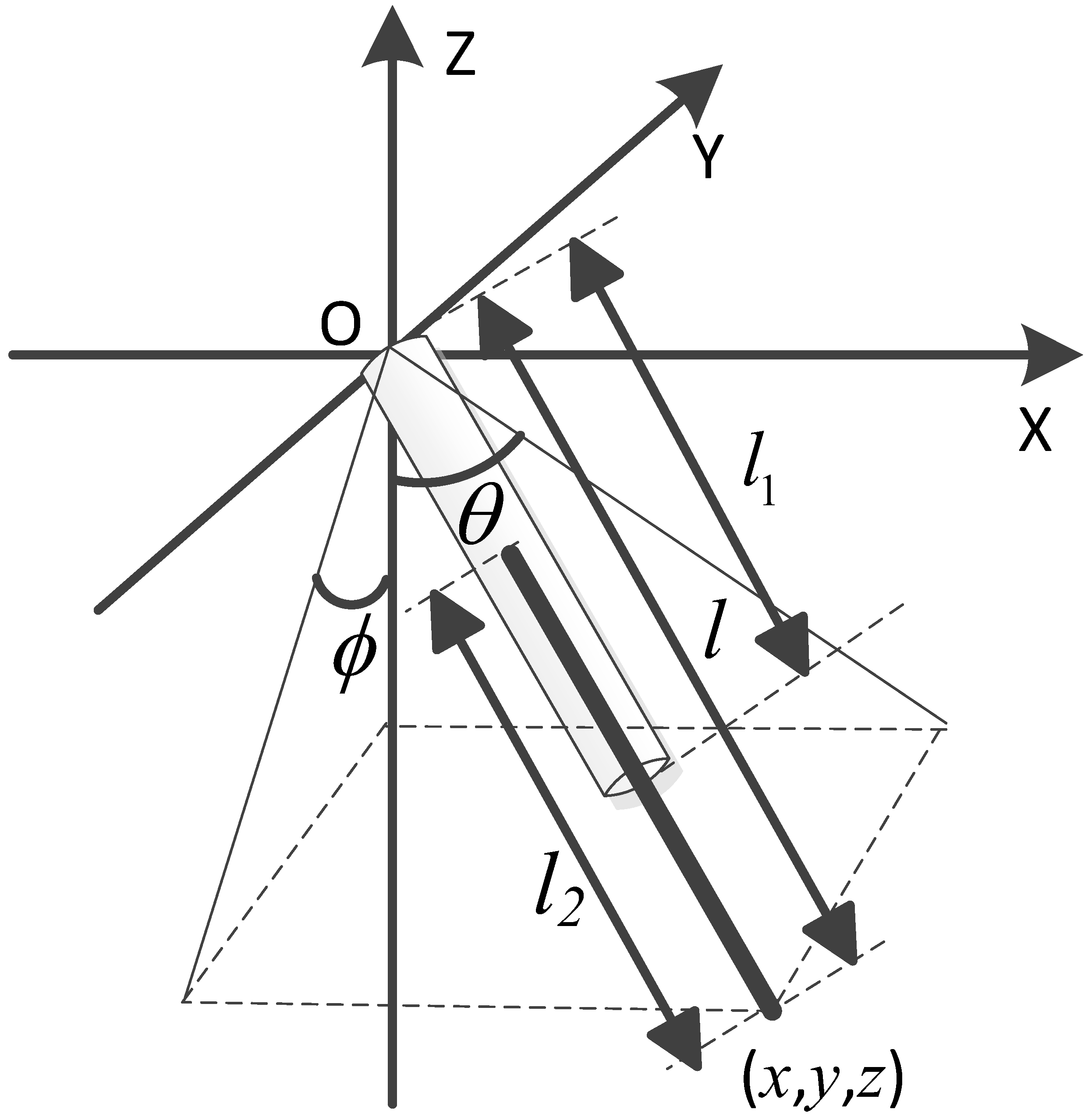
(2) Generalized coordinate system 2 is shown in
Figure 5.
l is the length of the telescopic rod.
is the angle between the projection of the rod in the XZ plane and the negative direction of the
z-axis.
is the angle between the projection of the rod in the YZ plane and the negative direction of the
Z-axis.
Similarly to generalized coordinate system 1, the axis variables and the position of moving platform have the following relationship:
We can obtain the forward kinematics of the telescopic rod from Equation (4):
2.3. Inverse Kinematics
A. The inverse kinematics of the Delta robot
The first part of inverse kinematics is to solve the angle of the upper arm given the target position. By analyzing the structure of the leg i, we can readily derive the expression below [
24]:
,
and
represent the position of
P in the
coordinate frame. The expressions for these variables are given by:
Therefore,
can be obtained by Equation (8):
We can obtain Equation (11) by summing the square of formula (7) and formula (9):
Moreover, using Equation (11), we can write:
where:
A. Half-angle tangent is defined as:
where
can be obtained by solving a polynomial Equation (12). Then,
can be solved using Equation (14):
B. The inverse kinematics of the telescopic rod system
The second part of the inverse kinematics solution is to obtain the description of the motion of the telescopic rod in the generalized coordinate system through the position of the moving platform.
The inverse kinematics in generalized coordinate system 1 is given as:
The inverse kinematics in generalized coordinate system 2 is given as:
2.4. Jacobian
A. The Jacobian of the Delta robot
The first part of the Jacobian matrix provides a transformation from the velocity of the end-effector in Cartesian space to the actuated joint velocities, as shown in Equation (17):
where
=
is the speed vector of the moving platform, and
=
is the rotation speed vector of the upper arms.
The Jacobian matrix of this part is defined as
where:
B. The Jacobian of the telescopic rod system
Differentiating both sides of Equation (2) with respect to time, we obtain:
Equation (20) can be derived by converting Equation (19) into matrix form:
where:
Similarly, differentiating both sides of Equation (5) with respect to time, we obtain:
where:
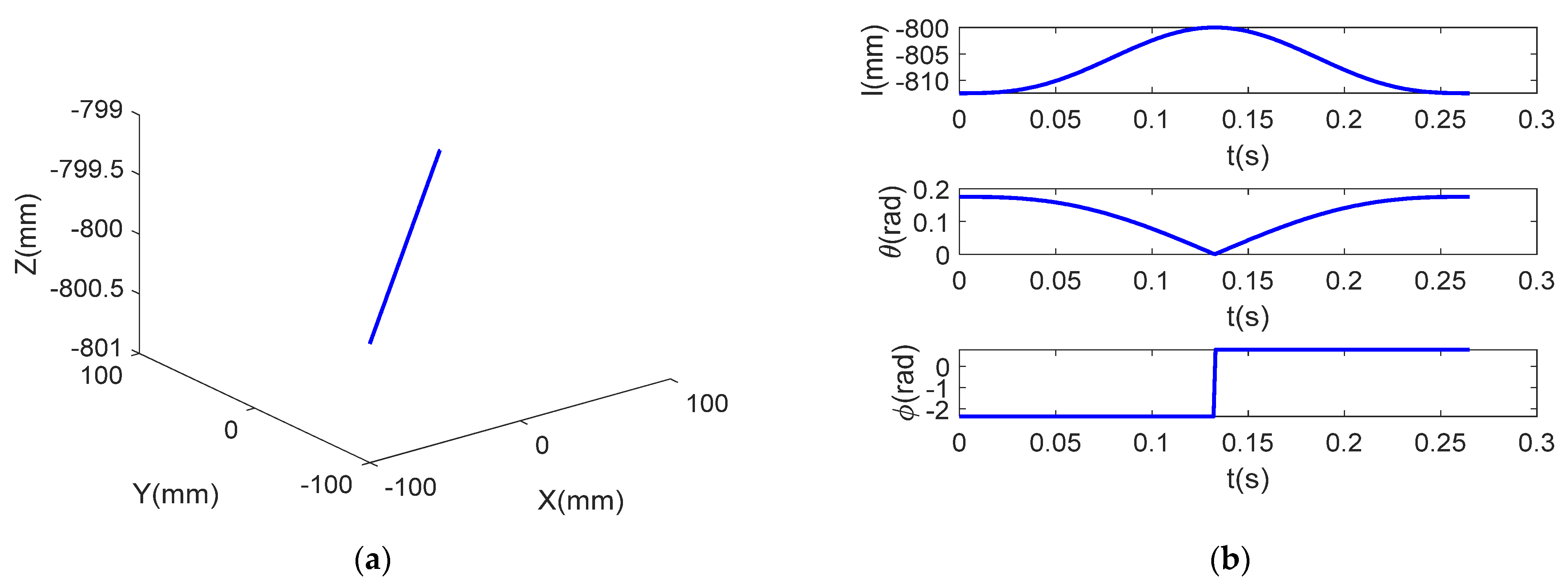
The kinematics and Jacobian matrices of telescopic rods in two generalized coordinate systems are established, respectively. In order to determine the kinematics of the telescopic rod in that generalized coordinate system, a singularity analysis is carried out on it. The singularities occur when the following condition is satisfied:
The determinant of
is zero when
is equal to zero. At the same time, this also means that when the position of the moving platform passes (0, 0, z), the value
will change suddenly. We have generated a linear trajectory in the Cartesian space from point (100, −100, −800) to (100, 100, −800), which is shown in
Figure 6a. We can see from
Figure 6b that the value of
has a big mutation, which will cause the Jacobian matrix at this time to be ill-conditioned. However, the representation of the same trajectory in generalized coordinate system 2, which has no singularity, is shown in
Figure 6c.
Therefore, generalized coordinate system 2 is used to describe the motion of the telescopic rod, because the determinant of will not appear to be zero matrices.
The Jacobian matrix of the telescopic rod and the Jacobian matrix of the Delta robot without a telescopic rod are derived through kinematics. This is important for establishing the dynamic model with the telescopic rod.
3. Dynamics
The actuator torques of traditional Delta robot are mainly used to drive the upper arms, lower arms and moving platform. However, the Delta robot with a telescopic rod also needs to drive the telescopic rod, which means that the original dynamics model can no longer accurately represent the relationship between the motion of robot and the actuator torques.
The movement of the telescopic rod is produced by the moving platform, and the actuator torque of the moving platform is produced by the servo motor. The force of the telescopic rod acting on the moving platform and the force of the moving platform acting on the telescopic rod are a pair of interaction forces. The movement of the telescopic rod is analyzed to obtain the force on the moving platform, and then to obtain the torque for the three actuators.
3.1. Dynamics of Telescopic Rod
In the above section, the relationship between the axis variables and the position of the moving platform is derived. Further, the Euler–Lagrange method is used to establish the dynamics equation of the telescopic rod, which is used to describe the relationship between the motion of the telescopic rod and the torque applied by the moving platform to the telescopic rod.
The Lagrangian function of the telescopic rod can be expressed as:
where
and
represent the total kinetic energy and potential energy of the telescopic rod, respectively.
The Euler–Lagrange equation of the telescopic rod is expressed as follows:
The structure of the telescopic rod is simplified into two parts, which are divided into an upper rod and a lower rod. The moment of inertia of the upper rod is:
The moment of inertia of the lower rod is:
where
and
are the masses of the upper rod and lower rod, respectively.
The kinetic energy of the upper rod and lower rod can be given as:
Similarly, we can obtain the potential energy equation of the upper rod and lower rod as follows:
We can readily obtain the telescopic rod Lagrangian function and Lagrangian equation through Equations (23) and (24).
where
is damping ratio, and
Equation (29) denotes the relationship between the motion of the telescopic rod and the torque generated by the virtual axis. Then, using the Jacobian matrix of the telescopic rod, the torque generated by virtual axis can be converted to torque from the moving platform. Finally, the traditional Jacobian matrix of the Delta robot is used to obtain actuator torques of the three upper arms, thereby obtaining:
3.2. Dynamics Modeling of Delta Robot with Telescopic Rod
On the one hand, the driving torques generated by the actuators make the telescopic rod move; on the other hand, they make the moving platform move by driving the upper arms. In order to obtain the driving torque through the motion of the moving platform, a complete dynamics model of the four-DOF parallel robot needs to be established.
Newton–Euler equations of motion are used to determine the torques applied by actuators without a telescopic rod [
24,
25]. This dynamics model assumes that the mass of each lower rod is concentrated at the joints
. Based on these assumptions, the equation of motion is written by summing the moments about the actuated joint for the
ith leg:
where
is the sum of the moments applied at joint
;
is the mass moment of inertia of the upper rod and the lower rod;
is the
ith element of
, which is an array of the inertial loads at joint
due to the acceleration of the moving platform; and
is the viscous damping coefficient of the actuators. The expressions for
and
are given by Equations (36) and (37):
where
is the mass moment of inertia of the motor rotor, and
is the acceleration of the moving platform.
Taking into account the motor torques and the gravitational force,
can also be expressed as:
Then, we can obtain actuator torques using Equations (35) and (38).
Furthermore, the total moment of the three actuators is given as:
where
can be obtained using Equation (33).
4. Simulations
To clearly present the proposed method, a numerically computed example will be discussed in this section. A trajectory for the moving platform and a set of manipulator design parameters are assumed. The gate-shaped trajectory is selected to represent a typical motion that might be used during a practical application of the Delta robot.
The Delta robot design parameters that are used for the simulations are given as:
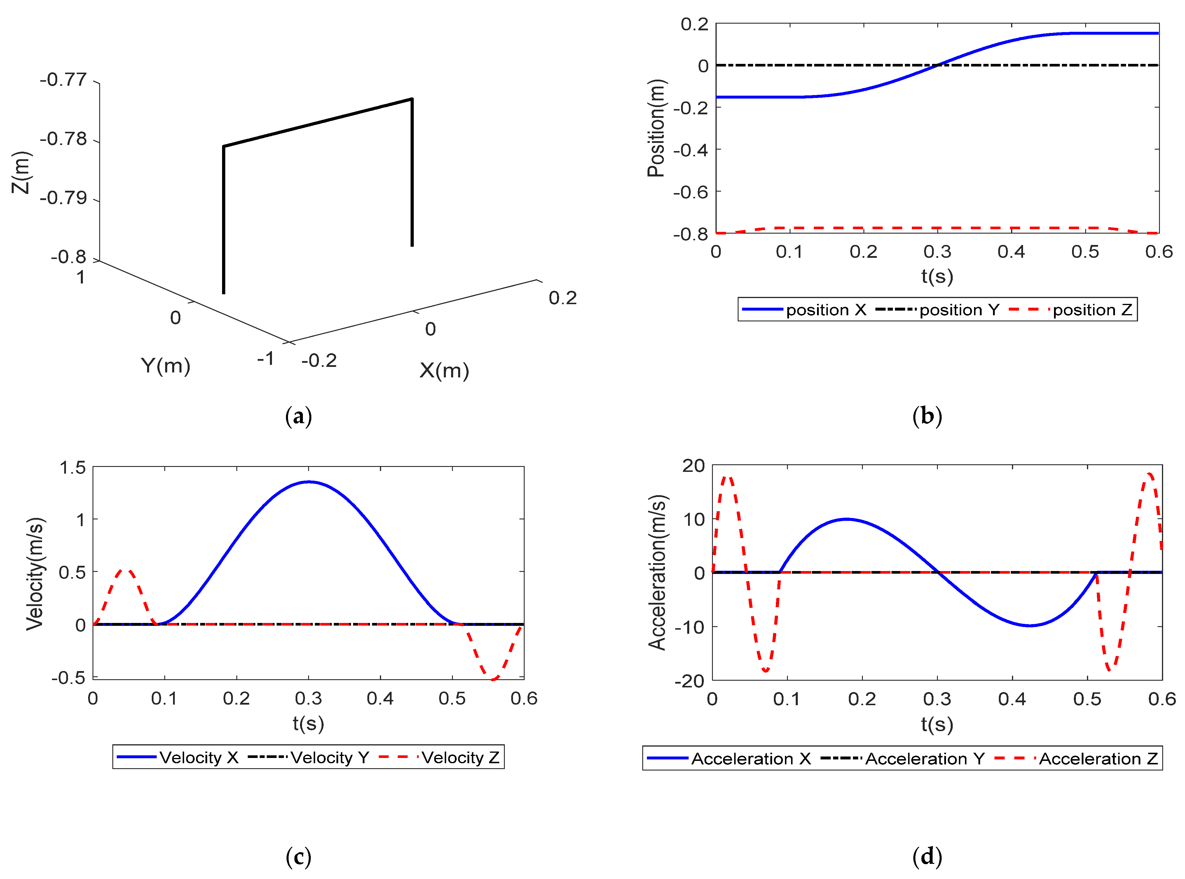
Firstly, taking a trajectory as the research object, its movement time is 0.6s and the damping ratio is zero. The trajectory is shown in
Figure 7a. The corresponding time-histories of the components of the position, velocity, and acceleration of the center of the moving platform are shown in
Figure 7b–d.
The axis variables of the telescopic rod can be obtained by the movement of the moving platform. The corresponding time-histories of the components of the position, velocity, and acceleration of the axis variables of the telescopic rod are shown in
Figure 8a–c. The moment of the telescopic rod on the moving platform is shown in
Figure 8d.
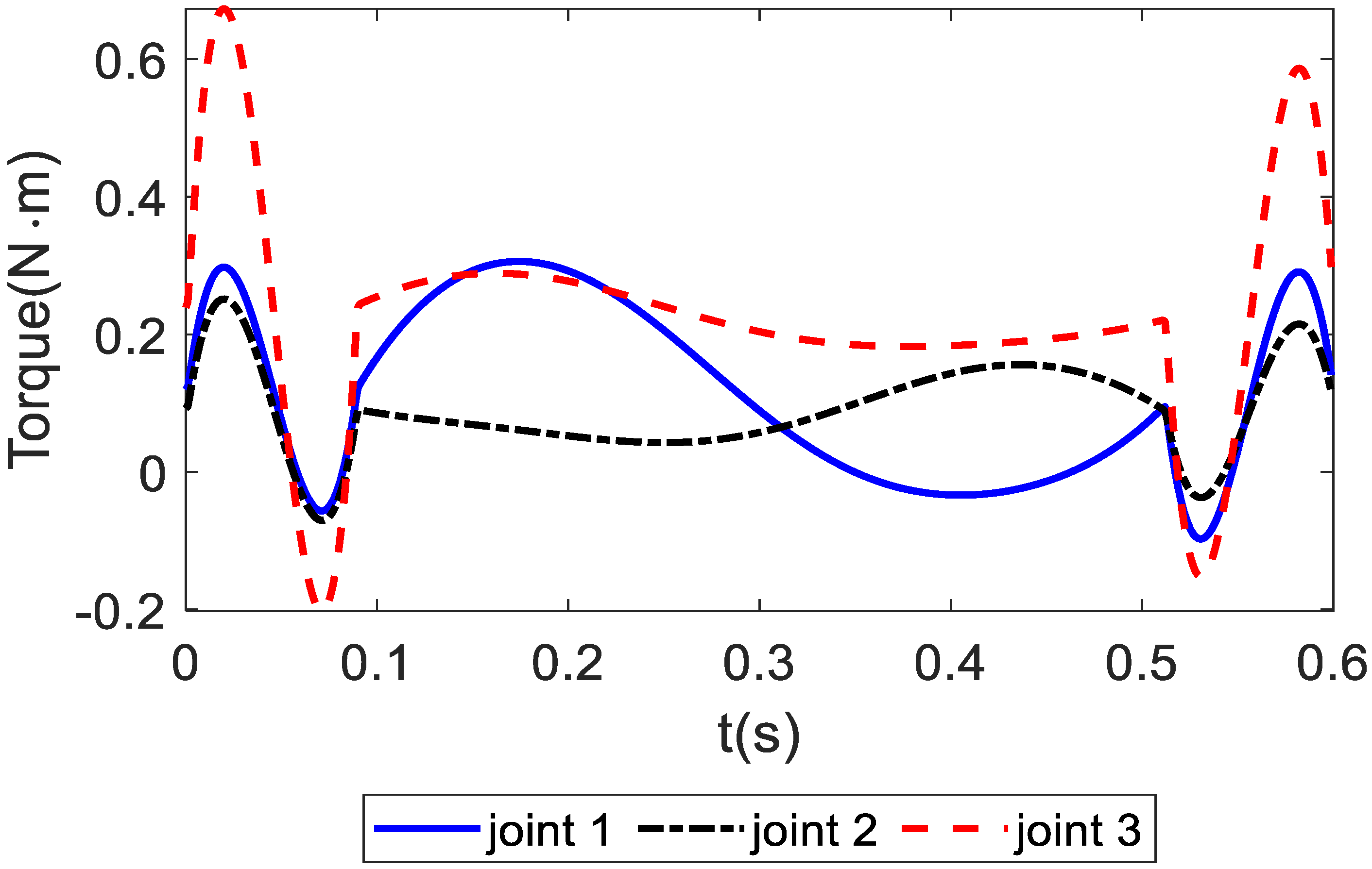
Given this sample trajectory and set of manipulator design parameters, the actuator torques of the Delta robot are calculated without the telescopic rod using the proposed approach. Next, using same trajectory and Delta robot design parameters, the actuator torques of the Delta robot with a telescopic rod are calculated. Friction is ignored when calculating the actuator torques. The results from these two simulations are shown in
Figure 9 and
Figure 10.
From the simulation results, it can be seen that the actuator torques with the telescopic rod and without the telescopic rod under the same trajectory are different, and the actuator torques with the telescopic rod are larger than those without the telescopic rod. This is because when there is a rod, the drive shaft not only drives the movement of the moving platform but also drives the movement of the telescopic rod.
5. Experimental Application
An experimental study is now presented to test the dynamics model of the Delta robot with a telescopic rod. First, the actuator torques with and without the telescopic rod are compared under the same trajectory, which is used to verify the effect of the telescopic rod on the actuator torques. Second, a robot control system based on the torque feedforward control strategy is built, and the effects of the traditional Delta robot dynamics model and the dynamics model proposed in this paper on trajectory tracking are compared.
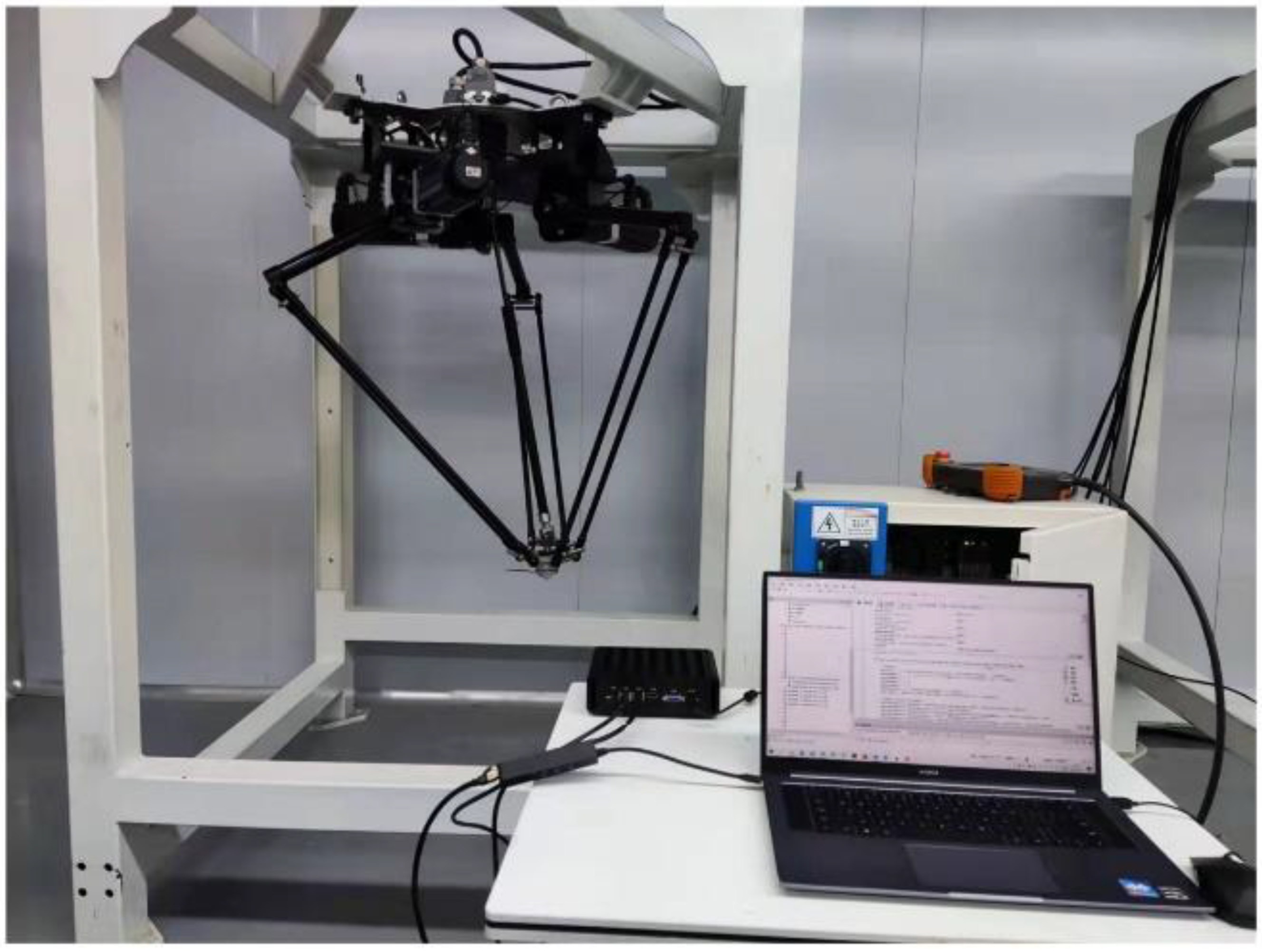
The experimental installation constitutes of a Delta robot with a telescopic rod, in which the original control unit has been replaced by an open control system developed by ourselves. The mechanical parameters can be seen in
Table 1. The experimental installation is shown in
Figure 11.
5.1. Comparing Actuator Torques
The above section discusses the effect of the telescopic rod motion on the actuator torques, and to verify this, an experiment is carried out. The robot is allowed move along a standard gate shape and collect the actuator torques. The actuator torques are collected again, along the same trajectory, without the telescopic rod.
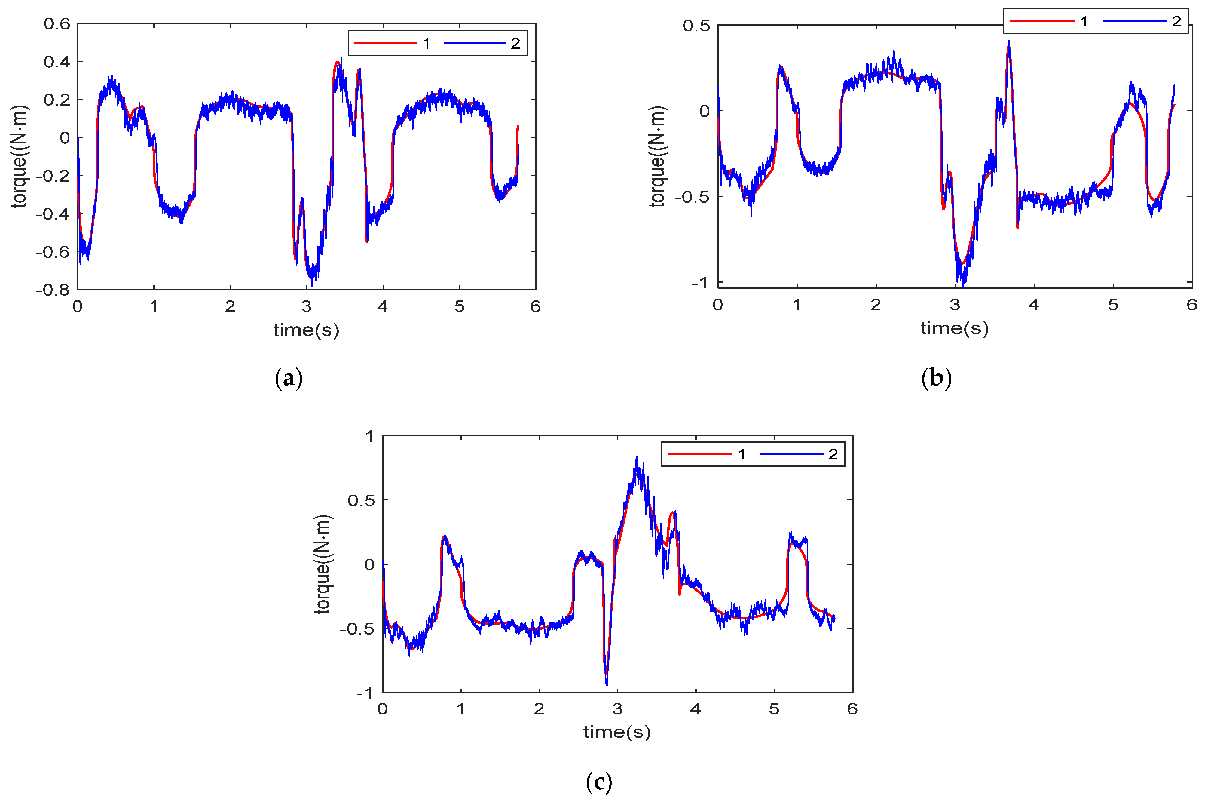
Two different sets of actuator torques, obtained from data measured from the Delta robot, are compared—the first one with a telescopic rod and the second one without a telescopic rod. A comparison between the actuator torques with telescopic rod and actuator torques without telescopic rod is shown in
Figure 12. It can be seen in the figure that the actuator torques are different in the two cases, and the actuator torques of the Delta robots with the telescopic rod are larger than those of the Delta robot without the telescopic rod when performing the same movement. The result indicates that the telescopic rod does have an effect on the actuator torques, and it is meaningful to study the effect of the torque produced by the telescopic rod.
5.2. Dynamics Parameter Identification
An important application of dynamics is to achieve more precise control, so the proposed dynamics are applied to torque feedforward control to compare the tracking errors with traditional robot dynamics. The torque feedforward control strategy needs to calculate the actuator torques in real-time according to the motion of the robot, which requires dynamics identification of the robot. The dynamics parameter identification of the Delta robot with a telescopic rod is divided into two parts. The first part is to identify the inertial parameters of the three legs. The second part is to identify the inertial parameters of the telescopic rod according to Equation (40).
The optimized trajectory used to perform the parameter identification is parameterized as a finite Fourier series according to the method described in Ref. [
26]. The identification algorithm can be divided into two steps:
(1) Dynamics parameter identification for Delta robot without telescopic rod
The friction force is a non-negligible item in the actuator torques, so the friction force is considered based on Equation (39). The actuator torques without the telescopic rod can be expressed as:
where
is the friction force, and can be described as a coulomb viscous friction model.
Linearizing Equation (41), we obtain:
where
I is the parameter to be identified. The identification parameters can be obtained using the least squares method.
(2) dynamics parameter identification for telescopic rod
We can obtain Equation (44) based on Equation (40):
Similarly, Linearizing Equation (32). We can obtain Equation (45):
where:
where can be calculated from the previous step. Then the identification parameters of the telescopic rod are obtained by the least square method.
The identified inertial parameters are shown in
Table 2.
To verify the effect of inertial parameter identification, a verification experiment is carried out. The dynamics model is used to predict the actuator torques in real time and compare them with the real actuator torques. The experimental results are shown in
Figure 13.
5.3. Experiment of Torque Feedforward Control
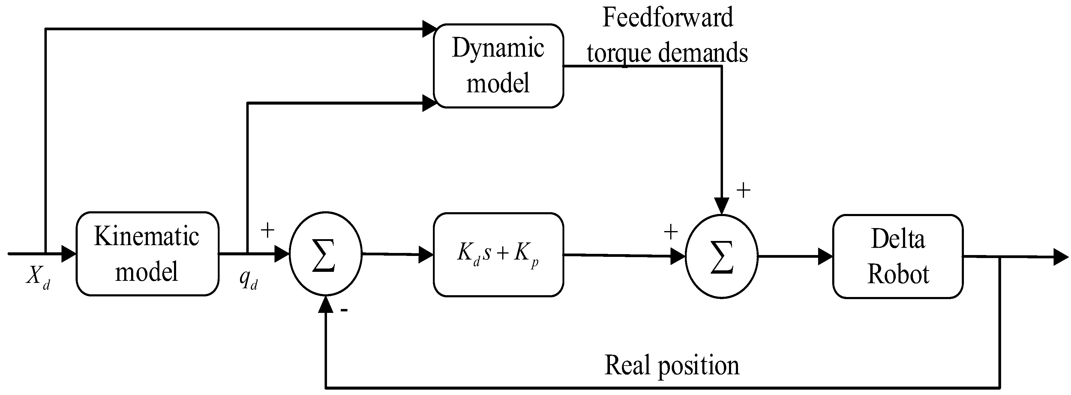
The torque feedforward strategy was implemented successfully on the Delta robot and is sufficient for the implementation of all desired control-algorithm elements [
2]. The scheme used for the control of the Delta robot is shown in
Figure 14. It is composed of a feedforward block of the dynamics model of the Delta robot. Two dynamics models are used, based on Equation (39) and Equation (40), respectively. The control system takes the position of the moving platform (
Xd) as input. The desired joint position (
qd) is obtained using inverse kinematics, and the accelerations are obtained using numerical differentiation of the desired joint angles and moving platform position. The controller is a standard proportional-derivative.
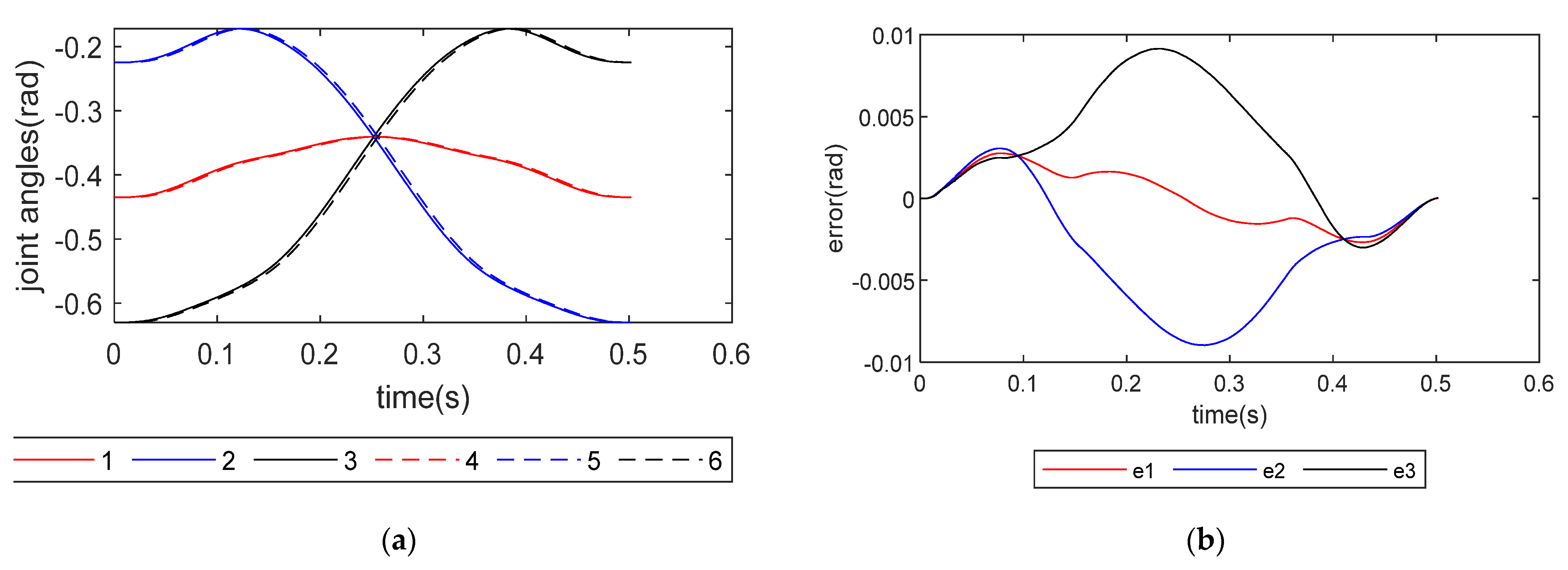
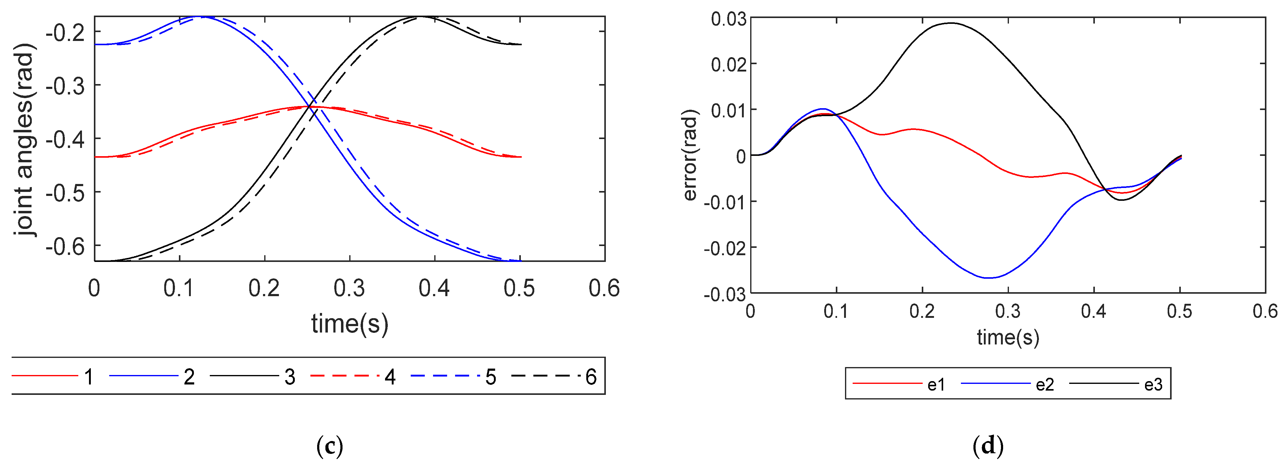
To be able to evaluate the performance of the torque feedforward control algorithm, which uses the dynamics model of the Delta robot with a telescopic rod proposed above, it may be meaningful to compare it with the dynamics model of the Delta robot without a telescopic rod. The tracking errors of the three joints obtained using two different dynamics models are shown in
Figure 15. The tracking error is roughly reduced by half using the dynamics model proposed in this paper.
These results show that the dynamics model of the Delta robot proposed in this paper can better describe the actuator torques, which is beneficial for realizing the precise control of the robot.
6. Conclusions
In this article, dynamics modeling of a Delta robot with a telescopic rod was presented and the proposed dynamics model was applied to the dynamics feedforward control, to verify that the model can describe the actuator torques more accurately. The telescopic rod was regarded as a subsystem of the robot, its degrees of freedom were analyzed, and the kinematics model was deduced under the established generalized coordinate system. The dynamics modeling of the telescopic rod was then evaluated, based on the Euler–Lagrange method and Jacobian matrix of the telescopic rod, which projects forces acting on telescopic rod onto the actuator motors. This dynamics modeling was applied to inertial parameter identification experiments of the Delta robot with a telescopic rod, and the results of the inertial parameter identification experiments were used in the torque feedforward control experiment. The torque feedforward control experiment shows that using the dynamics modeling proposed in this paper can achieve more precise control of the Delta robot with a telescopic rod. Thus, the present study provides a framework for future research on the design and control of this type of parallel robot.
Author Contributions
Conceptualization, S.Z., X.L. and B.Y.; formal analysis, B.Y.; funding acquisition, X.L.; methodology, S.Z.; project administration, X.L.; software, X.H. and J.B.; supervision, X.L.; validation, S.Z., B.Y., X.H. and J.B.; visualization, X.H. and J.B.; writing—review and editing, S.Z. All authors have read and agreed to the published version of the manuscript.
Funding
This research was funded by the National Natural Science Foundation of China (Grant No. 92148301).
Institutional Review Board Statement
Not applicable.
Informed Consent Statement
Not applicable.
Conflicts of Interest
The authors declare no conflict of interest.
References
- Clavel, R. DELTA, A fast robot with parallel geometry. In Proceedings of the 18th International Symposium on Industrial Robots, Lausanne, Switzerland, 26–28 April 1988; pp. 91–100. [Google Scholar]
- Codourey, A. Dynamic Modeling of Parallel Robots for Computed-Torque Control Implementation. Int. J. Robot. Res. 1998, 17, 1325–1336. [Google Scholar] [CrossRef]
- Barreto, J.P.; Corves, B. Resonant Delta Robot for Pick-and-Place Operations. In Advances in Mechanism and Machine Science, Proceedings of the 15th IFToMM World Congress on Mechanism and Machine Science, Krakow, Poland, 15–18 July 2019; Springer: Berlin/Heidelberg, Germany, 2019; pp. 2309–2318. [Google Scholar]
- Honegger, M.; Codourey, A.; Burdet, E. Adaptive control of the Hexaglide, a 6 dof parallel manipulator. IEEE Int. Conf. Robot. Autom. IEEE 1997, 543–548. [Google Scholar]
- Castaneda, L.A.; Luviano-Juarez, A.; Chairez, I. Robust Trajectory Tracking of a Delta Robot Through Adaptive Active Disturbance Rejection Control. IEEE Trans. Control. Syst. Technol. 2015, 23, 1387–1398. [Google Scholar] [CrossRef]
- Zhang, L.; Song, Y. Optimal design of the Delta robot based on dynamics. In Proceedings of the 2011 IEEE International Conference on Robotics and Automation, Shanghai, China, 9–13 May 2011. [Google Scholar]
- Avizzano, C.A.; Filippeschi, A.; Villegas, J.M.J.; Ruffaldi, E. An Optimal Geometric Model for Clavels Delta Robot. In Proceedings of the 2015 IEEE European Modelling Symposium (EMS), Madrid, Spain, 6–8 October 2015. [Google Scholar]
- Zanganeh, K.E.; Sinatra, R.; Angeles, J. Kinematics and dynamics of a six-degree-of-freedom parallel manipulator with revolute legs. Robotica 1997, 15, 385–394. [Google Scholar] [CrossRef]
- Zhu, C.; Wang, J.; Chen, Z.; Liu, B. Dynamic characteristic parameters identification analysis of a parallel manipulator with flexible links. J. Mech. Sci. Technol. 2014, 28, 4833–4840. [Google Scholar] [CrossRef]
- Swain, A.K.; Morris, A.S. A Unified Dynamic Model Formulation for Robotic Manipulator Systems. J. Robot. Syst. 2003, 20, 601–620. [Google Scholar] [CrossRef]
- Pfreundschuh, G.H.; Sugar, T.G.; Kumar, V. Design and control of a three-degrees-of-freedom, in-parallel, actuated manipulator. J. Robot. Syst. 1994, 11, 103–115. [Google Scholar] [CrossRef]
- Lebret, G.; Liu, K.; Lewis, F.L. Dynamic analysis and control of a stewart platform manipulator. J. Field Robot. 2020, 10, 629–655. [Google Scholar] [CrossRef]
- Dimaggio, F.L. Dynamics: Theory and applications. Mech. Mach. Theory 1986, 21, 361–362. [Google Scholar] [CrossRef]
- Liu, M.J.; Li, C.X.; Li, C.N. Dynamics analysis of the Gough-Stewart platform manipulator. Robot. Autom. IEEE Trans. 2000, 16, 94–98. [Google Scholar]
- Masarati, F.P. Real-time inverse dynamics control of parallel manipulators using general-purpose multibody software. Multibody Syst. Dyn. 2009, 22, 47–68. [Google Scholar]
- Caccavale, F.; Siciliano, B.; Villani, L. The tricept robot: Dynamics and impedance control. Mechatron. IEEE/ASME Trans. 2003, 8, 263–268. [Google Scholar] [CrossRef]
- Staicu, S. Recursive modelling in dynamics of Delta parallel robot. Robotica 2009, 27, 199–207. [Google Scholar] [CrossRef]
- Rachedi, M. Model based control of 3 DOF parallel delta robot using inverse dynamic model. In Proceedings of the 2017 IEEE International Conference on Mechatronics and Automation (ICMA), Takamatsu, Japan, 6–9 August 2017; pp. 203–208. [Google Scholar]
- Wu, M.; Mei, J.; Zhao, Y.; Niu, W. Vibration reduction of delta robot based on trajectory planning. Mech. Mach. Theory 2020, 153, 104004. [Google Scholar] [CrossRef]
- Kim, S.H. Dynamics Modeling and Control of a Delta High-speed Parallel Robot. J. Korean Soc. Manuf. Process Eng. 2014, 13, 90–97. [Google Scholar]
- Liu, C.; Cheng, Y.; Liu, D.; Cao, G.; Lee, I. Research on a LADRC Strategy for Trajectory Tracking Control of Delta High-Speed Parallel Robots. Math. Probl. Eng. 2020, 2020, 1–12. [Google Scholar] [CrossRef]
- Wu, L.; Zhao, R.; Li, Y.; Chen, Y.-H. Optimal Design of Adaptive Robust Control for the Delta Robot with Uncertainty: Fuzzy Set-Based Approach. Appl. Sci. 2020, 10, 3472. [Google Scholar] [CrossRef]
- Carp-Ciocardia, D.C. Dynamic analysis of Clavel’s Delta parallel robot. In Proceedings of the 2003 IEEE international conference on robotics and automation (Cat. No. 03CH37422), Taipei, Taiwan, 14–19 September 2003. [Google Scholar]
- Stamper, R.E. A Three Degree Of Freedom Parallel Manipulator With Only Translational Degrees Of Freedom. Diss. Abstr. Int. 1997, 58, 6203. [Google Scholar]
- Codourey, A. Dynamic modelling and mass matrix evaluation of the DELTA parallel robot for axes decoupling control. In Proceedings of the IEEE/RSJ International Conference on Intelligent Robots and Systems. (IROS ’96), Osaka, Japan, 8 November 1996. [Google Scholar]
- Swevers, J.; Ganseman, C.; De Schutter, J.; Van Brussel, H. Generation of Periodic Trajectories for Optimal Robot Excitation. J. Manuf. Sci. Eng. 1997, 119, 611–615. [Google Scholar] [CrossRef]
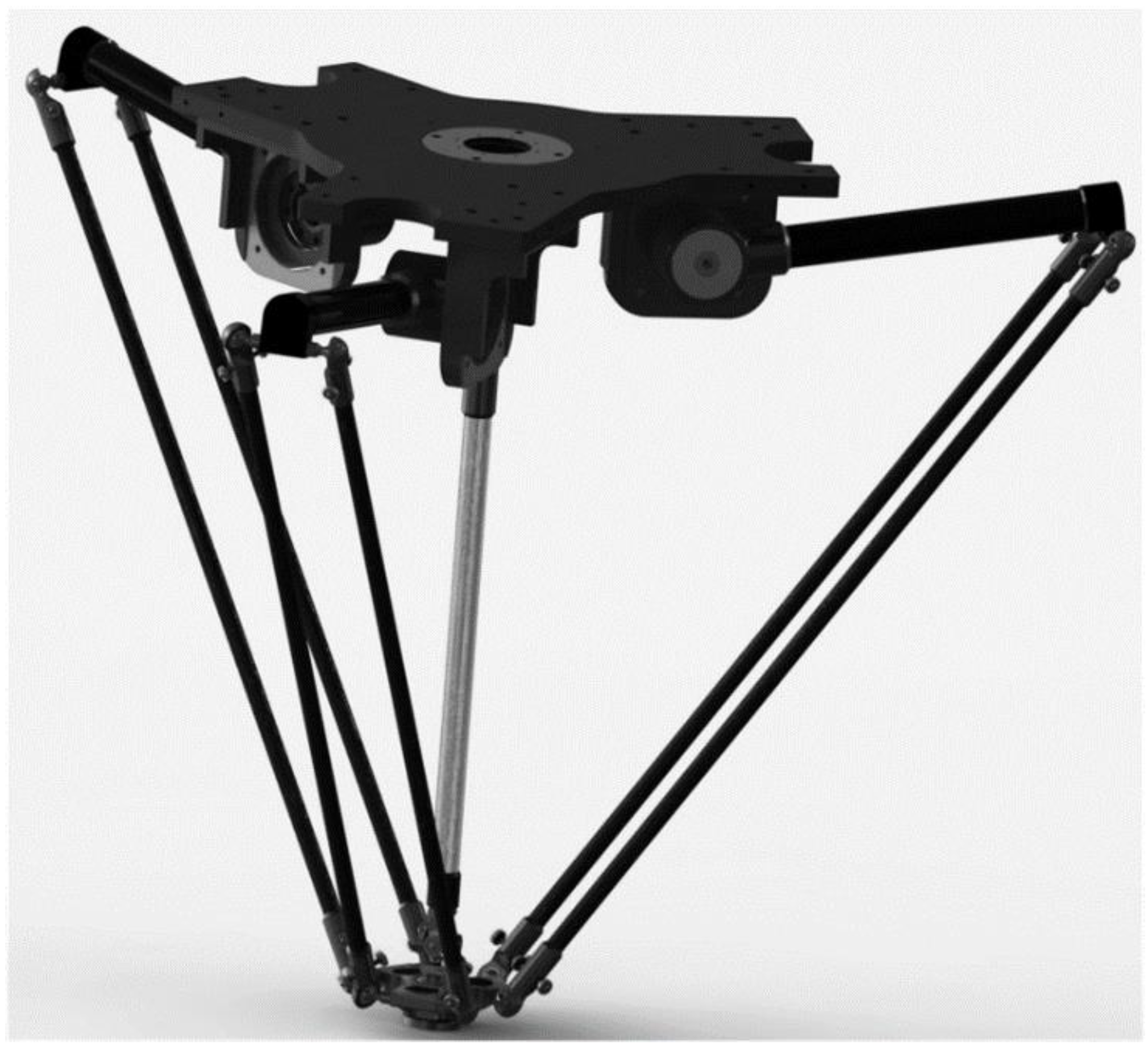
Figure 1.
The mechanical structure of the Delta robot with telescopic rod.
Figure 1.
The mechanical structure of the Delta robot with telescopic rod.
Figure 2.
Schematic of the Delta robot with a telescopic rod: (1) Fixed platform; (2) moved platform; (3–5) upper arms; (6–8) lower arms; (9) telescopic rod.
Figure 2.
Schematic of the Delta robot with a telescopic rod: (1) Fixed platform; (2) moved platform; (3–5) upper arms; (6–8) lower arms; (9) telescopic rod.
Figure 3.
Depiction of leg i.
Figure 3.
Depiction of leg i.
Figure 4.
Generalized coordinate system 1 of the telescopic rod.
Figure 4.
Generalized coordinate system 1 of the telescopic rod.
Figure 5.
Generalized coordinate system 2 of the telescopic rod.
Figure 5.
Generalized coordinate system 2 of the telescopic rod.
Figure 6.
Singularity analysis: (a) planned trajectory between two positions of the platform; (b) planned position of in generalized coordinate system 1; (c) planned position of in generalized coordinate system 2.
Figure 6.
Singularity analysis: (a) planned trajectory between two positions of the platform; (b) planned position of in generalized coordinate system 1; (c) planned position of in generalized coordinate system 2.
Figure 7.
The motion of the moving platform: (a) position; (b) components of the position; (c) components of the velocity; (d) components of the acceleration.
Figure 7.
The motion of the moving platform: (a) position; (b) components of the position; (c) components of the velocity; (d) components of the acceleration.
Figure 8.
Axis variable of telescopic rod: (a) value of axis variable; (b) velocity of axis variable; (c) acceleration of axis variable; (d) the moment of the telescopic rod on the moving platform.
Figure 8.
Axis variable of telescopic rod: (a) value of axis variable; (b) velocity of axis variable; (c) acceleration of axis variable; (d) the moment of the telescopic rod on the moving platform.
Figure 9.
Actuator torques without telescopic rod.
Figure 9.
Actuator torques without telescopic rod.
Figure 10.
Actuator torques with telescopic rod.
Figure 10.
Actuator torques with telescopic rod.
Figure 11.
The Delta robot for experimentation.
Figure 11.
The Delta robot for experimentation.
Figure 12.
The actuator torques with telescopic rod and without telescopic rod (a) 1: the first joint actuator torque with telescopic rod, 2: the first joint actuator torque without telescopic rod; (b) 1: the second joint actuator torque with telescopic rod, 2: the second joint actuator torque without telescopic rod; (c) 1: the third joint actuator torque with telescopic rod, 2: the third joint actuator torque without telescopic rod.
Figure 13.
Comparison between the predicted and real actuator torques (a) 1: predicted actuator torque of first joint, 2: real actuator torque of first joint; (b) 1: predicted actuator torque of second joint, 2: actuator torque of second joint; (c) 1: predicted actuator torque of third joint, 2: actuator torque of third joint.
Figure 14.
Feedforward control of Delta robot.
Figure 14.
Feedforward control of Delta robot.
Figure 15.
The joint trajectory and tracking errors: (a) actual joint angle and planned joint angle, which uses proposed dynamics modeling; (b) tracking errors of using proposed dynamics modeling; (c) actual joint angle and planned joint angle, which use traditional dynamics modeling; (d) tracking errors of using traditional dynamics modeling. Numbers 1, 2 and 3 are planned joint angle of joints 1, 2 and 3; 4, 5 and 6 are actual joint angles of joint 4, 5 and 6; e1, e2, and e3 are tracking errors of joints 1, 2 and 3.
Table 1.
Mechanical parameters of Delta robot.
Table 1.
Mechanical parameters of Delta robot.
| Length of upper arm | 385 mm |
| Length of lower arm | 900 mm |
| Radius of fixed platform | 200 mm |
| Radius of moving platform | 60 mm |
Table 2.
Identified inertial parameters.
Table 2.
Identified inertial parameters.
| The mass of upper arm (kg) | 0.524 |
| The mass of lower arm (kg) | 0.433 |
| 0.0886 |
| 0.451 |
| 0.832 |
| The mass of upper rod (kg) | 0.134 |
| The mass of lower rod (kg) | 0.416 |
| Damping ratio (Ns/m) | 0.233 |
| Publisher’s Note: MDPI stays neutral with regard to jurisdictional claims in published maps and institutional affiliations. |
© 2022 by the authors. Licensee MDPI, Basel, Switzerland. This article is an open access article distributed under the terms and conditions of the Creative Commons Attribution (CC BY) license (https://creativecommons.org/licenses/by/4.0/).


