1. Introduction
The control of robotic manipulators is strongly linked to the study of their motion. Forward kinematics refers to the process of determining the position and orientation of a robotic end effector with known joint parameters [
1]. Although by definition, the position and orientation of all links are not required to solve a forward kinematics problem, in this paper, the goal is to obtain the complete definition of all the link’s orientations and positions to fully describe the robot’s 3D configuration.
The most used method for the kinematic analysis of robotic manipulators is the Denavit–Hartenberg parameters [
1]. This approach concisely allows the characterization of each link using four parameters, providing a compact definition of a robot’s kinematic structure. However, this methodology has two drawbacks. The first is fixing the choice of axes, which is defined by the orientation of the joints. This prevents researchers from picking a more natural axes orientation based on the configuration of the kinematic links, where each axis could be associated with a specific physical meaning (for example, using the
z-axis for heights, or the length of parts). The second is that calculations are made based on homogeneous transformations. These [4 × 4] matrices define rotations and translations in a single operation, however, the last line of the matrix does not contain any relevant information, being constituted by 0 s and 1 s to allow algebraic operations. These additional multiplications reduce the computational efficiency of the forward kinematics analysis. A known solution to this problem is to divide translations and rotations into different operations [
2].
This paper presents an alternative generalizable methodology that intends to deal with both of these limitations. This method is based on a recursive algorithm that builds a 3D model of the robot from its base, to its end-effector. The algorithm progresses along the kinematic chain, determining the rotation matrix that defines the orientation of each link i. This matrix is obtained from the orientation of the preceding link , and the relative orientation between the current link and its predecessor . The rotation between consecutive links is defined using Euler Angles. After the orientation of a link is determined, its position is obtained from the joint coordinates resulting from the 3D modeling of its predecessor . This process provides the necessary information for the definition of the geometry of each of the robot’s links, the determination of the position and orientation of these links, and their three-dimensional representation.
This method was implemented in Python using the numpy library for matrix and trigonometry operations, and Matplotlib for the 3D plotting of the robot’s points to allow the observation of its behavior in a 3D graphical interface. For validation, the algorithm was used to analyze CHARMIE [
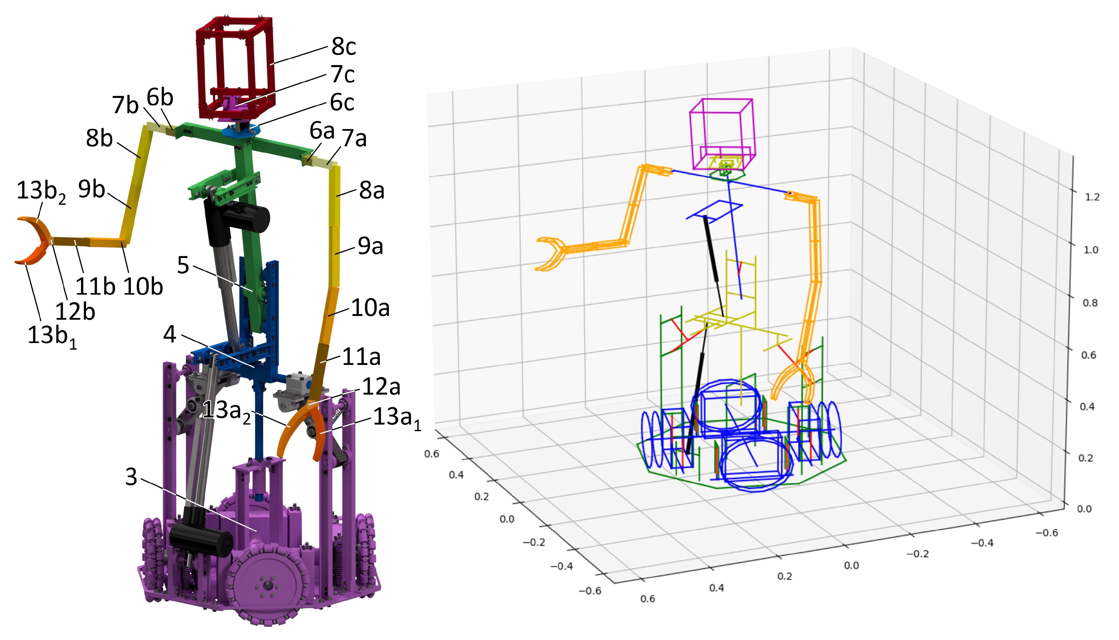
3], a human-inspired mobile manipulator robot (
Figure 1). This robot also serves as an example throughout the paper to better explain the developed algorithm.
In
Figure 1 the robot’s base is shown as a single kinematic link. At this stage, the behaviour of the omnidirectional locomotive system was not considered (the wheels and suspension system are represented, but they do not move in relation to the robot). Instead, as a simplification, the robot was modeled as having its base sliding (in the
x and
y axes) about the floor using two linear actuators, and rotating (around the
z-axis) using a revolute actuator. The arms and end-effector shown in the CAD model are mere placeholdes, since one of the results from this kinematic analysis is the study responsible for dimensioning them.
The main contribution of this paper is the presentation and explanation of a methodology for the study of forward kinematics. This methodology produces a computationally defined 3D model of a robot, which can be used for a set of relevant analyses in the field of robotics. Two examples of these applications are the studies being conducted in CHARMIE, where this kinematic model is being used not only as the starting point to build a simulation environment for the training of a neural network to control the robot’s motion and trajectories, but also for multibody dynamics analysis, where the recursive Newton Euler algorithm described in [
4] is used to compute the robot’s inverse dynamics. The cited Newton Euler algorithm is fully compatible with the methodology presented in this paper, directly using the information obtained from it (positions, configuration of each link, and orientations between consecutive bodies in the form of rotation matrices).
To fully describe and validate this methodology, the paper is structured as follows: in
Section 2 a Literature Review is provided, where several methods for the 3D representation of rotations are listed and described, followed by a justification of the choice of method for this paper;
Section 3 presents, formulates, explains and describes the recursive algorithm developed in this paper, dividing it into three simple steps;
Section 4 provides an example of application of this methodology, using it to build a 3D model of the CHARMIE mobile manipulator, defining the robot and explaining how the modeling of some of its particularities was dealt with;
Section 5 finishes the paper discussing results and commenting on possible future works.
2. Literature Review
The forward kinematic analysis can be tackled as a matter of obtaining the 3D configuration of a group of bodies (links) from a set of known conditions (joint parameters). It is possible to fully define a rigid body in 3D space with its orientation and the coordinates of one of its points. The position of a point, in Euclidian space, is easily described using three coordinates: x, y, and z, however, defining three-dimensional rotations, often denoted SO(3), is a more complex topic. Several formalisms have been developed for this purpose, they can be used together, and the conversion between them is a well-studied process. In this Literature Review, some of the main notations used in the field of robotics for the description of 3D rotations are listed and described, followed by a few examples of works that use them. This section finishes by presenting and justifying the method chosen for this paper.
Rotation Matrices are [3 × 3] matrices commonly used to define the rotation between two coordinate frames
i and
j. A rotation matrix
describes the rotation from frame
i to frame
j. These matrices represent the dot product between the basis vectors
and
of the two considered frames [
2]. When multiplying the coordinates of a point
P with the rotation matrix
, the result is a transformation which follows the rotation defined between frames
i and
j. This can be used to convert the coordinates of points between references with different orientations. Rotation matrices can be combined by simple matrix multiplication (
=
), allowing the representation of a limitless sequence of rotations. Due to the simplicity of their manipulation, they are often used to describe rotations obtained from the application of different formalisms, such as Euler Angles [
5].
The Denavit—Hartenberg convention is one of the most used notations for the kinematic analysis of serial manipulators. Four parameters are used to describe the transformations between each consecutive element of the kinematic chain:
and
describe the link’s length and twist;
and
describe the joint’s offset and angle [
6]. To apply this method, a set of reference axes are attached to the links of the kinematic chain. The definition of these references is based on the orientation and position of the joints and follows a set of rules and conventions usually described by a set of steps (such as presented in [
1]), to guarantee the cohesion of the resulting Denavit–Hartenberg parameters. From these four parameters, a [4 × 4] homogeneous transformation matrix is constructed containing information regarding the rotation and translation between each consecutive pair of links. These matrices can be combined, multiplied, and easily manipulated like the aforementioned rotation matrices. Mostly used for serial manipulators, this method is highly advantageous due to: representing robot kinematics in a compact form; producing consistent results thanks to the rigid and detailed methodology; the vast amount of algorithms and works already developed for it. Examples of papers using this notation are available in [
7,
8,
9].
Euler angles represent any rotation of a three-dimensional object as a sequence of three consecutive rotations. These rotations can be extrinsic (around the fixed motionless original
axes) or intrinsic (around the rotating coordinate axes of the considered body). The sequence of rotations uses proper Euler angles if the first and third rotations are around the same axis, or Tait–Bryan angles if all three rotations are around different axes. Depending on the research field, different authors use different names, and axes, to define Euler angles, so it is important to verify the nomenclature used in each work. There are two well-known limitations related to the use of Euler angles. The first is the Euler Angle singularity, which occurs when the angle of the second rotation is
or
. In these cases, the first and third Euler Angles can vary independently, both controlling the same degree of freedom, resulting in an infinite number of possible combinations for defining a single orientation. The second problem, gimbal lock, also occurs for the same values of the second rotation. Due to two rotation axes being aligned, a degree of freedom is lost, which prevents the system from immediately doing determined motions. These limitations can be corrected, or become severe problems, depending on the intended applications. An explanation of these limitations, and ways to address them, is available in [
10]. Some examples of works using the Euler-Angles notation are [
11,
12,
13].
A quarternion is a four-dimensional vector, represented by 4 scalar entities, which can be harnessed to compute rotations on points and vectors in three dimensions. They are one of the major alternatives to rotation matrices, and are commonly used due to their high efficiency in computer calculations and their ease of interpolation. They also avoid both previously described problems related to Euler Angles. It should be noted that quarternions have their limitations, such as a reduce in efficiency when calculating the rotation of a vector [
14]. The formulas required for the use of quaternions are well-known, but the understanding of these formulas, and underlying principles, is complex [
14]. Some works allow a deeper understanding of quaternions, such as the paper [
14], and the books [
15,
16]. A survey is presented in [
17] which reviews and compares methods for the computation of quaternions from rotation matrices. Quaternions are used in the following works: [
18,
19].
Another possible method for the computational analysis of multi-body kinematics is screw theory (usually alongside Lie groups). In screw theory, two three-dimensional vectors are used to represent: the position and orientation of a rigid body; the linear and angular velocity of a rigid body; a force and a couple [
20]. The two vectors define the Plücker coordinates of a line in space (the position and direction of the screw axis), the magnitude of the screw, and its pitch. These four factors completely define a screw [
20]. Using screw theory in conjunction with Lie algebra se(3), associated with Lie group SE(3) [
21], it is possible to develop recursive algorithms that solve the kinematics of multi-body problems with high computational efficiency [
22]. Some examples of works that use Screw Theory are [
23,
24,
25].
Regarding the methodology used in this paper, the rotation between two consecutive bodies is defined using ZXZ intrinsic Euler angle rotations. These rotations can be easily converted into other formalism [
5] (such as rotation matrices that can be more conveniently manipulated), the comprehension of their geometry is straightforward, and they allow a free choice of local axes for each link (it may become beneficial to program a constant rotation to guarantee convenient axes orientation). Since most used joints in robotics rotate around a single axis (revolute joints), problems regarding singularities and the gimbal lock are easily avoided with the choice of local orientation. More complex joints (such as spherical joints) can be modeled using a single complex Euler angle rotation, or as a sequence of rotations with one degree of freedom around the same point. The rotations obtained from the Euler angles are converted into rotation matrices, and all following mathematical operations are made using said matrices.
3. Recursive Algorithm for the Computation of Forward Kinematics
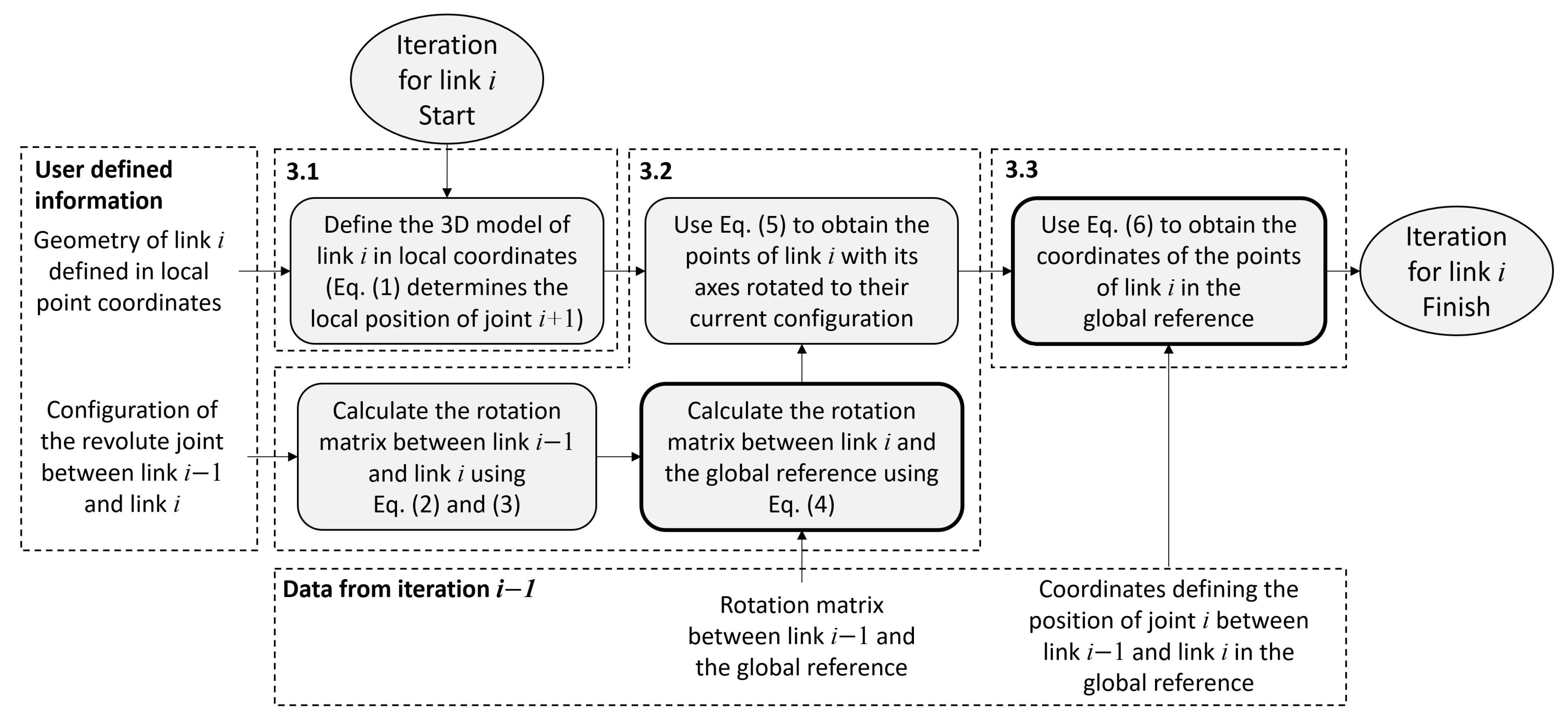
The structure of the developed recursive forward kinematics algorithm is illustrated in
Figure 2. This algorithm computes the positions of the robot’s links from known joint configurations. After running this algorithm from link 0 (the global reference) to the robot’s end-effector, the coordinates and orientations of all bodies in the kinematic chain are fully defined. The calculations are made sequentially, using information regarding both the current link
i and the previous link
.
In
Figure 2, the boxes with stronger outlines represent the steps where the orientation (in the form of a rotation matrix) and position (in the form of coordinates) of the link are defined. With this information, additional data (such as linear and angular velocities and accelerations) can be calculated.
The algorithm is divided into three main steps, which are described in greater detail—accompanied by an example—in the following subsections:
Definition of the geometry of link i;
Rotation of link i into its current orientation;
Translation of link i into its current position.
The following terms are used to define and name points and axes in this paper:
—The local coordinate axis of link i;
—The coordinate axis of link i after considering the link’s rotation to its actual orientation;
—The global reference axis;
—The origin of link i, placed on the connection point between link i and link ;
—The connection point between link i and link ;
—The link’s center of mass (important for posterior dynamics calculations);
—The position of the joint between link i and link considering a linear joint displacement of 0.
—Refers to all points of link i.
If the joint after a link is revolute, point
is fixed and equal to
. However, if this joint is prismatic, this point will move based on the position of the linear actuator. These calculations must be made in local coordinates when analyzing link
i, so that when iteration
begins, the position of the origin of link
in global coordinates is already known. This is done using the equation:
where
is the linear displacement of the prismatic joint between link
i and link
, and
the unit vector defining the orientation of this prismatic joint in relation to the
local axes.
The rotation matrix associated with an intrinsic ZXZ Euler rotation, defined by the angles (
,
, and
), is obtained from [
5]:
where
c represents a cosine function,
s a sine function, and the indexes 1, 2, and 3 the corresponding angles (angle of the 1st rotation around the
z-axis, angle of the 2nd rotation around the new
x-axis, angle of the 3rd rotation around the
z-axis after the first two rotation are applied).
If the local coordinate axes for two consecutive links are aligned when the associated joint rotation angle
is 0, the rotation matrix
between them can be directly determined using:
in this equation, the orientation of the joint axis and the joint rotation angle
are used to define the inputs for Equation (2).
The orientation of link
i, defined by
, is then determined using:
where the rotation matrix
, which defines the orientation of link
in relation to reference 0 (already determined in iteration
of the algorithm), is multiplied by the rotation matrix
determined in the previous Equation (3).
The
points of link
i rotated into its current orientation (expressed in the
axes) are obtained using:
where the rotation matrix
is used to rotate the
points in the local axes of link
i around point
.
A last equation then determines the coordinates of the points
of link
i expressed in the
global axes:
where the coordinates of point
(determined in the previous iteration of the algorithm) are used to translate the
points of the rotated axes of link
i into their correct position and orientation.
In particular cases, a joint may not be directly actuated, and additional calculations are required based on the geometry of the robot. Examples of this are given in
Section 4.2.
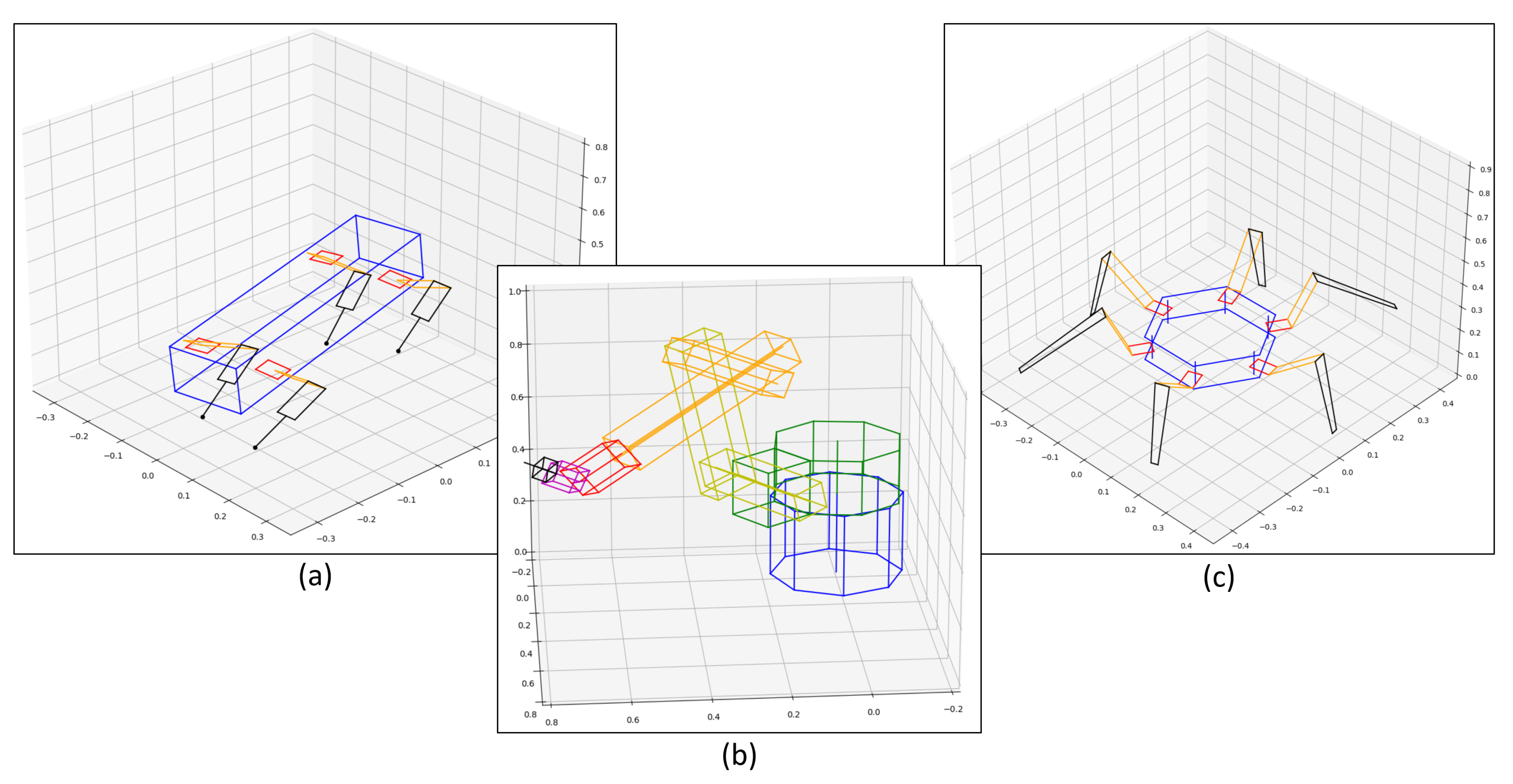
This simple algorithm can model robots with different configurations and purposes. Besides CHARMIE, studied in the following sections,
Figure 3 shows three examples of kinematic models obtained using this method: (a) a mobile quadruped robot similar to SPOT from Boston Dynamics [
26]; (b) a fixed serial manipulator similar to KUKA KR 500-3 [
27]; and (c) a mobile hexapod similar to the one presented in [
28].
These three models were made as follows:
Quadruped robot—First, the main body of the robot was created. Then, a single leg was modeled. The leg model was replicated four times, and each of them was placed in its respective connection point to the body (a constant rotation altered the origin orientation between legs on the left and the right side of the robot). This resulted in a fully defined kinematic model controlled by 12 joint angles (3 for each leg). To study the robot’s locomotion, the model can be placed in a simulation environment that considers the dynamic interactions between the feet and the floor.
Fixed serial manipulator—To build this model, each body was created in local coordinates, and then the robot was assembled with the proposed algorithm. This model is controlled by the angles of the 6 revolute joint. This analysis is similar to problems commonly tackled using Denavit-Hartenberg parameters.
Hexapod robot—Modeling the hexapod was similar to the quadruped robot, with the main difference being the use of a rotation between each leg in relation to the body. The resulting kinematic model is controlled by 18 joint angles (3 for each leg). Similar to the quadruped robot, after interaction with the floor is defined, this model can be used to study locomotion.
The use of this algorithm provides the same advantages for the study of these three robots as for CHARMIE. Besides the resulting models being compatible with other methods, they are inherently parametric and modular. As an example, this allows doing a parametric study of the limb length for the mobile robots to minimize actuator torque or maximize locomotion velocity. All shown models can also be used for machine learning applications.
The algorithm’s behaviour will now be explained and illustrated by using it to model the head (link
) of the CHARMIE robot. At this iteration, the algorithm has already finish running for all links leading to link
, which produces the model shown in
Figure 4.
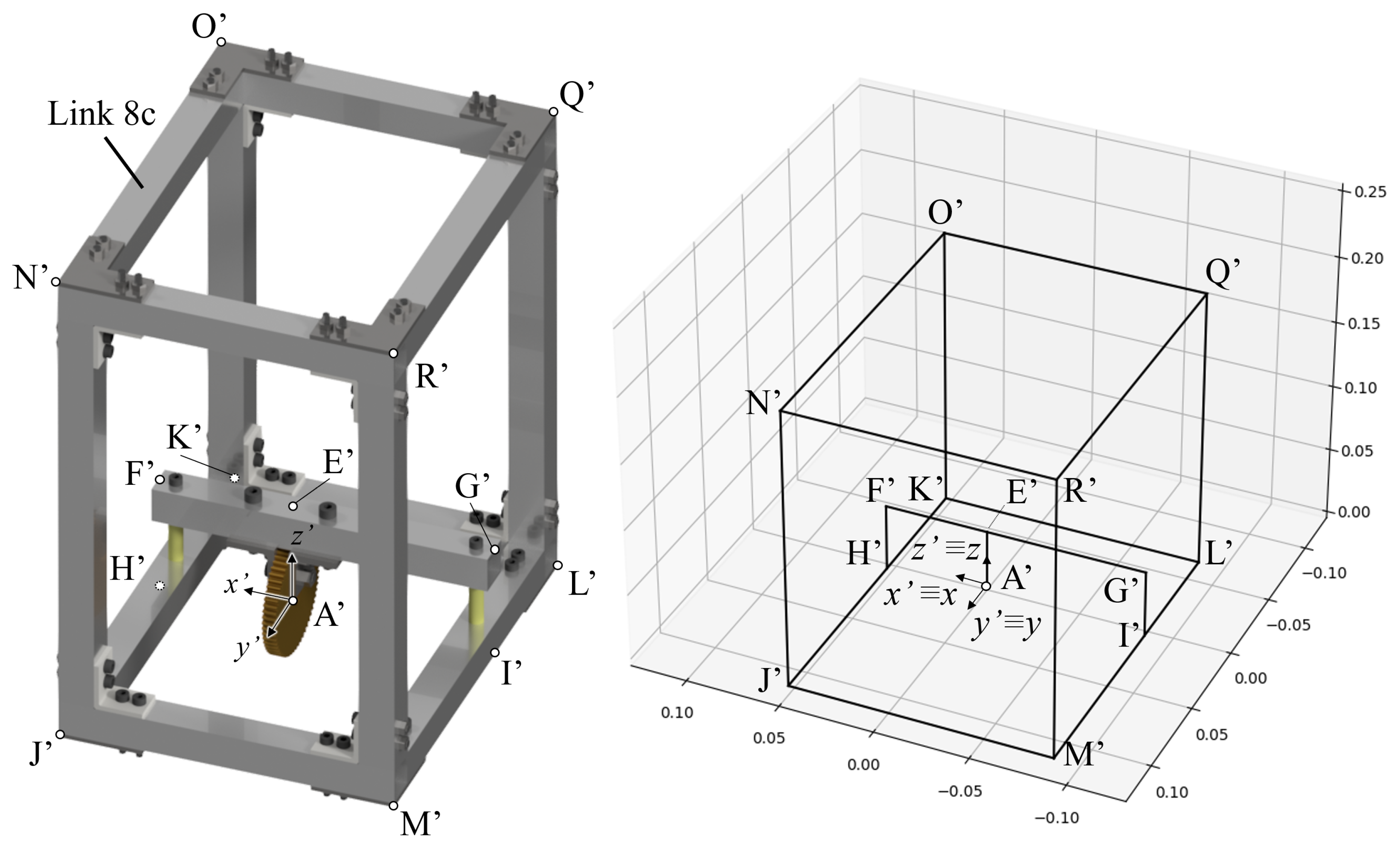
3.1. Modeling Link i in Its Local Coordinates Axis
The first step is the construction of a 3D model of the link being analyzed in its local coordinates. The origin of each link, identified as point , is placed on the point where link i is connected to link . The geometry of each link can be defined by any number of points (or other methods, such as surfaces or equations).
A coherent choice of local axes orientation for the 3D models facilitates the implementation of the algorithm. In this example, represents the positive height of complex parts, or the length of tubes, the positive points to the front of the part, and the axis points from left to right.
To demonstrate this step,
Table 1 shows the local coordinates of the CHARMIE robot’s head (link
). Since this is the end of a kinematic chain, point
corresponds to the end-effector (in this example, it is a point in the top of the robot’s head, but the position of a camera could also be considered). Equation (1) defines the position of
being the same as
because the joint after link
has no motion (in this case, it is a fixed point).
Figure 5 shows the 3D model obtained from the points of
Table 1. The head is represented in a 3D plot by drawing lines between the relevant points. Points
to
were not illustrated since they are only relevant for internal calculations, not for the graphical representation of the head.
It should be noted that if the goal is to obtain the solution of the forward kinematics with maximum computational efficiency, each link can be simplified to only contain points and (when the following joint is revolute, only is needed).
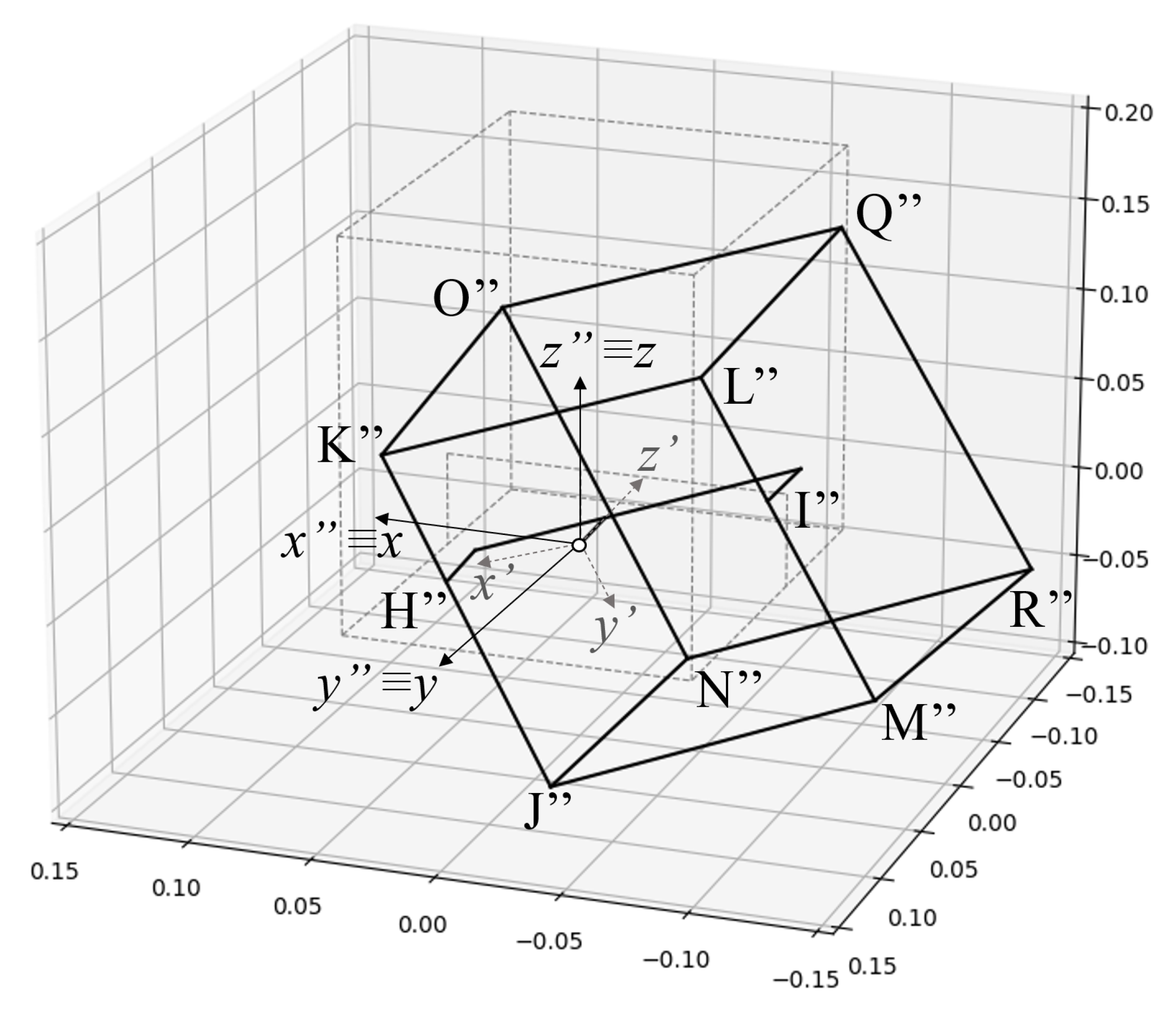
3.2. Rotating Link i to Its Current Orientation
In the second step of the algorithm, the orientation of link i is determined. In this work, intrinsic proper Euler rotations along the ZXZ axes are used to describe the rotation between each pair of consecutive links.
Since the local axes were chosen fulfilling the conditions for Equation (3), it can be used together with Equation (2) to obtain the rotation matrix . If the axes were not aligned, constant angles could be added to Equation (3) to include the change of orientation.
Knowing the orientation of link about the global reference , which was determined in the previous iteration of the algorithm, and the rotation between link and link , the orientation of link is obtained using Equation (4).
With the orientation of link determined, it is now possible to rotate it to its current configuration. A new auxiliary reference, , is created to represent link after its rotation. This rotation is applied to all points of the link using Equation (5).
Figure 6 shows the robot’s head, and its corresponding points, after being rotated to a specific configuration. This orientation is calculated using data resulting from all iterations until the current one is reached, indirectly utilizing information from the rotation of all revolute joints along the kinematic chain.
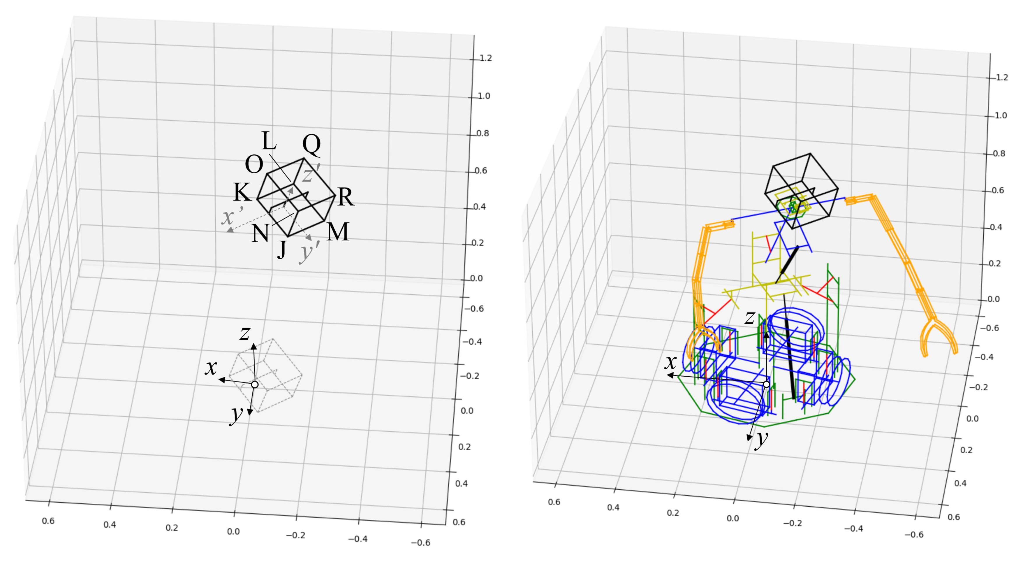
3.3. Moving Link i to Its Current Position
With link in its correct orientation, the only step left is the translation to its current position. The coordinates of the connecting point between link and link in the xyz global axes were already determined in iteration of the algorithm. Since the model of link was built around this same connection point in its local reference (), the global coordinates are obtained by adding the coordinates of point to all previously rotated points using Equation (6).
The coordinates of
are used for all
points since they all follow the same translation. With this step finished, link
becomes modeled in its current position with its current orientation, as shown in
Figure 7.
4. Application of the Algorithm for the CHARMIE Robot
To validate the proposed algorithm, and provide a further understanding of how it is applied to a practical example, this section describes the process of using it to model CHARMIE [
3], a human-inspired mobile manipulator robot (
Figure 1).
The application of the algorithm to an ongoing project also proved its usefulness by successfully serving as a basis for two studies:
Develop a 3D environment for multibody dynamic analysis—Using the recursive Newton-Euler algorithm for the inverse dynamics analysis presented in [
4], together with the algorithm described in this paper, a 3D multibody dynamic analysis of the CHARMIE robot has been built. This study was fundamental for the mechanical project of the robot and the choice of actuators. Results from this methodology were validated both using benchmarks from literature, and comparing results to other multibody simulation software (WorkingModel4D and CoppeliaSim).
Analyse and train neural network solutions for trajectory control—The forward kinematic analysis defines the robot’s configuration as a function of its joint positions. After defining limits for the joints, and a set of conditions that determine the success and failure of a trajectory generation (example: a collision is a failure, and getting into an intended position is a success), a neural network can be trained to control the joint actuators to find optimal trajectories. By hiding the visual interface of the developed algorithm, high computational efficiency is achieved, optimal for neural network training. By also including contact between bodies (using, for example, the mathematical models in [
29]) this method will be used to train CHARMIE for manipulation tasks, such as picking and placing of objects.
In the following subsections, CHARMIE’s kinematic structure is described, followed by an explanation of the auxiliary calculations required to both correctly model the robot’s forward kinematics, and to extract data regarding the configuration of components that were not modeled directly. This section finishes by presenting a comparative study, made using WorkingModel4D, to validate the obtained results.
4.1. Definition of the Robot’s Kinematic Chain
The first step for analyzing CHARMIE was organizing its kinematic structure by defining and naming its links and joints. The result from this process is shown in
Figure 8, which schematically represents the kinematics of the robot. The manipulator was modeled as a single serial kinematic chain from the global reference to its upper body and then split into three different serial kinematic chains, one for the left arm (chain
a), one for the right arm (chain
b), and one for the head (chain
c). The end of both arms also splits into the two halves of the end effectors claws. The motion of both halves of each claw is controlled by a single actuator (joint
and joint
).
Next, all information required to run the algorithm was prepared and computed. This includes the coordinates of the points considered for each link in their local coordinates, and the
matrices obtained using Equation (3). This information is listed in
Table 2. For simplicity, only the coordinates of points
(enough to model the robot’s kinematics) are shown. Since link 5 is connected to three different links, it has three different
associated. Despite being connected to two links, links
and
have a single
due to both halves of the end effector having the same origin. Links
,
,
,
, and
have no
because they are end effectors, not connected to any following link.
This information (and the coordinates of the other points to draw each link) was enough to build the model of
Figure 1. The only exceptions were Joints 4 and 5 which, due to not being directly actuated, required additional calculations.
4.2. Auxiliary Calculations for Complex Joints
The recursive algorithm presented in
Section 3 can model any link from known joint values. However, in some practical examples, joints are not directly actuated, and it is necessary to establish the correspondence between the actuator position and the joint value. This happens in two joints of CHARMIE: joint 4, a prismatic joint actuated indirectly by a linear actuator; and joint 5, a revolute joint controlled by a linear actuator. Since these calculations can be applied to similar situations in other robots, they are explained in detail.
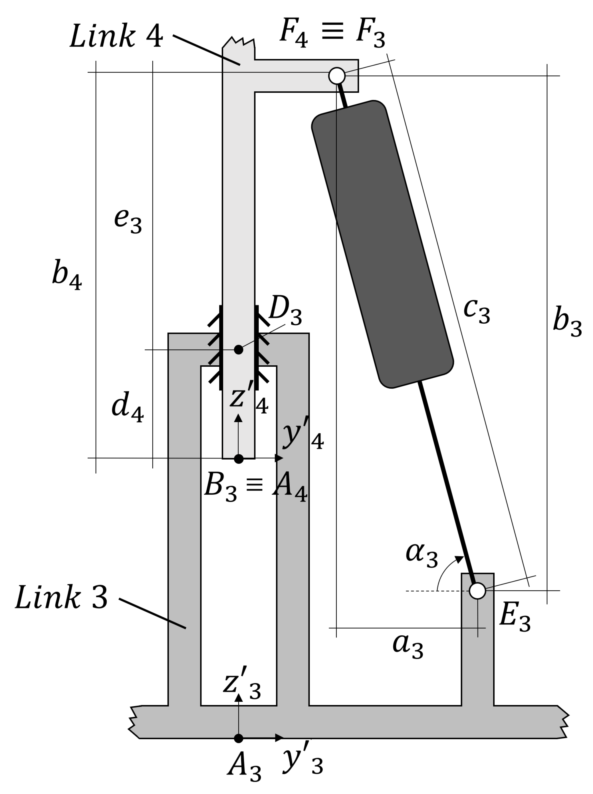
4.2.1. Joint 4
Joint 4 of CHARMIE is a prismatic joint indirectly actuated by a linear actuator. The goal is to establish a relation between the length of the linear actuator
and the linear displacement of joint 4
. The relevant geometric features for this calculation are shown in
Figure 9.
For these calculations, global coordinates from link 4 cannot be used (because at this stage of the algorithm, this link is not modeled yet), but the local coordinates can since they only depend on the link’s geometry, which is constant. First, an auxiliary point
was included in link 3, which corresponds to the endpoint of the linear actuator. The
coordinate of this point is fixed, and can be used to determine
using the expression:
With this value and the current lenght of the actuator
, the auxiliary angle
can be determined:
This angle allows the height
to be obtained:
which then allows the height of the auxiliary point
to be determined:
With
determined, and
being a known and fixed point,
is calculated using:
The height
is only dependant on the geometry of link 4, and is calculated using:
It then becomes possible to calculate
using:
By combining Equations (7)–(13), the relation between
and
is obtained, resulting in equation:
Point
was removed from this equation since its value is 0. To allow reproducibility of results, the required geometric values for this step are shown in
Table 3.
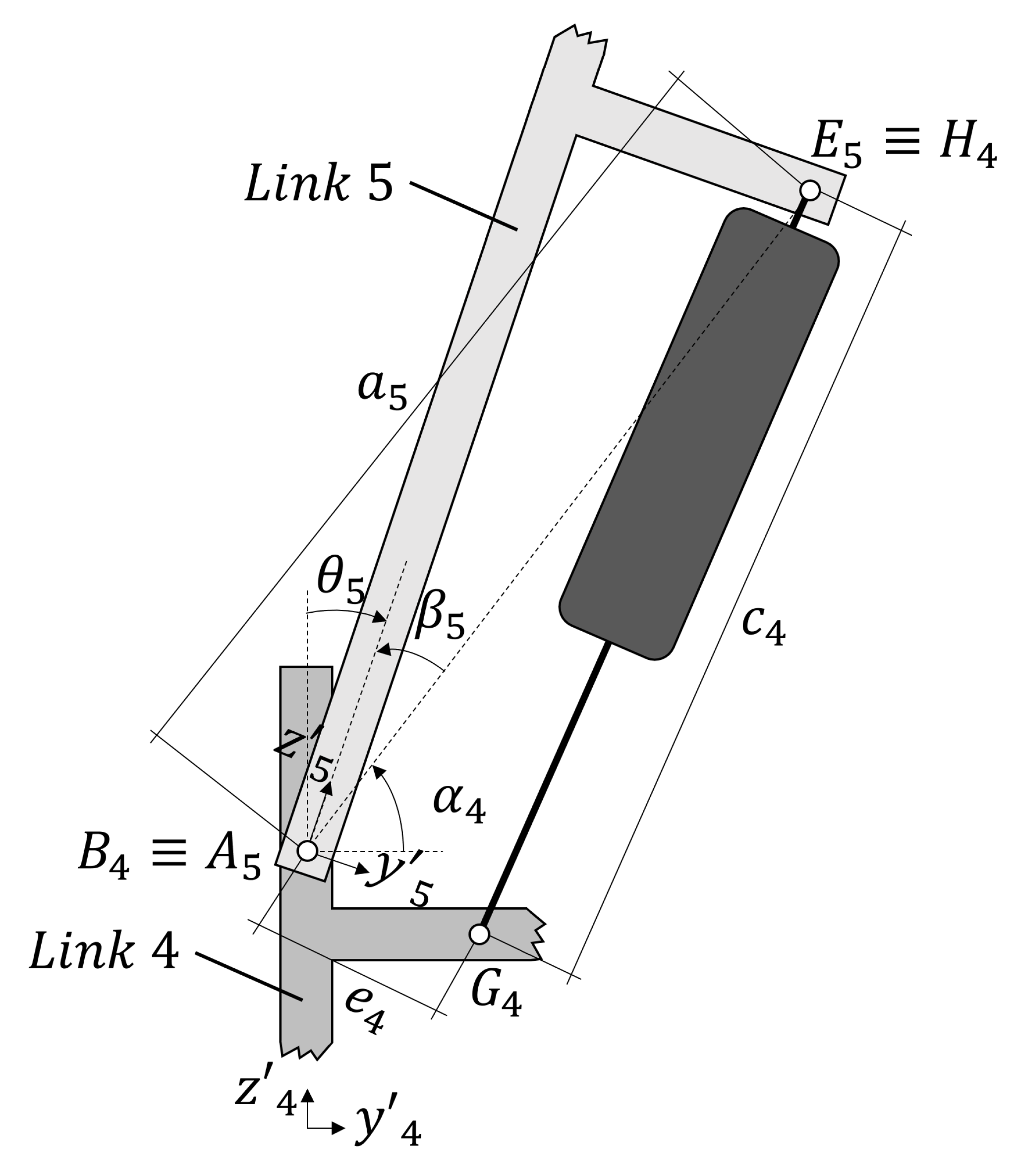
4.2.2. Joint 5
Joint 5 of CHARMIE is a revolute joint actuated by a linear actuator between links 4 and 5. The goal is to establish the relation between the configuration of the linear actuator
and the rotation of the joint
. The geometric features used in this calculation are represented in
Figure 10.
As in the previous example, only local coordinates (related to the parts’ geometry) or lengths (constant regardless of the chosen reference) are used. The angle
can be determined from two auxiliary angles,
and
, using the expression:
where
can be calculated using:
and
using the expression:
The points required for obtaining are only dependant on the geometry of link 5, therefore, they can be determined directly. However, requires the coordinates of point , which are dependant on the geometry of link 4, the geometry of link 5, and the length of the actuator .
The coordinates of
were calculated as the intersection between two circumferences, one with its center on point
and radius
, and the other centered on point
with radius
. Radius
is obtained from the actuator length, and
from the expression:
To calculate the intersection between two circumference, the distance between their centers
is also needed, given by the expression:
To facilitate the formulation of the intersection, two auxiliary mathematical parameters were used. The first is
, given by the expression:
and the second is
, calculated from the expression:
The coordinates of
can then be determined using the pair of equations:
By combining Equations (15)–(23), the expression establishing the relation between and is obtained. This expression is not be presented in its extended form due to its size, which would hinder its comprehension.
To allow the results to be reproducible,
Table 4 shows the coordinates of all geometric features used for this calculation.
4.3. Auxiliary Calculations to Extract Relevant Data from the Model
After the model is obtained, a set of data not modeled directly can be obtained from it.
One example for this, in the CHARMIE robot, is the configuration of the springs included between links 4 and 5. The connection points between these springs,
and
, are placed on the local coordinates, but the global configuration of the spring is not explicitly defined. After the recursive algorithm runs, the spring length
can be easily obtained by calculating the distance between the two connection points
and
in the global coordinate reference, as shown in the following equation:
Any angle
can also be calculated by defining a triangle using three distances:
;
;
. The value of these distances can be determining using Equation (24), and the value of the angle is then calculated by applying the law of cossines in the form:
where
is the opposite side of the triangle to the internal angle being calculated.
Using integration, it becomes possible to evaluate problems over time. A possible method for obtaining the angular velocity, angular acceleration, and linear acceleration of all links is to use the forward iterations of the recursive algorithm from chapter 7.5.2 of [
4]. The inputs of this method are the information obtained in this algorithm (rotation matrices and coordinates of points
,
and
), and the known inputs from the forward kinematics analysis (joint orientation, position, velocity, and acceleration).
4.4. Validation of Results
To validate the developed algorithm, the CHARMIE robot was also modeled in the multibody simulation software WorkingModel4D. The same problem, a simple motion that requires the movement of all joints, was solved using both methods to compare and verify the results.
All actuators started with a position/angle of 0, except for
and
, actuated by the linear actuators
and
, which started in the positions
mm and
mm. All joints were defined with a constant velocity. The angular velocity considered for the directly actuated revolute joints was
rad/s, and the linear velocity for the linear actuators 5 mm/s. The three exceptions were joints
and
, both with an angular velocity of
rad/s, and the linear actuator
, with a linear velocity of
mm/s. To analyse a single set of coordinates, the claw end effectors were replaced with a point at their center—this corresponds to changing
Table 2 by: removing rotations
and
; and changing the value of
and
to
. The robot was simulated under these conditions for a period of 20 s.
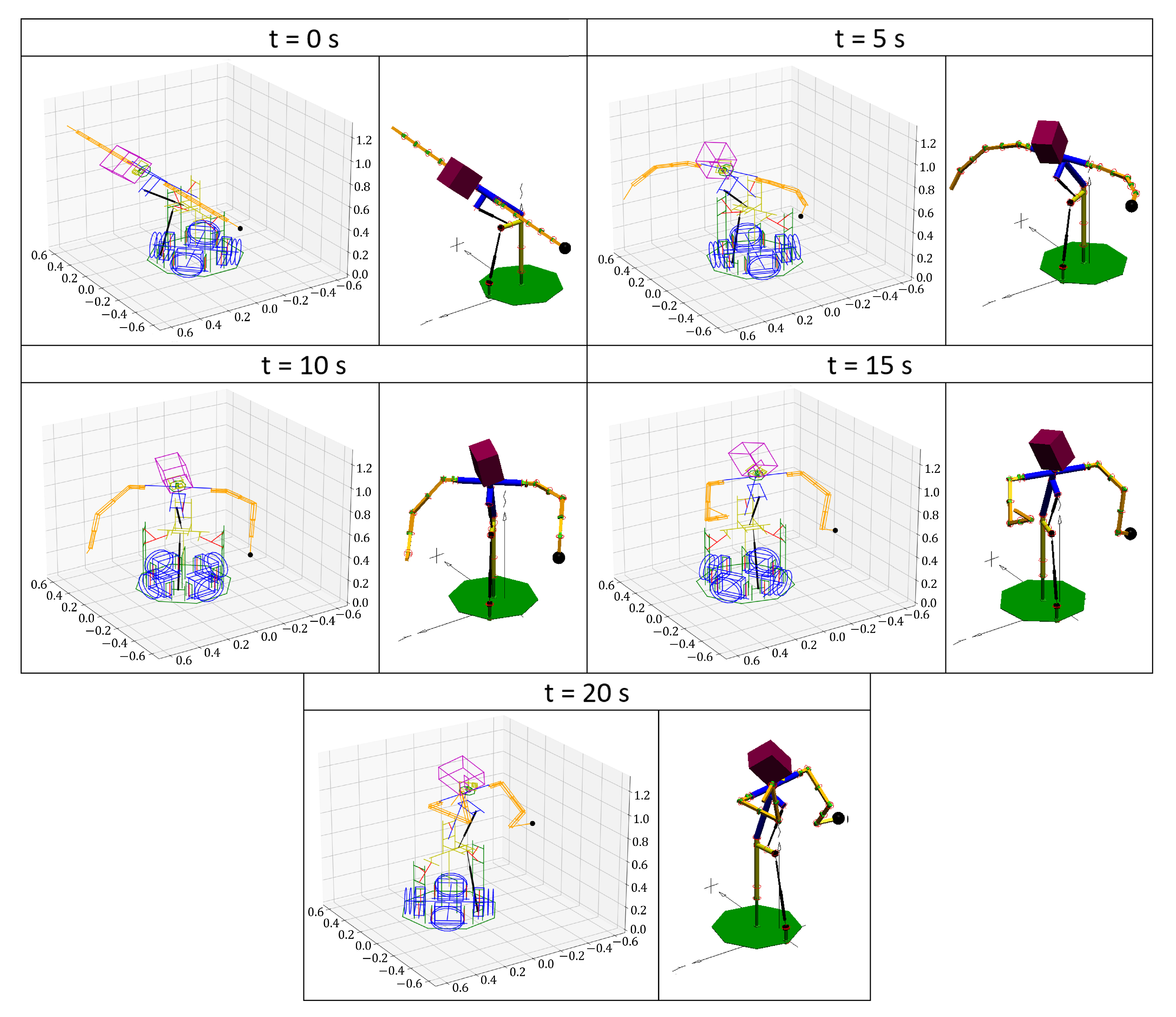
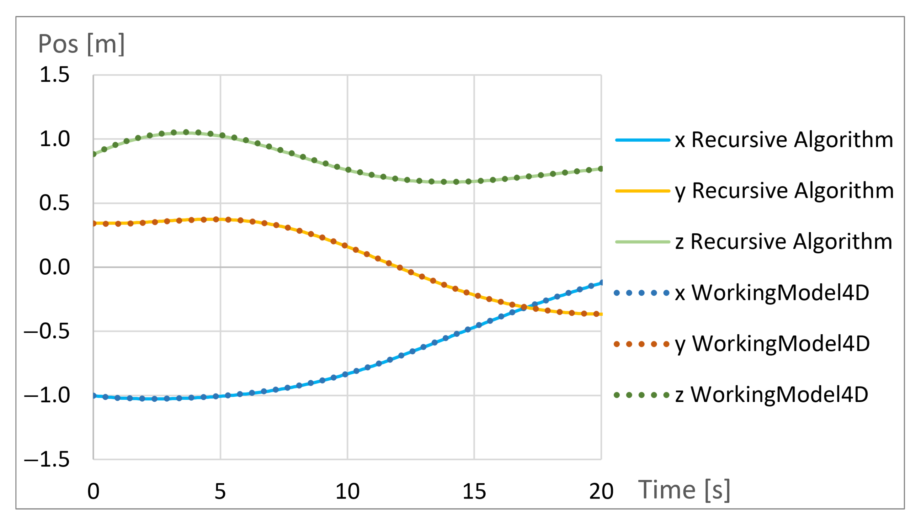
Figure 11 shows a side-by-side comparison of frames captured from both simulation environments, and
Figure 12 compares the extracted coordinates of the center of the left arm end effector (link
).
The figures illustrate that the robot’s behavior was identical in both environments. The results from the extracted data are indistinguishable, with a complete overlap between the graphic’s lines. This data compares positions directly, not orientations (due to the many different notations available to define them), however, similar results for the positions could only be obtained with the correct definition of all the angles in the kinematic chain leading up to link
. The similar configuration of both robots, in
Figure 11, further proves the cohesion between the orientations defined in the two methods.
With these two unrelated sources providing the same results for the robot’s forward kinematics, the validity of the proposed algorithm is proven.
5. Conclusions
In this paper, a simple, intuitive, and theoretically computational efficient three-step recursive algorithm is presented to analyze the kinematics of robotic manipulators. From known joint values, the algorithm fully defines the 3D configuration of a kinematic chain, returning the orientation and position of each link described by rotation matrices and Cartesian coordinates. This methodology was further explained by successfully applying it to model CHARMIE, a mobile manipulator with a relatively high degree of complexity. The results were validated by comparing them with the multibody dynamics software WorkingModel4D.
All input data required to define the given example is provided with full transparency, guaranteeing its replicability. This both exposes the results to external validation and allows the presented problem to serve as a benchmark for 3D kinematic analysis.
After using this methodology, the following key advantages were identified:
Modularity—Due to its recursive structure, models constructed with the proposed algorithm have high modularity. Entire sections in the middle of the kinematic chain can be altered with minimal effort, simplifying any changes made to both links and joints.
Speed of implementation—After the initial equations are defined, this method allows a fast modeling of different kinematics structures. For reference, each of the models shown in
Figure 3 was made in approximately four hours (including the modeling of each link in local coordinates and defining the 3D drawing of the visual interface).
Full definition of the link’s models—The algorithm contains information regarding the geometry of each of the links. This can be used for studies such as collision detection.
Versatility—As previously stated, the implementation of this algorithm is less rigid then the Denavit–Hartenberg parameters, freeing the choice of axes orientation for each of the links. Any rotation and translation can be programmed between each of the links, allowing the definition of any type of joint. More complex mechanisms can be analysed using a process homologous to example (
Section 4.2).
Compatibility—This algorithm outputs: the Cartesian coordinates of each point in each link in local coordinates; the Cartesian coordinates of each point in each link in global coordinates; the orientation between each pair of successive links in the form of rotation matrices; the orientation of each links in relation to the global reference in the form of rotation matrices. This information can be inputted into a set of already defined algorithms, such as the aforementioned example of inverse multibody dynamic analysis [
4].
With the increasing interest in robotics, the presented method can become a powerful tool for computational analysis. It can be used to define a wide array of robots in three dimensions, and the resulting models can act as a starting point for a set of more advanced studies. In the CHARMIE project, this algorithm already functions as the basis for a multibody dynamic analysis environment and will be used for neural network training.
Theory corroborates that this algorithm increases computational efficiency in comparison to using the Denavit–Hartenberg parameters [
2], however, a relevant future study would be running a set of tests to prove and quantify this improvement.


 ,
, 


