A Robot Arm Design Optimization Method by Using a Kinematic Redundancy Resolution Technique

Abstract

Redundancy resolution techniques have been widely used for the control of kinematically redundant robots. In this work, one of the redundancy resolution techniques is employed in the mechanical design optimization of a robot arm. Although the robot arm is non-redundant, the proposed method modifies robot arm kinematics by adding virtual joints to make the robot arm kinematically redundant. In the proposed method, a suitable objective function is selected to optimize the robot arm’s kinematic parameters by enhancing one or more performance indices. Then the robot arm’s end-effector is fixed at critical positions while the redundancy resolution algorithm moves its joints including the virtual joints because of the self-motion of a redundant robot. Hence, the optimum values of the virtual joints are determined, and the design of the robot arm is modified accordingly. An advantage of this method is the visualization of the changes in the manipulator’s structure during the optimization process. In this work, as a case study, a passive robotic arm that is used in a surgical robot system is considered and the task is defined as the determination of the optimum base location and the first link’s length. The results indicate the effectiveness of the proposed method.

1. Introduction

Optimization methods have been employed in a wide range of areas from economical sciences to design processes in engineering applications. All optimization techniques depend on the numerical and/or algorithmic approach. With the improvement and availability of powerful computers, many techniques for optimization studies are presented. Such methods can be listed as genetic algorithms (GA) [1], Ant Colony Optimization (ACO) [2], and Particle Swarm Optimization (PSO) method [3]. These methods are categorized as modern and nontraditional optimization methods. However, optimization techniques have rewards and drawbacks. Various modifications to improve these techniques have been a focus of many studies. The readers are directed to related resources on methods of optimization and comparative studies such as the study in [4] as well as the review study of the seven stochastic optimization methods that are preferred in optimization of industrial designs [5].

All systems that require an optimum design are inherently redundant. In robotics, among the other possible redundancy of components, kinematic redundancy has been an attractive research area since kinematically redundant robot arms may be used to perform additional task/s while performing their main tasks. This is due to the infinite number of solutions received for the inverse kinematics analysis of a redundant robot resulting in an infinite number of configurations of the robot for the same end-effector pose. Consequently, the motions of the links of a robot that are not affecting the motion of the end-effector are named “self-motion” by Nakamura [6]. The algorithms that are developed to regulate the self-motion of the redundant manipulators for a specific aim are called redundancy resolution techniques.

In this study, a design optimization method is formulated specifically for robot manipulators by using Denavit–Hartenberg parameters. The proposed optimization method adopts a redundancy resolution technique for a kinematically non-redundant manipulator. In this new method, an originally non-redundant manipulator is modified to be a redundant manipulator by including virtual joints. Hence, the employment of a redundancy resolution technique is possible for this modified redundant manipulator. The type and location of the added virtual joints are selected by the designer for selectively optimizing the specific parameters of the robot manipulator. The current approach immerses the robot mechanism designer into the optimization process by providing the convergence steps as design parameters continuously change to their optimal values. Hence, the optimization process becomes more intuitive to the robot mechanism designer than the optimization methods involving randomness. This intuitive approach is our motivation in carrying out this study and the main novelty of this work.

The structural optimization process is carried out, considering the design constraints, to validate the applicability of this new technique. Design optimization procedures followed in the design of industrial robot manipulators [7] and the design of haptic devices [8] are utilized in this present work in terms of analyzing the requirements, stating the problem, assigning design constraints, and nominating objective functions. Consequently, performance indices such as manipulability and condition number can be utilized to evaluate kinematic and/or dynamic performances of manipulators [9]. Specifically, in this present work, the objective function that is used in redundancy resolution via null-space optimization is derived by using the modified form of these two indices.

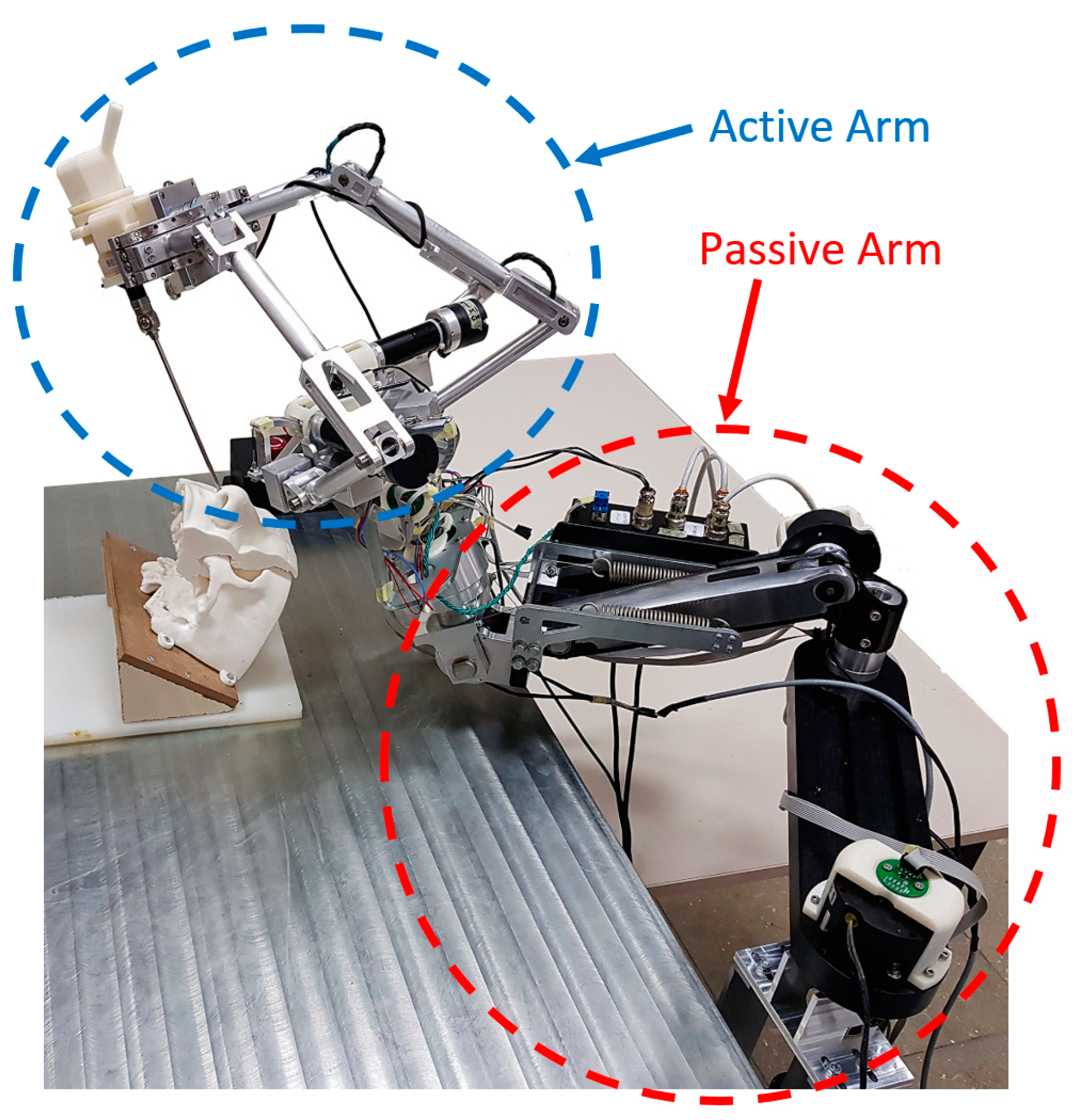
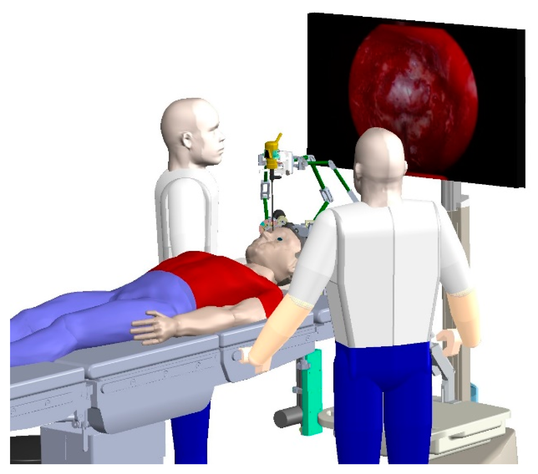
The case scenario selected for this work is the passive arm of a surgical robotic system called NeuRoboScope [10] as shown in Figure 1. In this system, the passive arm is required to be backdriven by the surgeon to the designated locations of the surgical workspace with minimal effort. Therefore, its performance measures related to both kinematic and dynamic manipulability are studied in this paper as objective functions to test the proposed optimization technique. In the next sections, after a brief review of redundancy resolution techniques, the mechanical design optimization technique is described and the passive arm mechanism of the NeuRoboScope system is introduced. Related to this specific case scenario, the design constraints that are used in modifying the problem as the optimization of a two degree-of-freedom (DoF) planar manipulator are explained. This modification also facilitated the understanding and verification of the method described in this paper since the two-DoF planar manipulator is an extensively studied manipulator in the literature. The optimization procedure for this case scenario is explained along with the modifications of the well-known performance indices that are used in this study. Finally, simulations that are carried out to determine the optimal design of the mechanical structure are presented and discussions are given on the obtained results.

2. A Brief Review of Redundancy Resolution Techniques

A variety of redundancy resolution methods have been introduced in the literature such as the Jacobian pseudo-inverse method, weighted pseudo-inverse method, and singularity robustness method (damped least-squares DLS). All those redundancy resolution methods are grouped as Jacobian-based.

By adding constraints in the form of additional tasks to redundancy resolution, the infinite number of solutions is narrowed down to a specific/bounded solution. This is exactly equivalent to establishing design constraints in design optimization techniques. To incorporate an additional task, which is usually called the subtask, to the resolution process of kinematic redundancy, a null-space-based method can be applied. In this method, the gradient of a differentiable objective function is projected in the null-space of the Jacobian matrix so that it does not affect the main task. Here, the main task is the task that is usually assigned as the tracking of the end-effector’s motion trajectory.

Another method of redundancy resolution is the decomposition method which decomposes joint-space variables into two groups (two minor Jacobian matrices) as they are related to the main task and the additional task. Afterward, constraint objective equality is utilized as an implicit function to reduce the gradient of optimization objective function [11]. This method has the attribute of eliminating the unnecessary intensive computation of pseudo-inverse which increases the efficiency of calculation time.

In the task augmentation null-space-based method, the Jacobian matrix is extended by the addition of an auxiliary task [12] to result in a square augmented Jacobian matrix. In this method, the pseudo inverse is not to be used [13] and the kinematic solution is no longer redundant.

Multi-task priority is another null-space-based method [14,15]. In this method, other than the Jacobian matrix related to the main task, for each additional subtask, another Jacobian matrix exists. The self-motion of the first subtask is projected to the null-space of the main task’s Jacobian matrix. The motion of the second subtask is projected into the null-space of the first subtask’s Jacobian matrix. In the same means, other lower-order priority subtasks can be embedded in the earlier subtask that has higher priority.

Among possible secondary tasks, the extra DoFs have been used for obstacle avoidance in [16], mechanical joint-limit avoidance in [17], minimization of joint velocities and accelerations in [18], and reducing interaction forces in physical human-robot interaction in [19]. In [20], the manipulability measure was used, and dynamic manipulability was introduced in [21]. Most methods for resolving redundancy in manipulation involve defining an objective function to satisfy specific additional tasks. In accordance, in the proposed optimization technique presented in this paper, those objective functions are used as potential performance indices to assign design constraints in the optimization problems for structural design of manipulators.

3. Description of the New Mechanical Design Optimization Method for Robot Manipulators

To resolve the redundancy in robot manipulators, first, the manipulator has to be kinematically redundant with respect to the requirements of the task. That is the DoF of the manipulator $n$ should be higher than the DoF needed for the task $m$. In the proposed optimization method, if $n=m$, by including $p$ number of virtual joints, the modified robot arm has $n+p$ DoF and becomes a redundant one. The additional virtual joint variables represent the design parameters of a manipulator. In the structural synthesis of a robot arm, design parameter/s can be any Denavit–Hartenberg (DH) [22] parameter/s shown in Figure 2 other than the joint variable. Hence, (1) for link $k$ that is connected to link $k-1$ via a revolute joint, the possible design parameters are the effective link length $a_k$, the twist angle ${\alpha }_k$ and the relative offset between the two links defined along the revolute joint’s axis of rotation $d_k$ (2) for link $k$ that is connected to link $k-1$ via a prismatic joint, the possible design parameters are the effective link length $a_k$, the twist angle ${\alpha }_k$ and the relative rotation between the two links defined about the prismatic joint’s motion axis passing from the DH joint center ${\theta }_k$. When a virtual joint is included in the manipulator’s mechanism to change the design parameter/s, the self-motion of the robot arm becomes a consequence of the change of the selected design parameter/s.

As a next step, a suitable objective function to be minimized or maximized should be selected to optimize the selected design parameters, which are, in this case, the added virtual joints. The objective functions are generally selected to represent a performance index defined for robot manipulators such as manipulability or condition number. However, the designer can also formulate an objective function based on the requirements of the manipulator’s task.

The aim in this method is to calculate the optimal values of the virtual joints by maximizing or minimizing the objective function via a redundancy resolution algorithm and thus, selecting optimal design parameters. However, for the redundancy resolution algorithm to control the self-motion of the manipulator, joints should move at a finite rate. This means enough time should be provided during the optimization so that the self-motion of the manipulator is completed, and the optimal values of the design parameters are obtained. To ensure that there is enough time for self-motion of the manipulator to be completed, the end-effector of the manipulator is fixed to a specific pose and the convergence of the parameters is observed. This specific pose may be selected as a critical or most visited pose of the manipulator. In this way it is possible to observe the changes in the design parameters as the optimization process is carried out. Consequently, the designer can gain insight into the effect of the design parameters on the performance of the manipulator.

4. Optimization Methodology Described for the Passive Arm of the NeuRoboScope System

In this section, the robot manipulator’s mechanism that is selected as a case study is introduced. Later, the structural synthesis optimization of this robot arm mechanism is explained by defining the specific optimization procedure applied in this case scenario.

4.1. Mechanism of the Robotic Manipulator and the Description of the Case Scenario

The manipulator that is considered for the case scenario is designed as a passive arm of the NeuRoboScope surgical system (Figure 1). The NeuRoboScope system is designated to work alongside the surgeon assisting him/her by handling the camera system, the endoscope, throughout the surgery. The passive arm carries an active arm mounted on its last link and the endoscope is attached to the active arm.

The passive arm has six revolute joints that are not actuated. The surgeon is expected to backdrive the passive arm to locate the active arm at some desired poses during the surgery. Accordingly, the joints of the passive arm are equipped with brake systems to maintain their angular positions when desired by the surgeon.

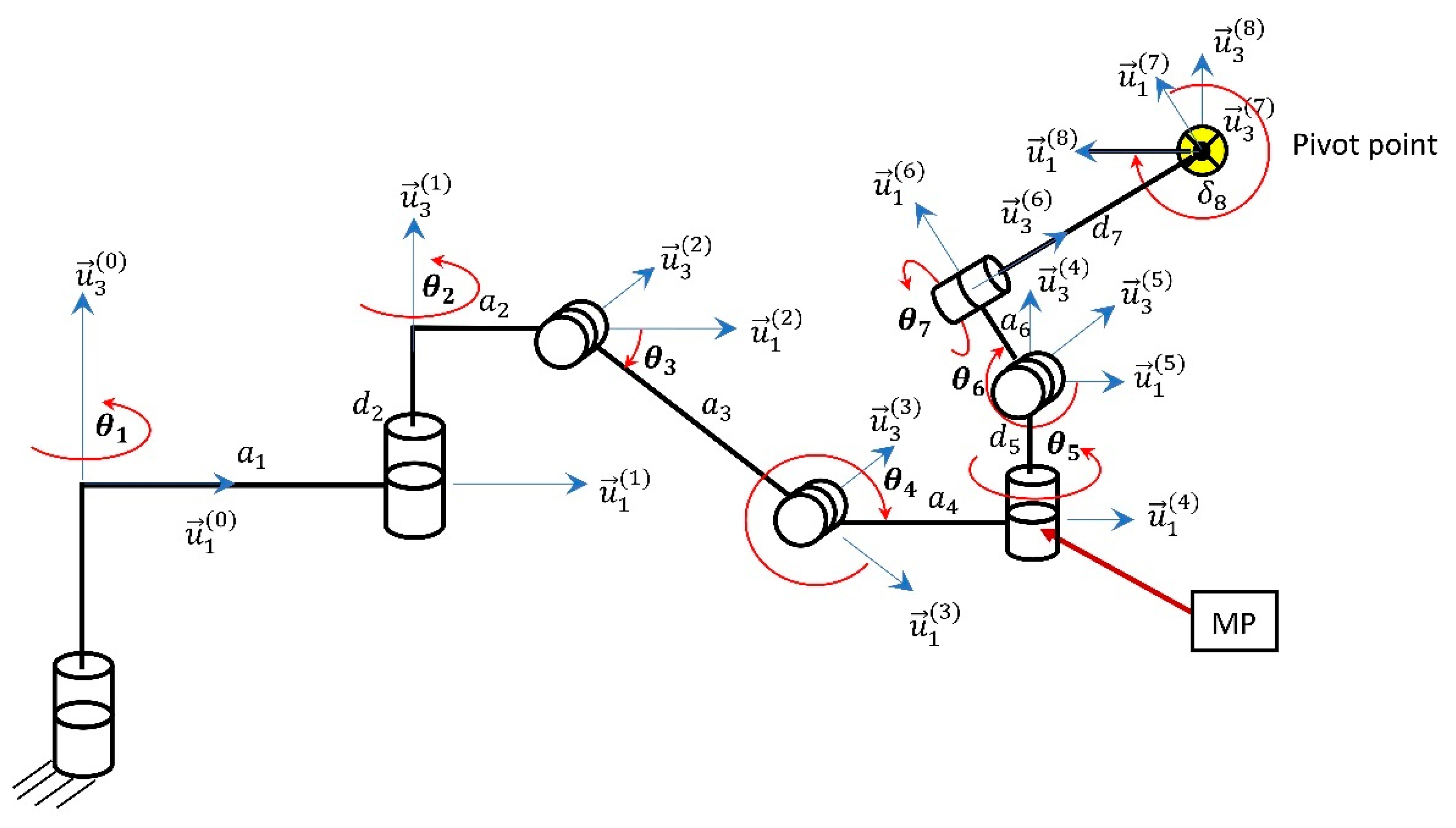
The passive arm’s kinematic architecture is shown in Figure 3. The first two revolute joints are for the planar motion on the horizontal plane. Third and fourth revolute joints have axes parallel to the horizontal plane and they are interrelated to each other with a parallelogram loop so that ${\theta }_3+{\theta }_4=2\pi$. The other three joints compose the wrist mechanism that is responsible for adjusting the orientation of the active arm’s base located at the last link of the passive arm. In Figure 3, MP is identified as the manipulation point at which the ease of manipulation of the passive arm is designated to be calculated.

DH parameters of the passive arm are provided in

Table 1. DH parameters of the passive arm.

$\mathit{k}$	${\mathit{d}}_{\mathit{k}}$	${\mathit{\theta }}_{\mathit{k}}$	${\mathit{a}}_{\mathit{k}}$	${\mathit{\alpha }}_{\mathit{k}}$
1	0	${\theta }_1$	TBD	0
2	$d_2$	${\theta }_2$	$a_2$	$-\pi /2$
3	0	${\theta }_3$	$a_3$	0
4	0	${\theta }_4$	$a_4$	$\pi /2$
5	$d_5$	${\theta }_5$	0	$-\pi /2$
6	0	${\theta }_6$	$a_6$	$-\pi /2$
7	$d_7$	${\theta }_7$	0	$\pi /2$
8	0	${\delta }_8$	0	$-\pi /2$

. In this table, $a_1$ length is kept as to be designed (TBD) on purpose since in the case study, this is the link length that is selected to be optimized for this manipulator. The eighth row of this table indicates the coordinate frame selected for the active arm’s motion definition.

The position of MP is assigned as the maneuvering point which is essential for being a critical consideration for optimization.

$${\overrightarrow{p}}_{MP}=a_1{\overrightarrow{u}}_1^{\left(1\right)}+d_2{\overrightarrow{u}}_3^{\left(1\right)}+a_2{\overrightarrow{u}}_1^{\left(2\right)}+a_3{\overrightarrow{u}}_1^{\left(3\right)}+a_4{\overrightarrow{u}}_1^{\left(4\right)}$$

(1)

In Equation (1), $d_2,a_2,a_3,$ and $a_4$ are assigned as fixed parameters. The only variable is the design parameter that is selected for this optimization study which is the effective link length of the first link, $a_1$.

The joint variables are ${\theta }_1,{\theta }_2,{\theta }_3,$ and ${\theta }_4$, three of which are independent parameters so that the position in the Cartesian space is to be considered as moving on a horizontal plane as related to ${\theta }_1$ and ${\theta }_2$. Apart from that, ${\theta }_3$ is related to the vertical motion and it is selected as a constant value as explained previously. In this way, the passive arm is reduced into a planar revolute-revolute (RR) manipulator. Consequently, the length of the new second link is calculated as $a_2^{*}=a_2+a_4+a_3\cos {\theta }_3$.

The position of the MP is assigned as a constraint for design. Concerning that this position on the horizontal plane and the base of the passive arm is fixed at a specific point on the surgery table, two possible configurations can be calculated as elbow-up and elbow-down. Any one of the two solutions can be selected to find the initial position for each of ${\theta }_1$ and ${\theta }_2$ during the optimization study. The inverse kinematics solutions are not presented here since it is trivial for a planar two DoF revolute-jointed arm.

For verifying and testing the objective function on the actual passive arm, the original Jacobian matrix is a $\widehat{J}\in {\Re }^{2\times 2}$ matrix for the planar arm with two DoF. However, for optimization study, virtual joints are added to the original passive arm and the Jacobian matrix is modified as ${\widehat{J}}_{2\times 4}\in {\Re }^{2\times 4}$ and ${\widehat{J}}_{2\times 3}\in {\Re }^{2\times 3}$. The case with the two virtual joints (${\widehat{J}}_{2\times 4}$) includes a prismatic joint acting along the y-axis and its positive direction motion is defined along $-{\overrightarrow{u}}_2^{\left(0\right)}$ axis by a virtual joint parameter $Y_0$. The other virtual joint in the two-virtual joint case (${\widehat{J}}_{2\times 4}$) and the single-virtual joint case (${\widehat{J}}_{2\times 3}$) is the prismatic joint included to change the effective link length, $a_1$. The dimension of the Jacobian matrix is related to the DoF of the workspace and DoF of the original or modified passive arm. In Equations (2)–(4), Jacobian matrices with two virtual joints, one virtual joint, and no virtual joints are presented, respectively.

$${\widehat{J}}_{2\times 4}=\left[\begin{array}{cccc}0& c1& -a_{1}s1-\left(a_2+a_4+a_{3}c3\right)s12& -\left(a_2+a_4+a_{3}c3\right)s12\\ -1& s1& a_{1}c1+\left(a_2+a_4+a_{3}c3\right)c12& \left(a_2+a_4+a_{3}c3\right)c12\end{array}\right]$$

(2)

$${\widehat{J}}_{2\times 3}=\left[\begin{array}{ccc}c1& -a_{1}s1-\left(a_2+a_4+a_{3}c3\right)s12& -\left(a_2+a_4+a_{3}c3\right)s12\\ s1& a_{1}c1+\left(a_2+a_4+a_{3}c3\right)c12& \left(a_2+a_4+a_{3}c3\right)c12\end{array}\right]$$

(3)

$${\widehat{J}}_{2\times 2}=\left[\begin{array}{cc}-a_{1}s1-\left(a_2+a_4+a_{3}c3\right)s12& -\left(a_2+a_4+a_{3}c3\right)s12\\ a_{1}c1+\left(a_2+a_4+a_{3}c3\right)c12& \left(a_2+a_4+a_{3}c3\right)c12\end{array}\right]$$

(4)

In the equations above, $sk=\sin {\theta }_k$ and $ck=\cos {\theta }_k$ for $k=1,2,3$, and $s12=\sin \left({\theta }_1+{\theta }_2\right)$ and $c12=\cos \left({\theta }_1+{\theta }_2\right)$.

4.2. Design Optimization Constraints

NeuRoboScope system is designed to be used in a minimally invasive pituitary tumor surgery. In this surgery, the natural openings through the nostrils are used to insert surgical tools. Hence, the passive arm of NeuRoboScope system is back-driven manually by the surgeon while the surgeon places the endoscope in and out of the nostril. Concerning this special use of the passive arm, design constraints are defined below.

• The surgeon can insert the endoscope from either nostril.
• The endoscope and the active robot arm should not interfere with the surgeon’s hands, and they should not block the surgeon’s view of the monitor, see Figure 4.
• The passive arm should locate the active arm inside the surgery workspace by approaching from behind the patient’s head.
• The passive arm should be fixed to the surgery table.
• Physical dimensions of the links should not be large, and they should not be heavy, but they should be rigid enough to compose an inertial frame for the active arm when their brakes at the joints of the passive arm are activated.
• There should be no actuators on the joints of the passive robot arm.
• When the passive arm’s brakes are released, the surgeon should be able to move the endoscope freely while the endoscope is still attached to the active robot arm.

A study can be carried out for all of the DH parameters, excluding the joint variables, of the passive arm. However, in this study, the passive arm’s motion on the horizontal plane is considered to facilitate the demonstration of the optimization method. Accordingly, from this point on, the kinematics of the passive arm are reduced to a 2-DoF planar robot arm with two revolute joints. Design parameters that are considered are the effective link length of the first link and the ground frame’s origin, which is the location that the passive arm is fixed on the surgery table.

4.3. Optimization through Mechanical Redundancy

Depending on the previously defined design constraints, the requirements for the passive arm are set for the optimization procedure by considering the necessities and conditions of the surgery:

• The surgeon should have minimal effort when he/she intends to push the active robot arm in or away from the surgery zone.
• The parallelogram loop in the passive robot arm is utilized with no modifications since it is designed with counter-spring for gravity compensation. This linkage is responsible for providing vertical motion of the base of the active arm.
• The optimization is related only to the ease of manipulation only on the horizontal plane.
• The fixing point position on the y-axis (with respect to reference-frame in Figure 5) is selected as a possible design parameter, which is related to another design parameter that is the first link’s length.
• MP position is fixed at the coordinate (−20, −30) cm (which can be considered as an average position of workspace required by the surgeon) relative to the reference frame in Figure 5.
• The effective link length of the first link should be limited depending on its manufacturability, final weight and allowed compliant displacements due to loads.
• The linear density of the first link is taken as follows: mass/length = 1 kg/m.
• The third joint variable ${\theta }_3$ in Figure 3 is fixed at −30° which is the condition when the endoscope is located just above the patient’s nostrils.

Since the objective of the optimization is to ease the manipulation at MP, which is denoted in Figure 3, forward and inverse kinematics, and the Jacobian matrix calculations are presented for MP. Hence, these calculations are used for the proposed optimization method.

5. Implementation of the New Optimization Strategy

When there is kinematic redundancy, there is a free motion of the mechanism even if the end-effector is fixed. This so-called self-motion happens in the null space of the Jacobian matrix. In the implementation of the proposed optimization strategy, this property is used. However, to use this property, the non-redundant passive arm must be modified to have more joints.

For the case with two virtual joints, the DoF of the RR planar arm is increased by 2. Consequently, a 4-DoF PRPR planar arm operating for a 2-DoF planar task is formed. Since the objective is to find optimum design parameters, these new joint variables ($Y_0$ and $a_1$) are included in the control of the self-motion of the resultant redundant arm.

Although a designer is free to choose any redundant manipulator controller, a previously designed controller for redundant robot manipulators is utilized for this optimization task [18]. However, only the kinematic part of this controller is used in this work. This controller is used to control both the main task in task-space, earlier defined by the MP point’s position $\overline{x}$ in horizontal plane, and a desired subtask by adjusting the joints’ motion in the null space.

An error term is defined as $\overline{e}={\overline{x}}_d-\overline{x}$ as the tracking error, and ${\overline{x}}_d$ is defined as the desired position/trajectory in task-space. The designed controller is presented in Equation (5) where ${\widehat{K}}_v$ and ${\widehat{K}}_p$ are diagonal constant feedback gain matrices related to the proportional-derivative (PD) controller of the main task.

$$\ddot{\overline{q}}={\widehat{J}}^{+}\left({\ddot{\overline{x}}}_d+{\widehat{K}}_v\dot{\overline{e}}+{\widehat{K}}_p\overline{e}-\dot{\widehat{J}}\dot{\overline{q}}\right)+{\ddot{\overline{\beta }}}_N$$

(5)

The column of joint variables in position level are denoted as $\overline{q}$ $\in {\Re }^n$, where $n$, from now on, is the summation of actual and virtual joints in this approach. We consider that a vector function $\overline{z}(.)\in {\Re }^n$ is calculated as a gradient of optimization objective function $f\left(\overline{q}\right)$ for a specific optimization objective function (which may be time-dependent function, including design constraints, etc.), and joint velocities in the null space are required to track the projection of $\overline{z}$ onto the null space of $\widehat{J}$. Since ${\widehat{I}}_n-{\widehat{J}}^{+}\widehat{J}$ projects vectors onto the null space of $\widehat{J}$, this can be formulated in an error signal calculation as presented in Equation (6), which converges to zero. Here, ${\widehat{J}}^{+}$ represents the pseudo-inverse of $\widehat{J}$ and ${\widehat{I}}_n$ $\in {\Re }^{n\times n}$ is the identity matrix.

$${\dot{\overline{e}}}_N=\left({\widehat{I}}_n-{\widehat{J}}^{+}\widehat{J}\right)\overline{z}-{\dot{\overline{\beta }}}_N$$

(6)

Assuming the manipulator does not go through a singularity condition, it is needed to design ${\ddot{\overline{\beta }}}_N$ to obtain the desired result for the subtask objective. ${\ddot{\overline{\beta }}}_N$ is determined as;

$${\ddot{\overline{\beta }}}_N=\left({\widehat{I}}_n-{\widehat{J}}^{+}\widehat{J}\right)\dot{\overline{z}}-\left({\widehat{J}}^{+}\dot{\widehat{J}}{\widehat{J}}^{+}+{\widehat{J}}^{+}\right)\widehat{J}\overline{z}+{\widehat{K}}_N{\dot{\overline{e}}}_N$$

(7)

In Equation (7), ${\widehat{K}}_N$ is a diagonal positive definite feedback matrix. This designed control law guarantees that the error will be bounded and converged to zero [18]. After the description of the controller to be used in the proposed optimization method, the performance indices that are used to formulate the objective function are explained in the next subsections. It should be noted that instead of the performance metrics mentioned below, the objective function can be developed by considering other performance metrics and/or their variations.

5.1. Manipulability Ellipsoid and Singular Value Decomposition (SVD)

Manipulability of a selected point in a mechanical linkage can be represented as a scalar value related to the area/volume of velocity ellipse/ellipsoid calculated at this point. It is first developed in [20] and introduced as a performance index. Since the motion of any point on a mechanical linkage can be related to the motion of the joints by the Jacobian matrix, the scalar representation of the manipulability index $Mp$ is provided in the following equation.

$$Mp=\sqrt{det(\widehat{J}{\widehat{J}}^T)}$$

(8)

In addition to the manipulability index shown in Equation (8), another manipulability measure in Equation (9) was also formulated by Paul and Stevenson [23] as follows

$$Mp=|det(\widehat{J})|.$$

(9)

The objective set when using the manipulability index is to maximize this value via changing the positions of joints by staying inside the null-space when MP is fixed at the desired position. During this motion, the effective link length of the first link ($a_1$) and the position of the fixing point of the passive arm ($Y_0$) will be changing to reach the optimum value in this optimization.

Singular value decomposition on the matrix $\widehat{J}{\widehat{J}}^T$ is used to solve for singular values of $\widehat{J}$, which also represents the semi-axes of manipulability ellipse during the simulation. The rank of $\widehat{J}$ represents the number of singular values, which is two in this case because in the formulation of the objective function, the Jacobian matrix is related to the original manipulator.

5.2. The Modified Condition Number

Another way to represent force/motion relation of a point in the workspace of a mechanism is done by a scalar number called condition number [24]. Manipulability represents ease of manipulation of the end-effector at a certain location of the workspace and the condition number relates the length of the maximum and minimum axes of manipulability ellipse achieved along with different directions at that specific location of the end-effector. The condition number is represented by the ratio of the maximum singular value to the minimum singular value of the Jacobian matrix, which represents the radii of the manipulability ellipse. The distance between any point on the ellipse and its center was defined in [25] as the velocity transmission ratio on one specific direction of motion of the end-effector. In an ideal case, the performance index is 1, which means at that specific point, the velocity transmission ratio is the same in all directions and a circle will be representing the manipulability.

Force condition number and velocity condition number are calculated in similar ways. Salisbury and Craig [24] introduced force condition number as the amplification of the relative force error at the task-space to the relative torque error at the joint-space. While Merlet [26] described a velocity condition number using relative motion error in joint-space and relative motion error in the task-space.

In this work, the difference between the maximum and minimum singular values of the Jacobian matrix (${\sigma }_{max}$ and ${\sigma }_{min}$, respectively) is used instead of the condition number and it will be referred as the modified condition number from this point on. The objective function shown in Equation (10) is used in the optimization procedure to be minimized to a minimum value or if possible zero value.

$$C_n={\sigma }_{max}-{\sigma }_{min}$$

(10)

5.3. Generalized Inertia Matrix

To include a dynamic orientated design constraint for the design of the passive arm, the dynamic model of the arm is studied via finding its dynamic equation of motion and the generalized inertia matrix. This is essential to find the dominant part of design parameters in the relation between the forces displayed at the end-effector and the consequent motion of the manipulator. In this work, since the end-effector is moved at a slow rate, Coriolis and centripetal forces, and the viscous frictional forces are neglected. Consequently, the remaining part of the dynamic equation is shown below.

$$\overline{\tau }=\widehat{M}\ddot{\overline{q}}$$

(11)

In Equation (11), $\overline{\tau }$ is the column of actuator torques/forces acting on the joints and $\widehat{M}$ is the generalized inertia matrix. To represent Equation (11) in the task-space, where the interaction is taking place, the task-space forces are mapped to the joint space forces by using the Jacobian matrix as follows:

$$\overline{\tau }={\widehat{J}}^T\overline{F}.$$

(12)

Here, in Equation (12), $\overline{F}$ is the external forces acting at the end-effector. For the slow-motion of the end-effector, where $\dot{\overline{q}}\to 0$, we consider $\ddot{\overline{q}}={\widehat{J}}^{-1}\ddot{\overline{x}}$. Subsequently,

$${\widehat{J}}^T\overline{F}=\widehat{M}{\widehat{J}}^{-1}\ddot{\overline{x}}.$$

(13)

As a result of this expression in Equation (13), mapped generalized inertia matrix ($mGIM$) ${\widehat{M}}_G$ is defined in the task-space as shown in Equation (14).

$${\widehat{J}}^{-T}\widehat{M}{\widehat{J}}^{-1}={\widehat{M}}_G$$

(14)

The dynamic performance of the passive arm can be represented by the ellipse (in the case of the 2-DoF manipulator) which can be plotted for the eigenvalues and eigenvectors of ${\widehat{M}}_G$ matrix [27]. On the other hand, the dynamic manipulability (the determinant of $\widehat{J}{\widehat{M}}^{-1}$) as defined in [21] by Yoshikawa relates the loads at actuators to the acceleration output at end-effector as shown in Equation (15).

$$\ddot{\overline{x}}=\widehat{J}{\widehat{M}}^{-1}\overline{\tau }$$

(15)

For the design optimization study of the passive arm, the objective is to minimize the resistance shown to the operator during he/she backdrives the arm, which can be termed as the mechanical impedance [28] of the passive arm. By doing so, the end-effector can be moved freely inside its workspace with minimum force reflected to the user. This can be achieved by either minimizing the determinant of the numerator part of ${\widehat{M}}_G$ in Equation (14) hence the generalized inertia matrix ImN (previously defined as $\widehat{M}$), and/or maximizing the determinant of denominator part of ${\widehat{M}}_G$, which corresponds to the manipulability index $\mathit{ImD}$ since $\det ({\widehat{J}}^T\widehat{J})=\det (\widehat{J}{\widehat{J}}^T)$. In this work, the mapped generalized inertia matrix ${\widehat{M}}_G$ and its abovementioned numerator ($\mathit{ImN}$) and denominator parts ($\mathit{ImD}$) are used as indicators of the dynamic performance measure while selecting the objective function.

6. Simulation Tests and Results

Two simulation tests are conducted to verify the presented approach. Two design parameters are used for both tests. The Jacobian matrix developed for the MP of the actual passive arm (RR manipulator version) is used to determine the desired objective function that is related to the modified condition number. All tests are carried out in Matlab Simulink setting the fixed step calculation frequency to 100 Hz with an ODE3 solver. The fixed position of MP is selected as a design constraint on the horizontal planar workspace at −20, −30 cm for this particular scenario of the presented case study, which is determined relative to the frame described in Figure 5. In all the tests, the initial value of the first link is chosen as $a_1=30$ cm and the initial value of fixing position (first joint’s axis location) along the y-axis is selected to be $Y_0=0$ cm. The other parameters of the passive arm are assigned as fixed parameters.

6.1. Simulation Test with the Modified Condition Number Performance Index

In this test, the modified condition number and the manipulability index is calculated to visualize the effect of the optimization. Both the fixing point of the manipulator along the y-axis and the first link’s length are selected as design parameters.

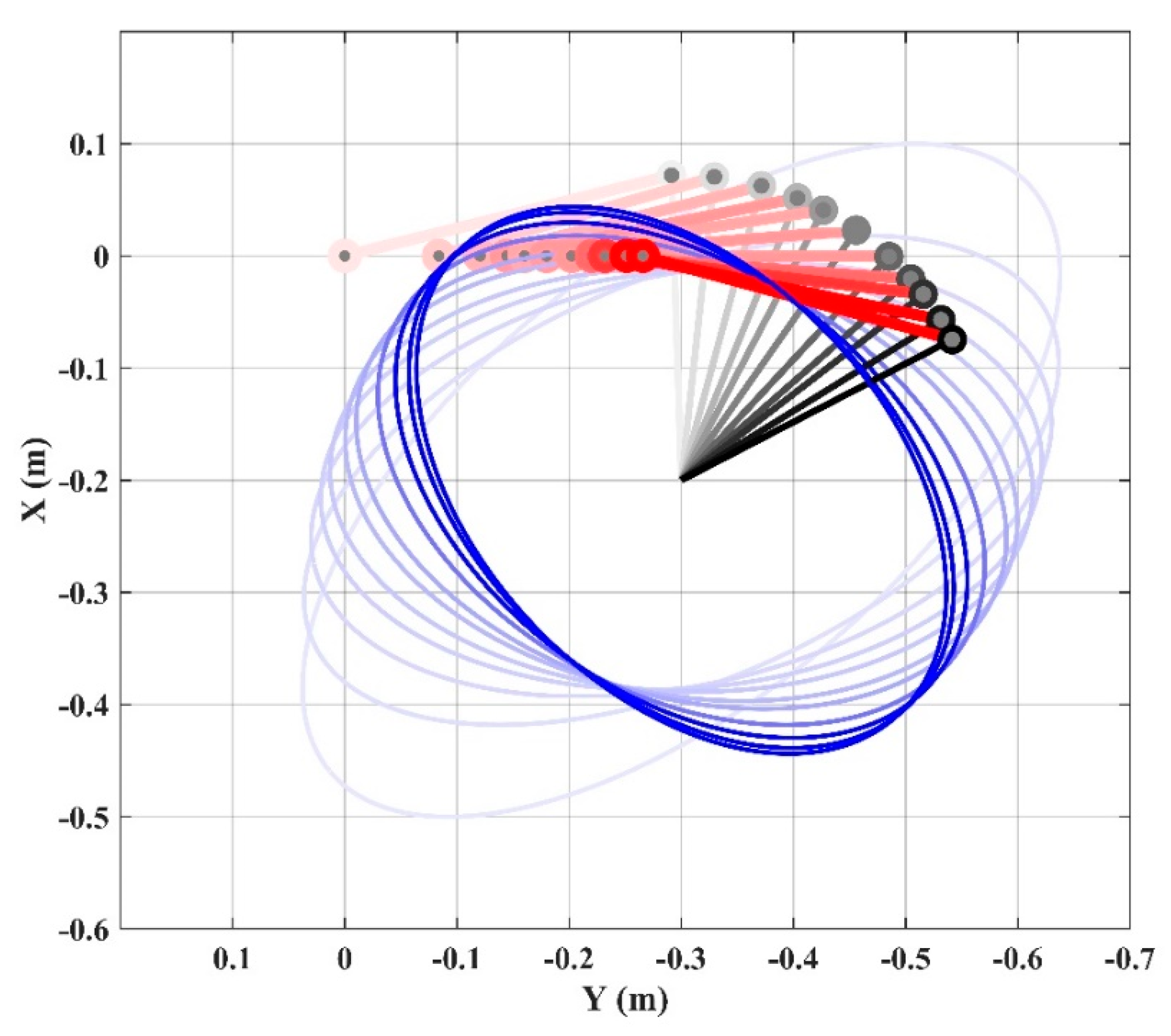
By using the modified condition number, which is presented in Equation (10), as the only performance index in forming the objective function $f\left(\overline{q}\right)=-Cn$, singular values are forced to be equal during the optimization procedure due to the minimization of the objective function. As a result, the manipulability ellipse is forced to be a circle and the robot arm moves into an isotropic pose as can be seen in Figure 6.

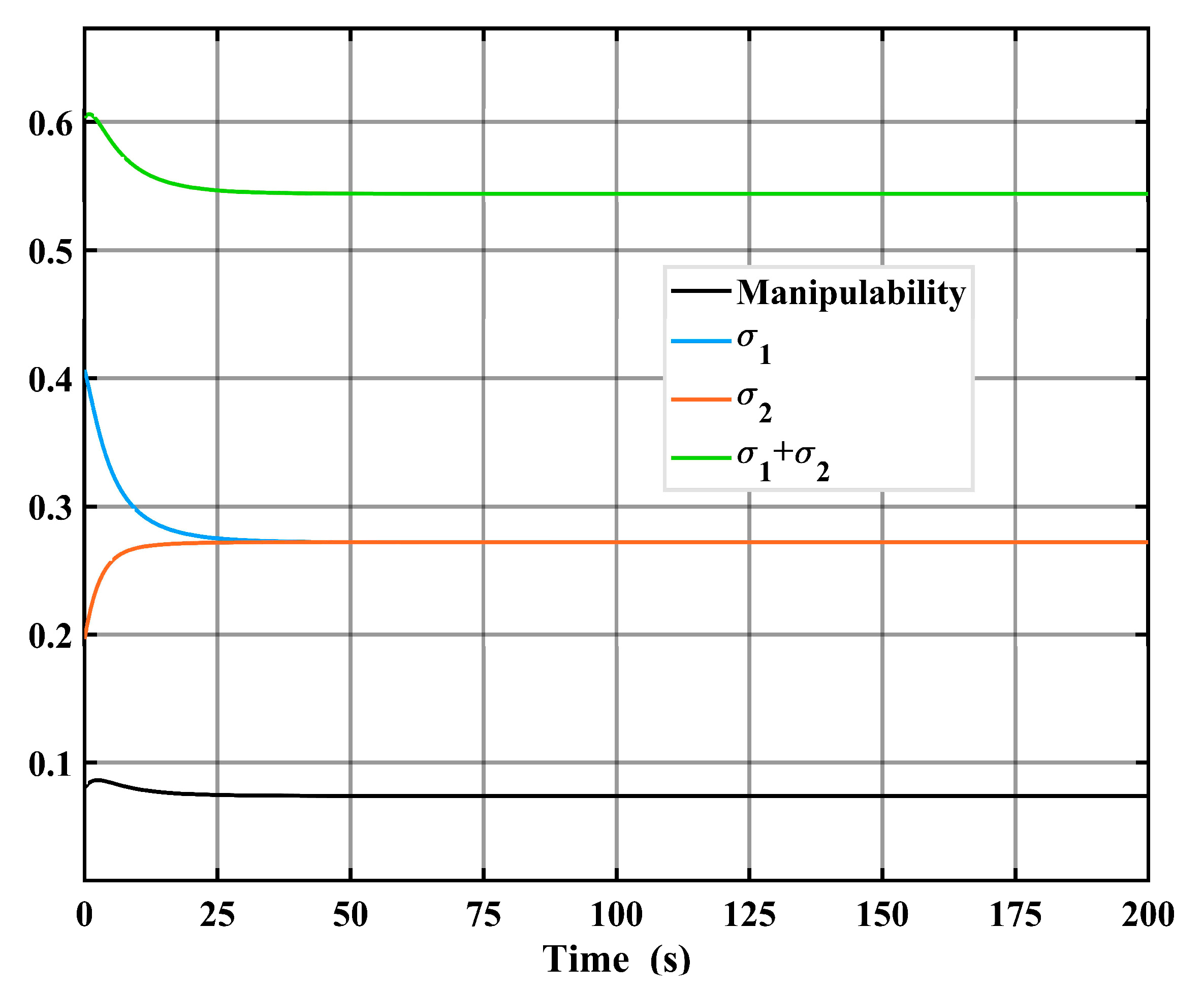
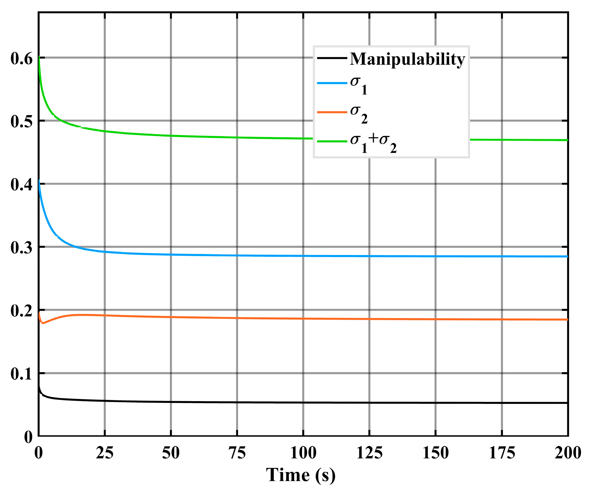
This result is the same result that is presented and discussed in [29]. The obtained results are exactly as expected for the isotropic pose. The optimal length of the first link came out to be $a_1=38.47$ cm which is equal to $a_1=a_2\sqrt{2}$. The fixing point position converged to a position at $Y_0=-11.57$ cm. It is observed in Figure 7 that the manipulability index decreases while the modified condition number index increases which is making maximum and minimum singular values to be equal.

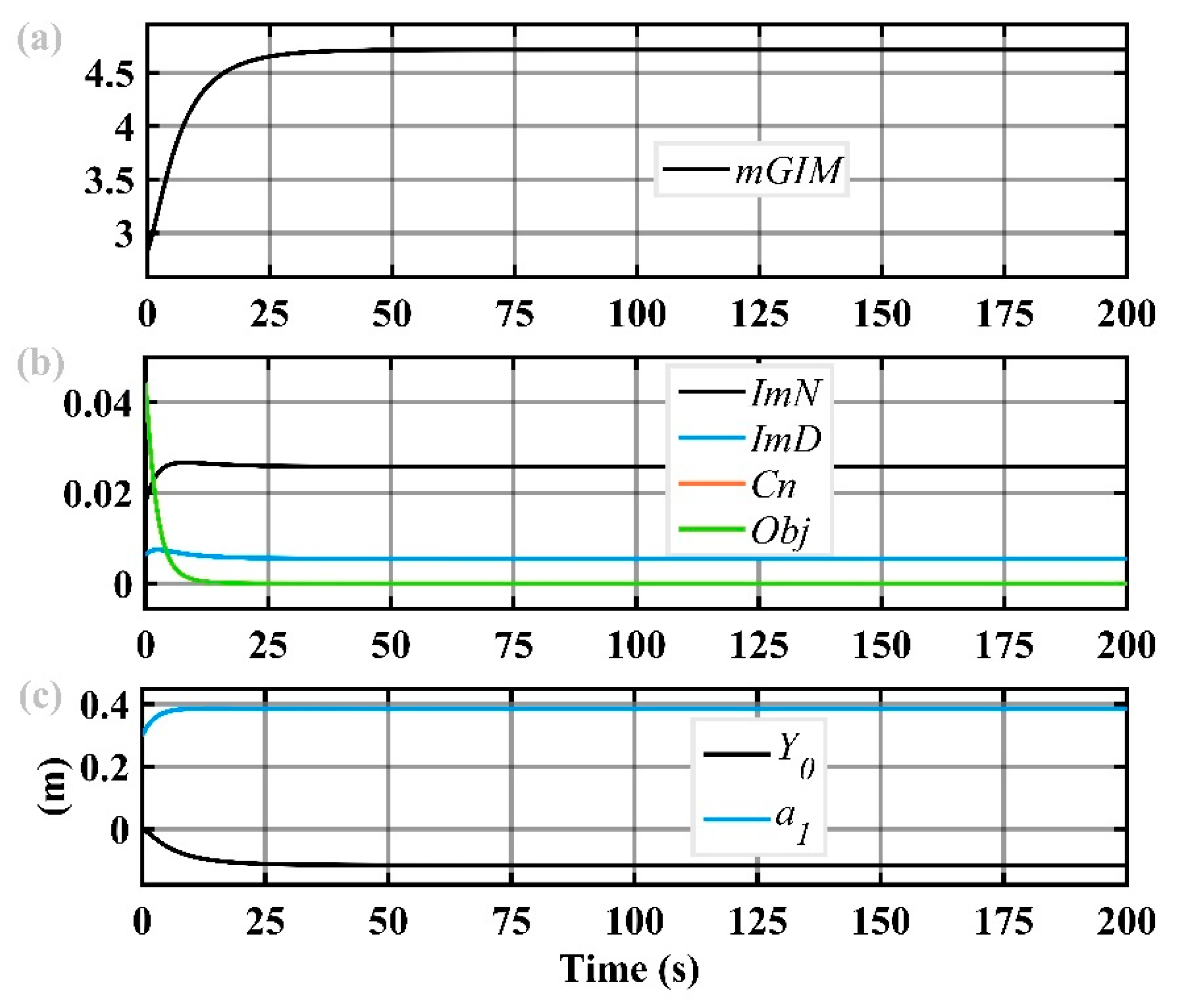
As another consideration of the optimization process, the variation of inertial properties of the manipulator is investigated. In Figure 8a, it can be noticed that the determinant of the mapped generalized inertia matrix (mGIM) is increased because of this optimization. This is due to the increase in the first link length and decrease in overall manipulability. In addition, the determinant of the generalized inertia matrix (the numerator of mGIM) is increased as can be seen in Figure 8b, which is represented by $\mathit{ImN}$ in this figure. $\mathit{ImD}$ represents manipulability (the denominator of mGIM). As the objective function is minimized, the modified condition number becomes zero since in this work, it is described as the difference between the maximum and minimum singular value of the manipulability matrix.

During the optimization process, design parameters could converge to constant values. As shown in Figure 8c, the length of the first link is increased due to this optimization, which leads to a decrease in manipulability and as a result increase in the determinant of $mGIM$. This can be considered as a drawback but the objective in using the modified condition number is to result in an isotropic pose in terms of manipulability index.

6.2. Simulation Test with the Modified Condition Number Performance Index and Generalized Inertia Matrix

In this final test, modified condition number and the numerator part of the mapped generalized inertia matrix, which corresponds to the generalized inertia matrix, are used with selected weights of $w_1=1$ and $w_2=2$ in forming the objective function, respectively. In this way, the objective function is modified to have both the effect of modified condition number and the determinant of the generalized inertia matrix $ImN$ as $f\left(\overline{q}\right)=-w_1{C}_n-w_{2}ImN$. As a result, shorter length for the first link is obtained and manipulability ellipse is reshaped as can be noticed in Figure 9. In Figure 6 and Figure 9: (1) the red line indicates the first link, and the black line indicates the second link, (2) the joint centers for the first and second joint are indicated with red and black circles, respectively (3) during the optimization process, the link colors are drawn darker as the links move from their initial states to their final states.

In this optimization procedure, due to the decrease in manipulability, which is shown in Figure 10, and the decrease in the determinant of generalized inertia matrix $ImN$, which is shown in Figure 11b, the determinant of $mGIM$, as shown in Figure 11a, is increased more relative to the results presented in Section 6.1. The positive result of this optimization is obtaining a smaller link length for the first link, which is indicated in Figure 11c. Nevertheless, the weights used for the influence of the modified condition number and the inertia matrix on the objective function is critical. The choice of these weights could decrease manipulability in one direction to a value near zero, which would minimize the backdrivability of the manipulator in that direction.

7. Validation of the Proposed Optimum Design Approach

To ease the comparison of our optimization approach, we named our optimization approach as Optimization via Redundancy Resolution (ORR). To show the accuracy of the proposed optimization approach, we compared the results obtained by stochastic optimization algorithms Simulated Annealing (SA) algorithm, Differential Evolution (DE) algorithm, Nelder–Mead (NM) algorithm, Random Search (RS) algorithm, based on four different phenomenological search approaches, and that of ORR for the mechanism design problem we defined. Here, the basic rationale for choosing these algorithms for validation is (i) they have proven their reliability in the solution of mathematical optimization problems, which have been used in many different disciplines, (ii) because they have different phenomenological bases, a solution alternative that an algorithm might miss can be compensated by this way. At this stage, two different optimization scenarios were defined: First, to find the results that minimize only the $C_n$ parameter, and in this context, optimize the parameters $Y_0$, ${\theta }_1$, ${\theta }_2$ and $a_1$ under the given nonlinear equality and linear inequality constraints; The second was to define the importance levels of the $C_n$ and $ImN$ parameters with the weight values of $w_1$ and $w_2$, to define a new objective function ($w_1{C}_n+w_{2}ImN$) and to use the constraints used in the first scenario. Weights are selected as $w_1=1$ and $w_2=2$ in forming the objective function, respectively. The unit for the distances is $\mathrm{m}$ and the unit for the angular positions is rad in description of the two optimization scenarios.

Find design variables: $Y_0$, ${\theta }_1$, ${\theta }_2$, $a_1$

Scenario 1:

To minimize the objective function: $C_n\left(Y_0, {\theta }_1, {\theta }_2, a_1\right)$

Scenario 2:

To minimize the objective function: $w_1{C}_n\left(Y_0, {\theta }_1, {\theta }_2, a_1\right)+w_{2}ImN\left(Y_0, {\theta }_1, {\theta }_2, a_1\right)$

Subjected to: $-1\le Y_0\le 0,0<a_1<0.5$

$a_2=0.350;$

$a_3=0.216;$

$a_4=0.05;$

${\theta }_3=-30\pi /180;$

$X_0=0;$

$a_2^{*}=a_2+a_4+a_3\cos {\theta }_3;$

$\left[X_{MP},Y_{MP}\left]=\right[-0.2,-0.3\right]$

$X_{MP}=a_1\cos \left({\theta }_1\right)+a_2^{*}\cos \left({\theta }_1+{\theta }_2\right);$

$Y_{MP}=Y_0+a_1\sin \left({\theta }_1\right)+a_2^{*}\sin \left({\theta }_1+{\theta }_2\right);$

where

$$\begin{array}{ll}{C}_n\left(Y_0,{\theta }_1,{\theta }_2,a_1\right)& =\frac{1}{2}\left(\right((a_1^2+{\left(a_1^4+1.088a_1^3\cos \left({\theta }_2\right)+0.592a_1^2{\cos }^2\left({\theta }_2\right)+0.161a_1\cos \left({\theta }_2\right)+0.022\right)}^{0.5}\\ & +0.544a_1\cos \left({\theta }_2\right)+0.148)\\ & -{\left(\right(a_1^2-(a_1^4+1.088a_1^3\cos \left({\theta }_2\right)+0.592a_1^2{\cos }^2\left({\theta }_2\right)+0.161a_1\cos \left({\theta }_2\right)+0.022}^{0.5})\\ & {{{+0.544a_1\cos \left({\theta }_2\right)+0.148)}^{0.5})}^{0.5})}^2\end{array}$$

$$ImN\left(Y_0, {\theta }_1, {\theta }_2, a_1\right)=0.172707a_1^2+0.100746a_1^3-0.0740175a_1^2{\cos }^2\left({\theta }_2\right)$$

In the Appendix A, summary information about the working logic of the optimization algorithms we use for validation is given. For more detailed information, you can refer to the relevant reference [5].

For the optimization problems solved for the scenarios, the algorithm options given in

Table 2. Corresponding options for the optimization algorithms DE, NM, RS, and SA.

Options	DE	NM	RS	SA
Crossover fractions	0.5	-	-	-
Random Seed	1	5/10	0	2
Scaling factor	0.6	-	-	-
Tolerance	0.001	0.001	0.001	0.001
Contact ratio	-	0.5	-	-
Expand ratio	-	2.0	-	-
Reflect ratio	-	1.0	-	-
Shrink ratio	-	0.5	-	-
Level iterations	-	-	-	50
Perturbation scale	-	-	-	1.0
Penalty Function	-	-	Automatic	-
Search Points	-	-	2	-
Method	-	-	Interior Point	-

are used.

The obtained results using the four well-established optimization algorithm’s results are tabulated along with the result obtained by the proposed ORR algorithm. Due to the “RandomSeed” dependency, which is one of the advantages of the NM algorithm, it is possible to produce alternative results when two different choices (5 and 10) are made for this problem. Therefore, the results for two version of NM are also presented.

Table 3. The optimization results for Scenario 1 obtained via DE, NM, RS, SA and ORR algorithms.

Optimization Algorithm	Objective Function	${\mathit{Y}}_0\left(\mathbf{cm}\right)$	${\mathit{\theta }}_1\left(\mathbf{rad}\right)$	${\mathit{\theta }}_2\left(\mathbf{rad}\right)$	${\mathit{a}}_1\left(\mathbf{cm}\right)$
SA	2.21008 × 10−14	−11.56	−1.611	−2.356	38.48
DE	1.21496 × 10−13	−11.56	3.079	2.356	38.48
NM1	8.39033 × 10−15	−48.44	1.611	2.356	38.48
NM2	2.21008 × 10−14	−11.56	−1.611	−2.356	38.48
RS	2.21008 × 10−14	−11.56	−1.611	−2.356	38.48
ORR	5.03038 × 10−9	−11.57	−1.611	−2.356	38.47

and

Table 4. The optimization results for Scenario 2 obtained via DE, NM, RS, SA and ORR algorithms.

Optimization Algorithm	Objective Function	${\mathit{Y}}_0\left(\mathbf{cm}\right)$	${\mathit{\theta }}_1\left(\mathbf{rad}\right)$	${\mathit{\theta }}_2\left(\mathbf{rad}\right)$	${\mathit{a}}_1\left(\mathbf{cm}\right)$
SA	0.0363314	−30.00	−1.998	−2.408	28.50
DE	0.0363314	−30.00	1.998	2.408	28.50
NM1	0.0363314	−29.997	−1.998	−2.408	28.49
NM2	0.0363314	−29.994	1.998	2.408	28.50
RS	0.0363314	−30.00	1.998	2.408	28.50
ORR	0.036349	−26.57	−1.835	−2.398	28.55

present the result obtained for Scenarios 1 and 2, respectively.

In Table 3, the solution obtained in DE algorithm is the positive solution alternative for the RR manipulator. Therefore, the obtained optimization result in DE is identical to the ones obtained via SA, NM2, RS and the proposed ORR algorithm. The result obtained via NM1 algorithm is different than the other ones. However, when the constraint is narrowed to $-0.4\le Y_0\le 0$, this algorithm also gives the same result with the others.

When the results in Table 4 are considered, although the proposed ORR approaches to the optimization results of the other well-established algorithms, there is still a considerable difference for the $Y_0$ value. As ORR is developed based on a control algorithm using redundancy resolution, the convergence to the optimal result can take some time due to the characteristics of the robot mechanism’s controller. The controller can be optimized to converge to the end result faster. To test this, the same controller is used for extended simulation durations. The obtained optimization results for Scenario 2 are presented in

Table 5. The optimization results for Scenario 2 obtained via ORR algorithm for different simulation durations.

Method—Duration	Objective Function	${\mathit{Y}}_0\left(\mathbf{cm}\right)$	${\mathit{\theta }}_1\left(\mathbf{rad}\right)$	${\mathit{\theta }}_2\left(\mathbf{rad}\right)$	${\mathit{a}}_1\left(\mathbf{cm}\right)$
ORR—200 s	0.0363496	−26.57	−1.835	−2.398	28.55
ORR—300 s	0.0363404	−27.22	−1.864	−2.402	28.54
ORR—400 s	0.0363369	−27.63	−1.883	−2.404	28.53
ORR—500 s	0.0363351	−27.92	−1.897	−2.405	28.52
ORR—800 s	0.0363329	−28.48	−1.923	−2.406	28.51
ORR—1600 s	0.0363317	−29.22	−1.959	−2.408	28.50

.

It is observed in Table 5 that the design parameters converge to their optimal values as the simulation duration is extended. This convergence trend is expected since in an actual robot control case, it takes a certain amount of time for the robot to move to the desired location.

8. Discussion and Conclusions

A new approach of mechanical optimization of robot manipulators through mechanical redundancy and the use of redundancy resolution algorithm designed for the control of redundant robots is presented in this paper. The advantages of this approach with respect to the other design optimization methods are (1) the possibility of visualization of the robot’s configuration variations during the optimization, (2) selectively optimizing specific structural parameters of the robot manipulator, and (3) during the optimization process, the design parameters are continuously changed until they approach near the optimal results and no randomness exists during the optimization. In this way, the designer can perceive the effects of the selected performance index and the selected structural parameter for optimization.

Figure 12 shows the Pareto chart for two performance indices to be minimized (the modified condition number, $C_n$, and the determinant of the generalized inertia matrix, $ImN$), by using the selected design parameters within their design limits of $Y_0=-0.3 \mathrm{m}\to 0 \mathrm{m}$ and $a_1=0 \mathrm{m}\to 0.4 \mathrm{m}$ with the discrete step size of 0.01 m. Within these ranges, a Pareto set of 961 individual solutions are evaluated for the corresponding performance indices which are presented with “x” mark on the figure. The distribution of the Pareto set shows the opposing requirements of the two performance indices. In this constrained multi-objective optimization problem, the procedure described in test B is selected for observing the new optimization method’s performance via the Pareto set. The execution of the proposed optimization method is printed on the figure which initiates from the point marked with the red circle and follows the blue line to terminate at the red plus mark. The result of the proposed optimization method with two performance indices indicates that its final result on the Pareto Front is located at the lower curve in this Pareto set. This demonstrates that the proposed optimization method guarantees the final solution will be located at the Pareto Front without setting a stopping criterion as in genetic optimization methods. However, the exact location on the lower curve depends on the weighting values ($w_1$ and $w_2$) which can be selected depending on the desired performance of the robot manipulator.

In this approach, optimum solutions for various design parameters can be obtained by including these design parameters as virtual joints of a virtually constructed redundant robot. These variables are adjusted in the null-space of the Jacobian matrix through redundancy resolution techniques so that it will not affect the main task or design constraint/s. However, the manipulation directly affects the selected subtask, which is the optimization procedure’s objective function. Thus, the design parameters are optimized according to the selected objective function that includes the selected performance indices of manipulators. A flowchart representing the implementation of this new technique is presented in Figure 13.

The implementation procedure of this new technique is investigated by using a case scenario for determining the fixing point of the base platform and the first link’s length of a surgical robotic system’s passive arm. The main concern for the optimization is increasing the backdrivability of this passive arm. The presented results with various numbers of design parameters and various uses of performance indices in the objective functions verify the applicability of this new method for the mechanical design and optimization of robot manipulators. The validation test results against the well-established optimization algorithms indicate that the proposed optimization algorithm ORR can converge to global optimal results for various robot mechanism design objectives.

One shortcoming of the proposed optimization algorithm is the duration of the optimization process. This shortcoming can be addressed by selecting suitable gains for faster motion of the manipulator and thus, convergence to the optimal results.