
Towards the Determination of Safe Operating Envelopes for Autonomous UAS in Offshore Inspection Missions


Abstract
:1. Introduction
An unmanned system (UMS) wherein the UMS receives its mission from the human and accomplishes that mission with or without further human–robot interaction[5]
Using manned SHOL simulation techniques as the inspiration, how can an autonomous UAS be analyzed to determine the conditions under which it fails and to also indicate why it failed?
- The simulation environment is described and followed by the method to analyze the response.
- The experimental setup, including the cases simulated and under what condition, is given.
- The resultant operating envelopes are shown for a single case and for a range of performance specifications.
- Extracted responses for a selection of points on the operating envelope are shown.
- The discussion and conclusion are given, drawing out the implications and future works.
2. Method
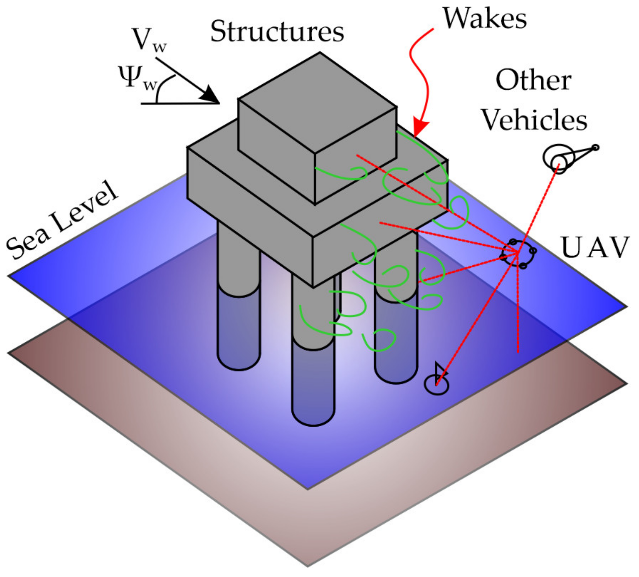
2.1. The Mission
- Initial mission position and goal;
- Geometry of the environment;
- UAS performance capability, e.g., turn rate, climb rate, bank angle, etc.;
- Actuator/sensor performance/degradation;
- Other environmental conditions, e.g., ambient light, sea state, etc. [17]
2.2. Simulation Environment
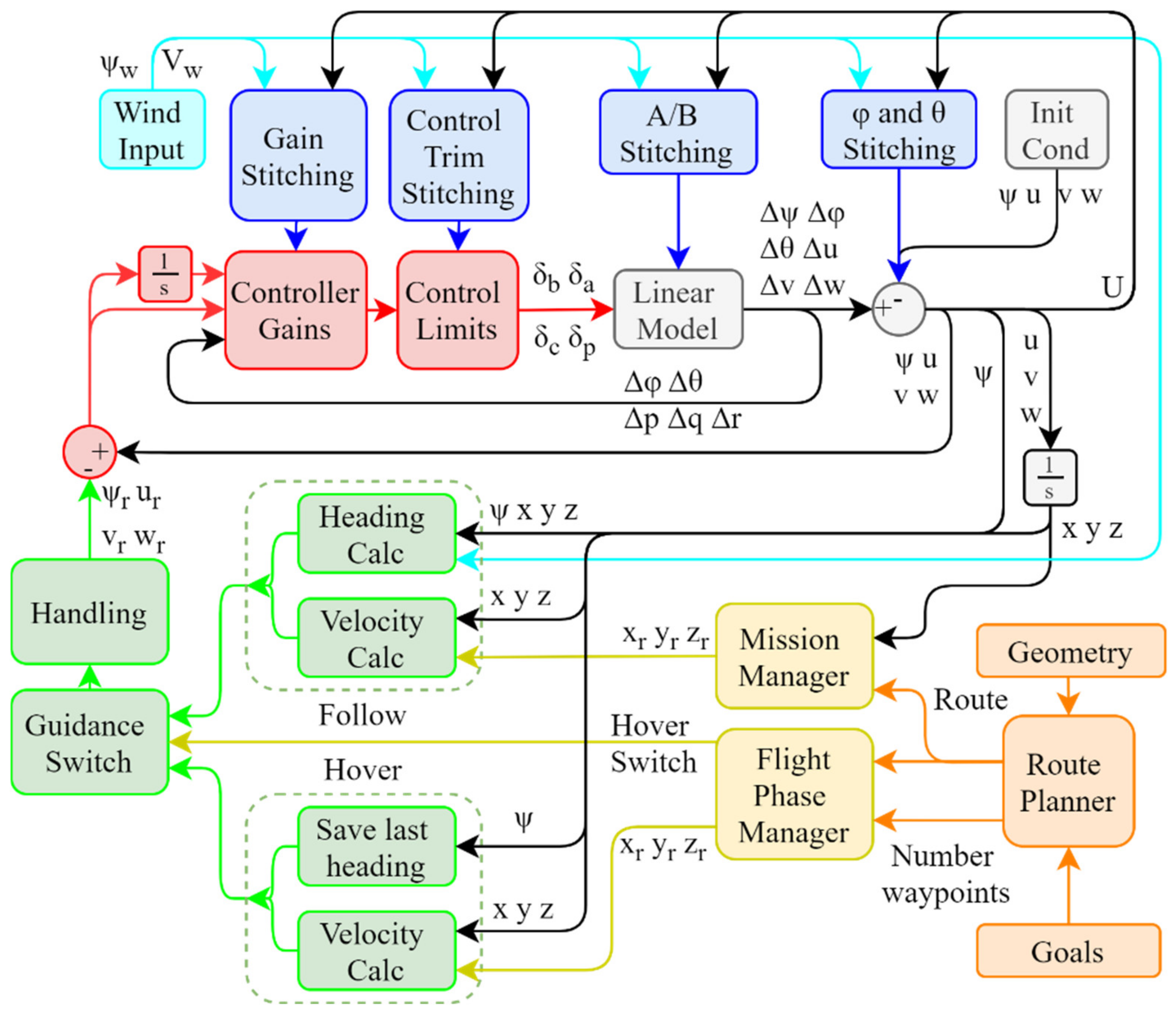
2.2.1. Simulation Architecture
- Stitched Linear Vehicle Model (blue): the air vehicle flight model used for the work described in this paper is a linear model derived from a more complex nonlinear one. To account for changes in vehicle dynamics throughout the flight envelope, these individual linear models are “stitched” together. This process is described in more detail later in the paper.
- Stabilization and Tracking Controller (red): this controller stabilizes the aircraft (a necessary function for the conventional helicopter configuration used) and provides a means for the vehicle model to follow the velocity and heading commands provided by the guidance system.
- Guidance System (green): this system calculates the required velocities and headings to follow the ground track received from the navigation system.
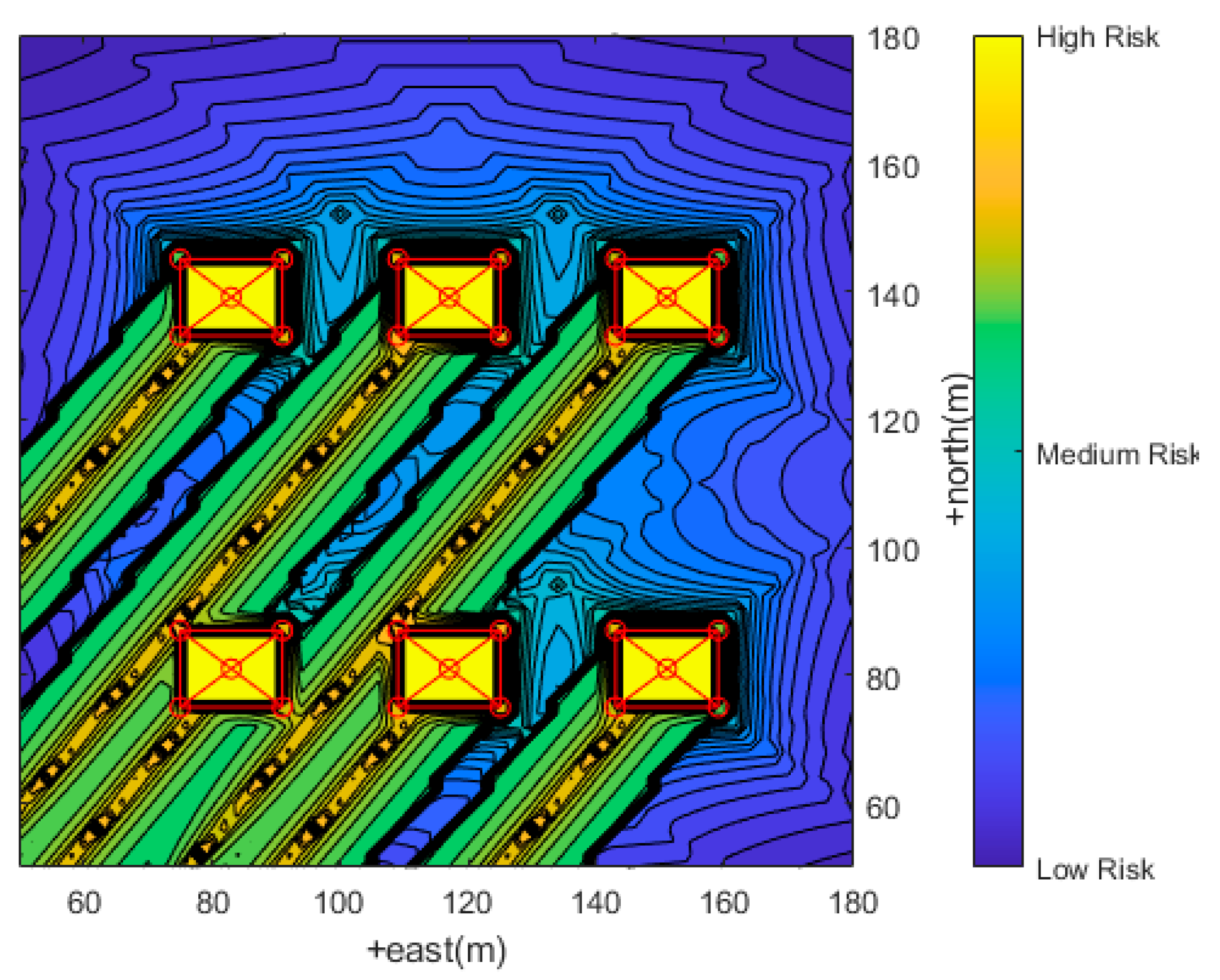
- Navigation System (orange): the navigation system creates a route for the aircraft to follow to achieve the mission, taking into account areas of risk (e.g., turbulent flow in the lee of the structure) and closest point of approach to the asset.
- Mission Management (yellow): in the form reported in this paper, this system is a fairly simple algorithm that decides when to switch to the next waypoint on the route and, once the final mission position has been achieved, when to bring the vehicle to a halt in a hover.
- Dynamics (white): this part of the simulation updates the state of the aircraft from the previous time step based upon the current control inputs.
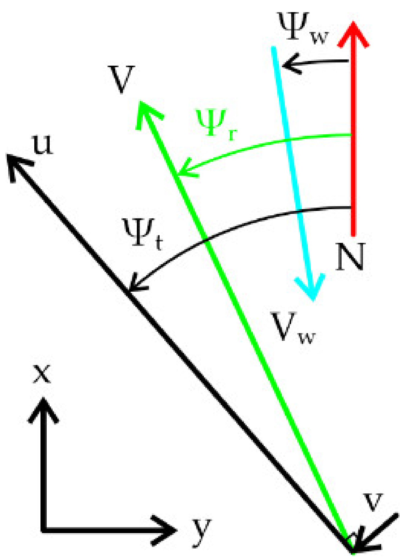
- Wind Model (cyan): this element of the simulation updates the steady wind speed and direction to be used.
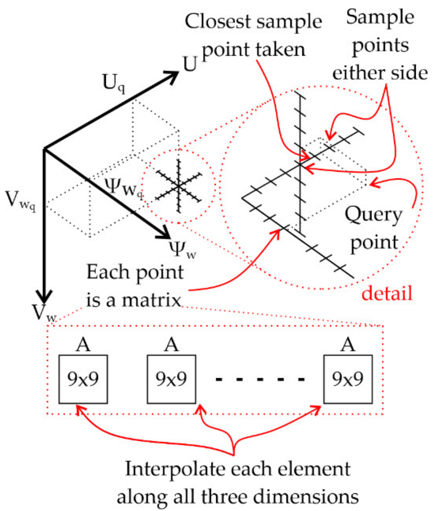
2.2.2. Vehicle Dynamics Linear Model
2.2.3. Vehicle Dynamics Stitching
2.2.4. Stabilization and Tracking Controller Tuning
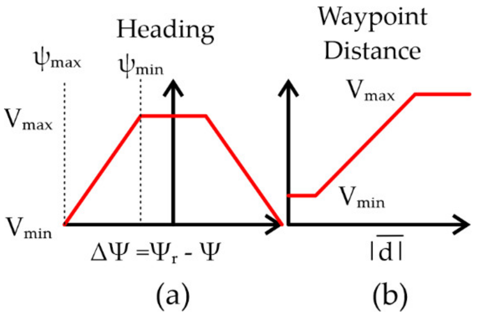
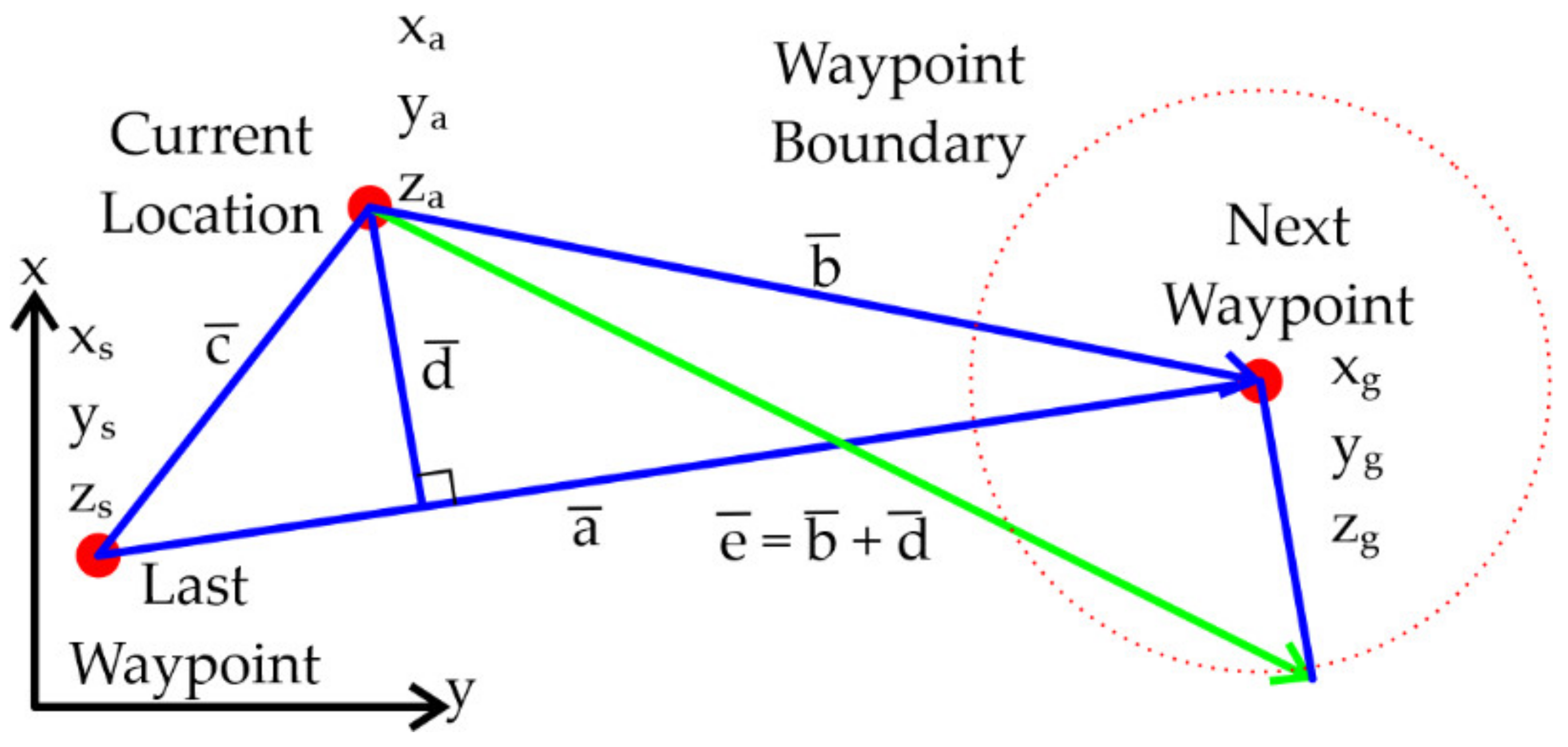
2.2.5. Guidance Command Algorithm
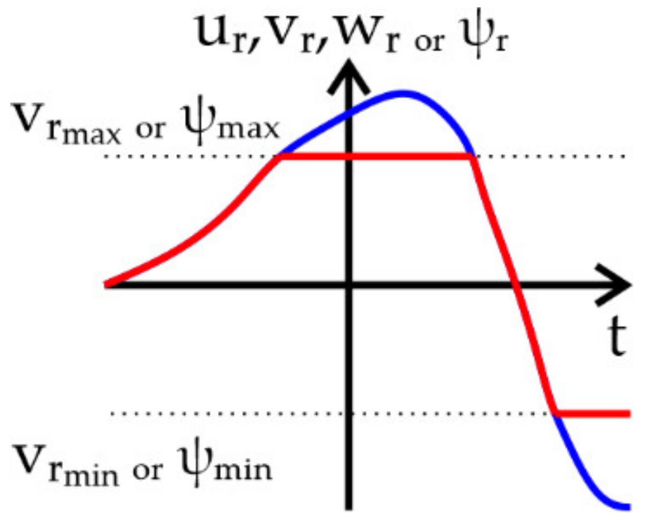
2.2.6. Vehicle Performance Limits
2.2.7. Route Planning
2.2.8. Mission Management
2.3. Performance Metrics
2.3.1. Causes of Mission Failure
2.3.2. Objective Functions for Each Component
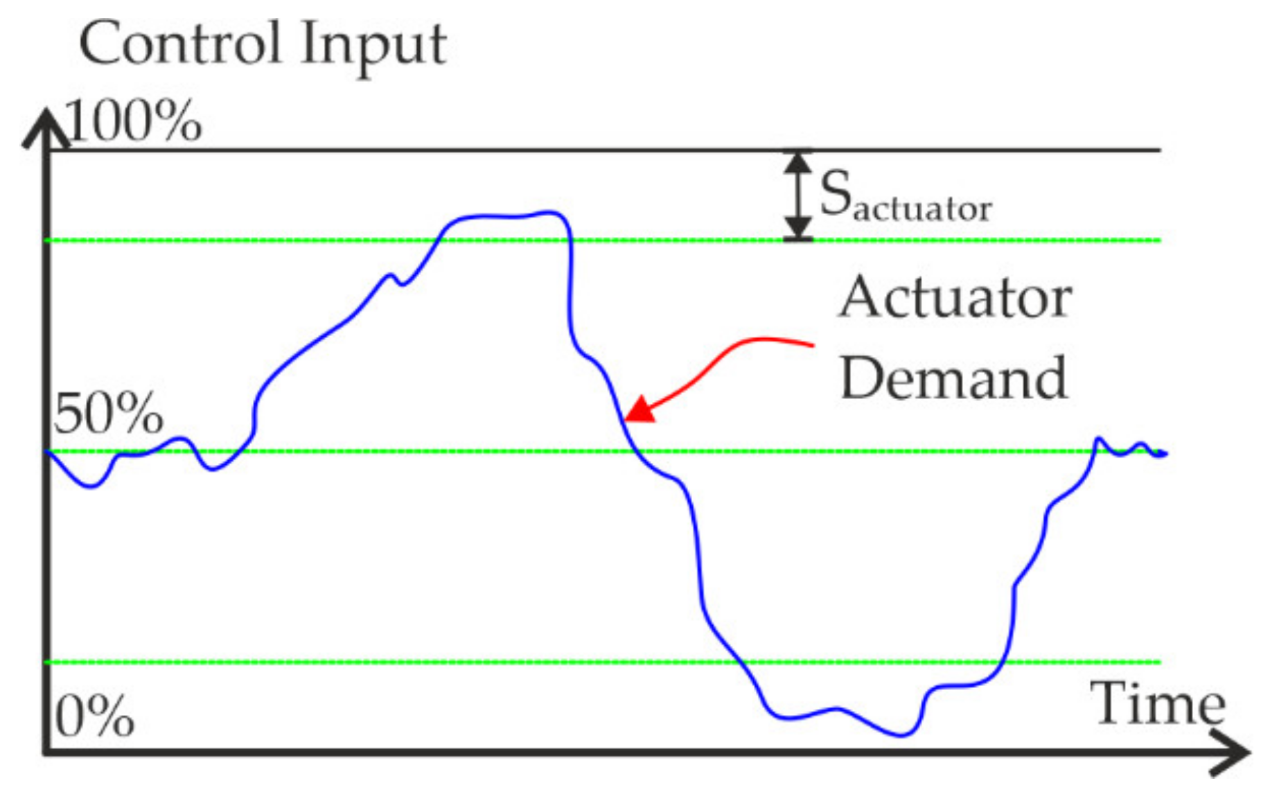
- Actuator: to create the required control response output while leaving a margin of error as a contingency to allow reactions to unforeseen disturbances.
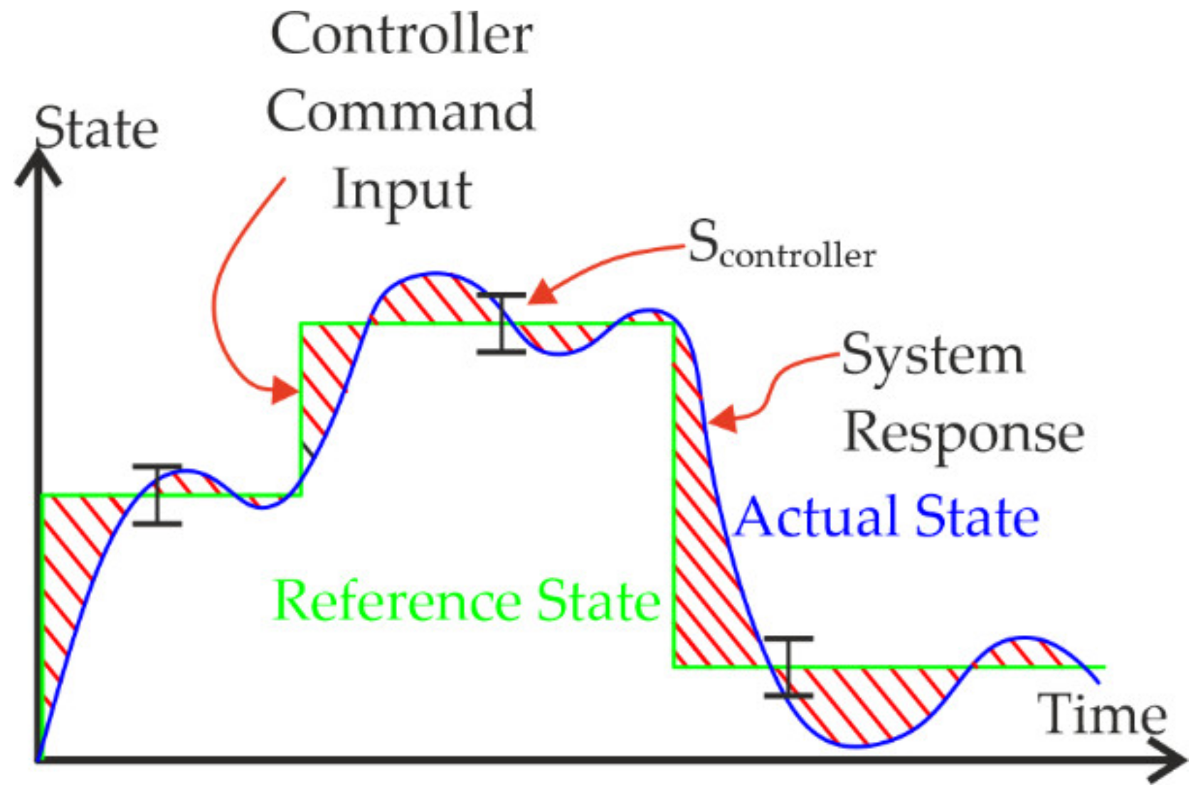
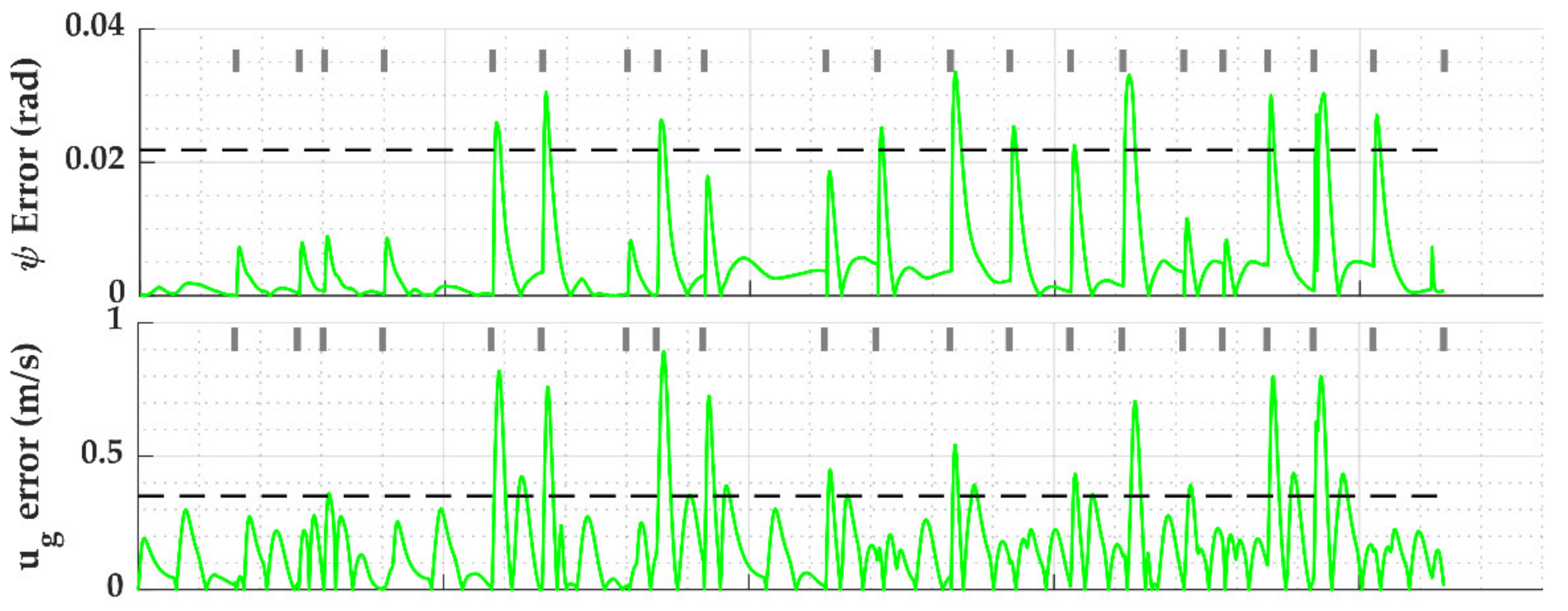
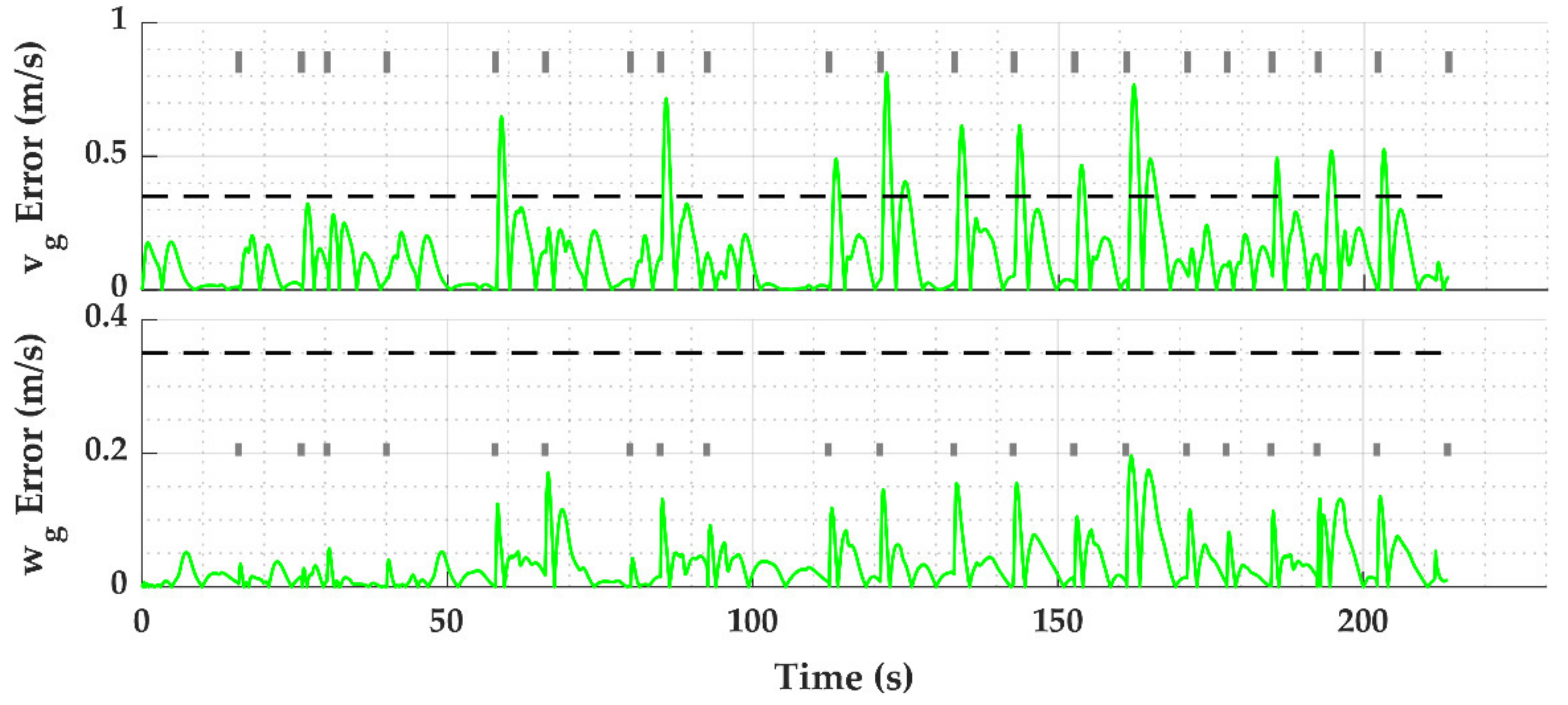
- Controller: to ensure that the current vehicle states follow the commanded states within a user-defined tolerance, defined as the difference between the actual and reference values, while maintaining controlled flight.
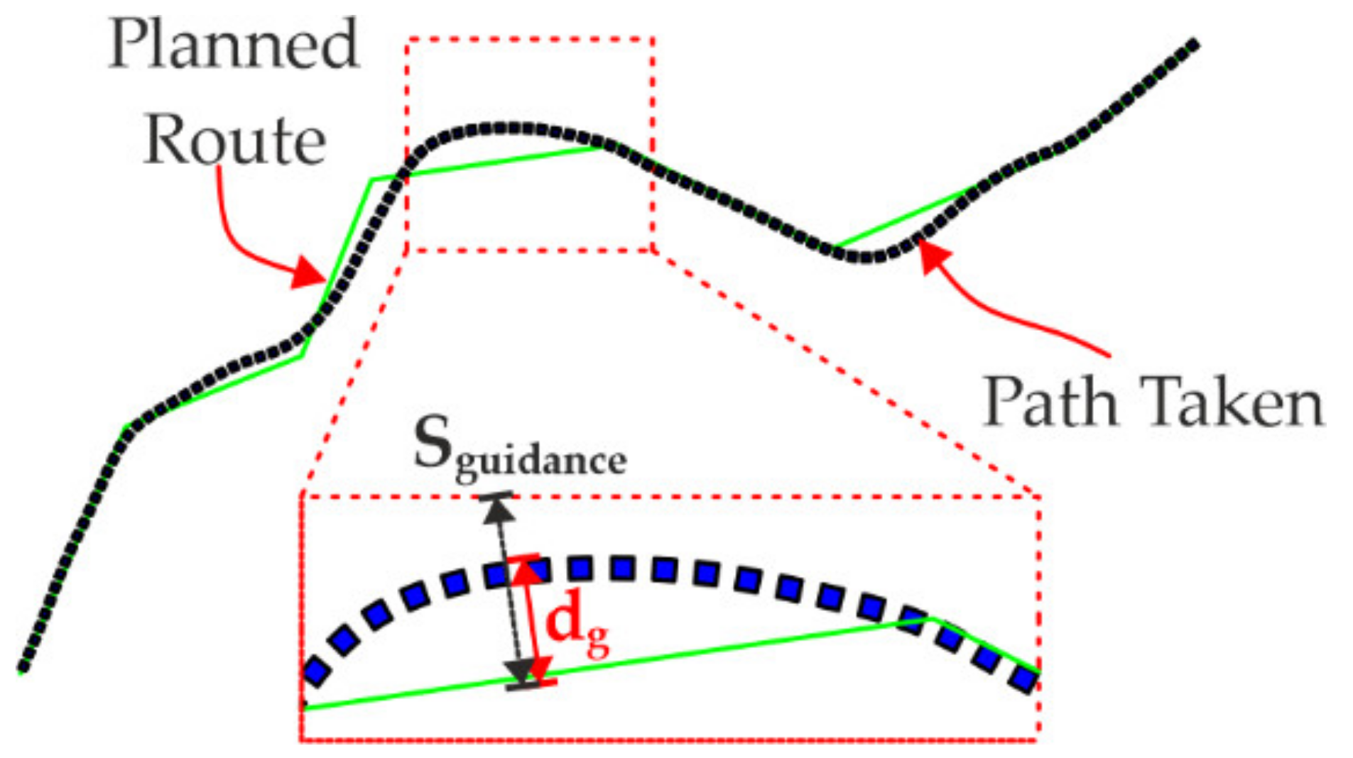
- Guidance: to cause the system to follow the desired path to within a desired separation distance.
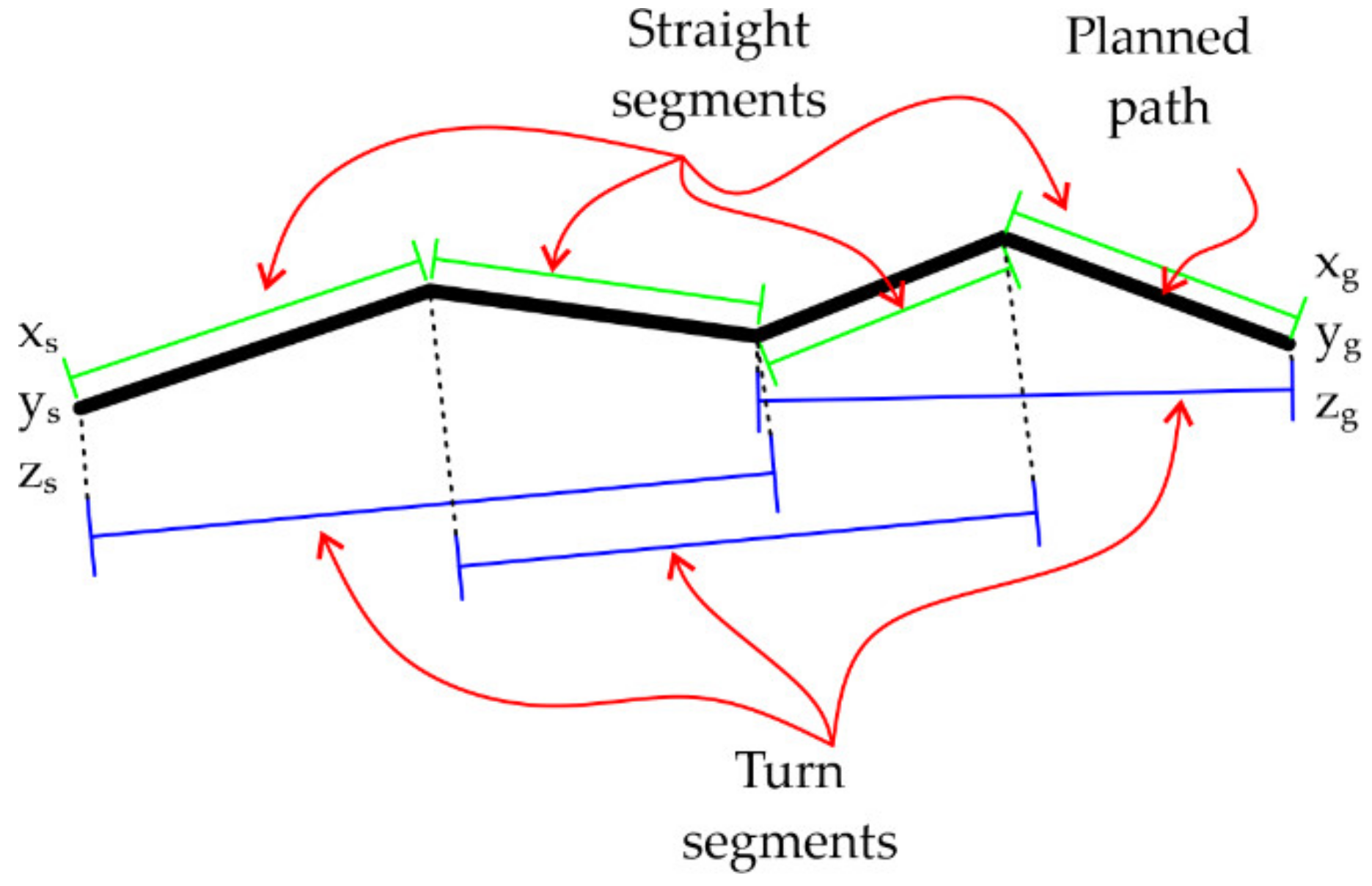
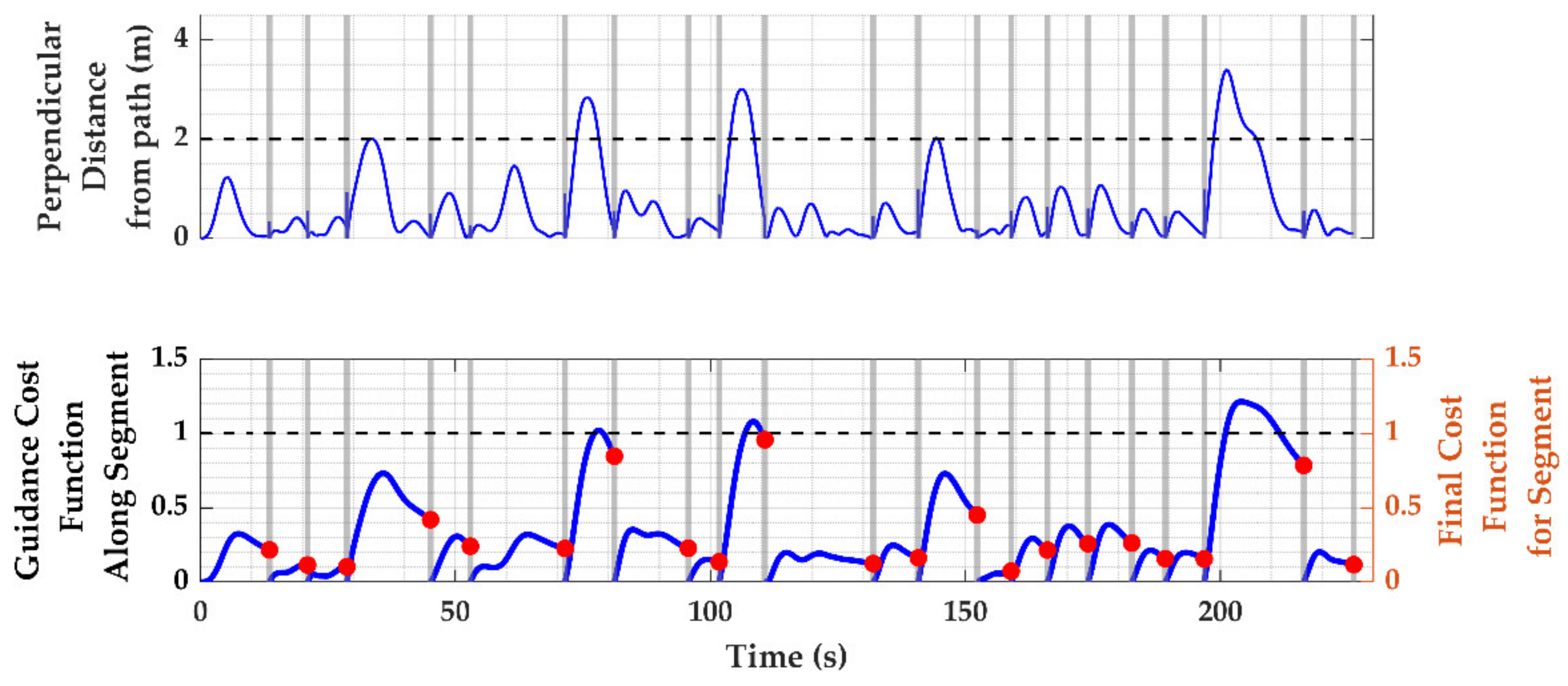
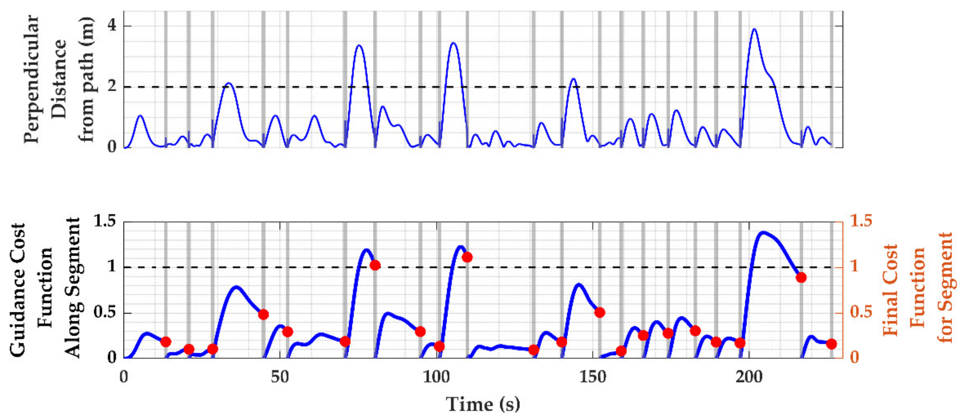
2.3.3. Segmenting the Mission
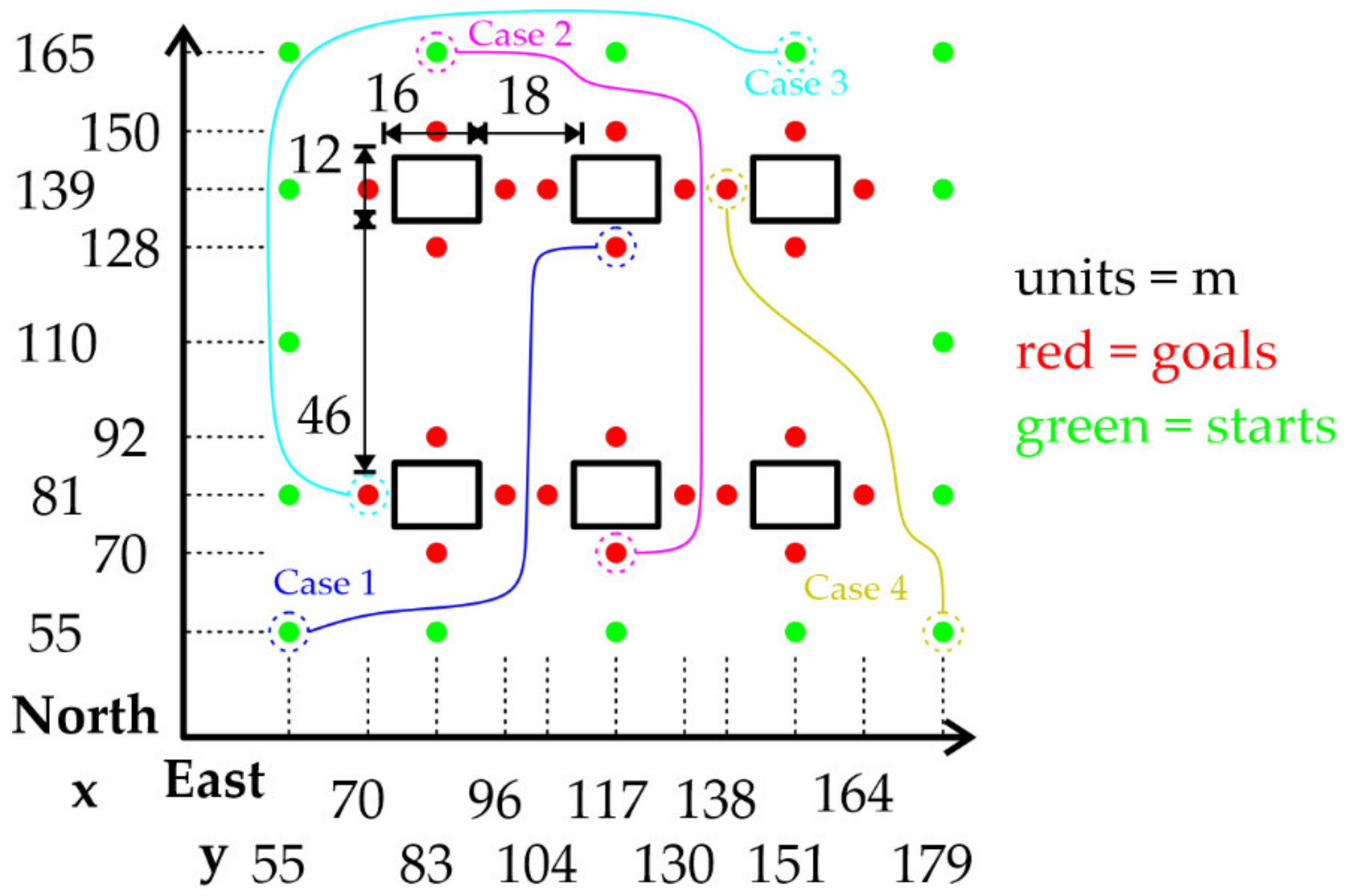
2.4. Experimental Test Matrix
3. Results
3.1. Simulation Performance
3.2. Route Planning Results
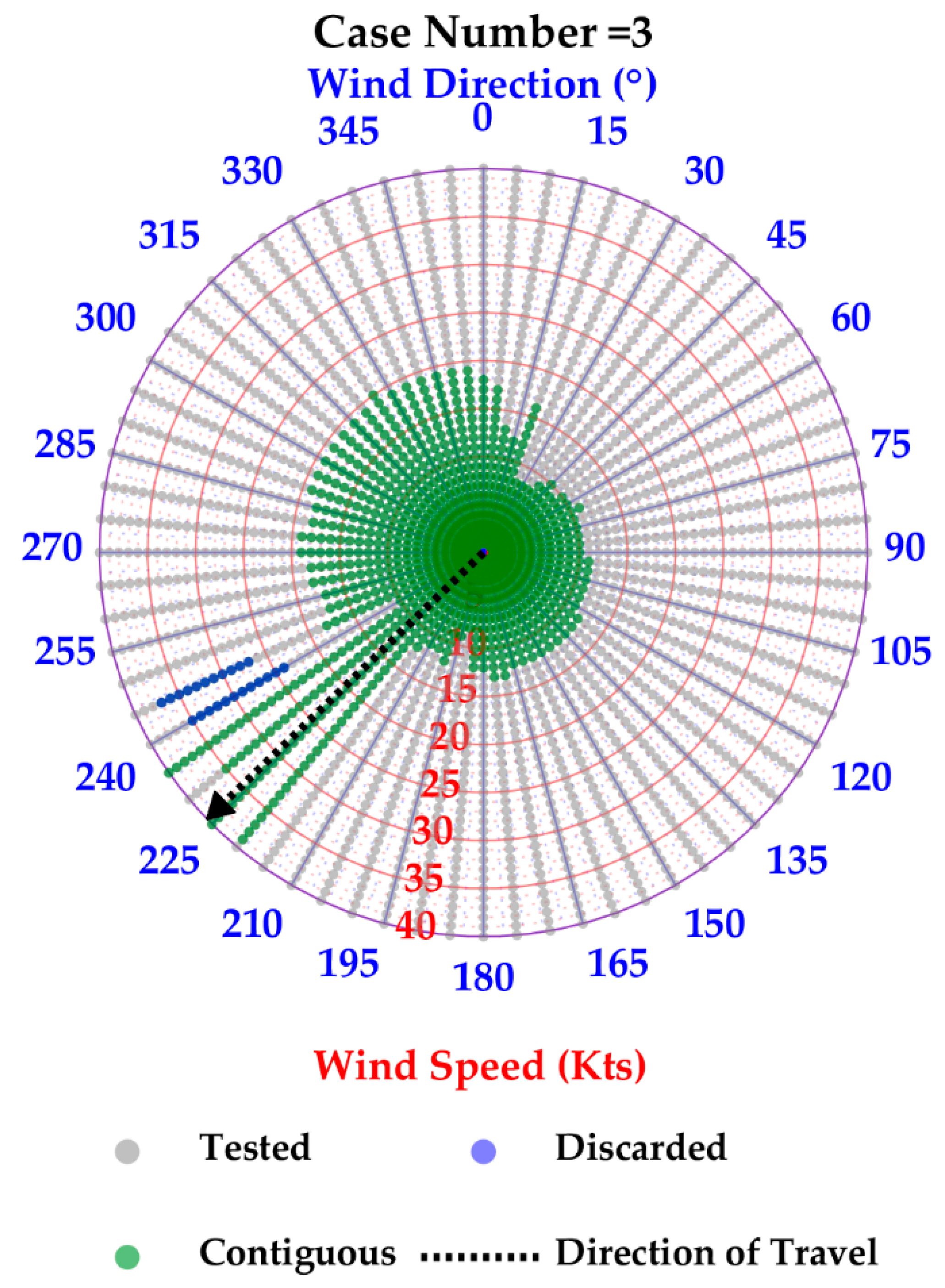
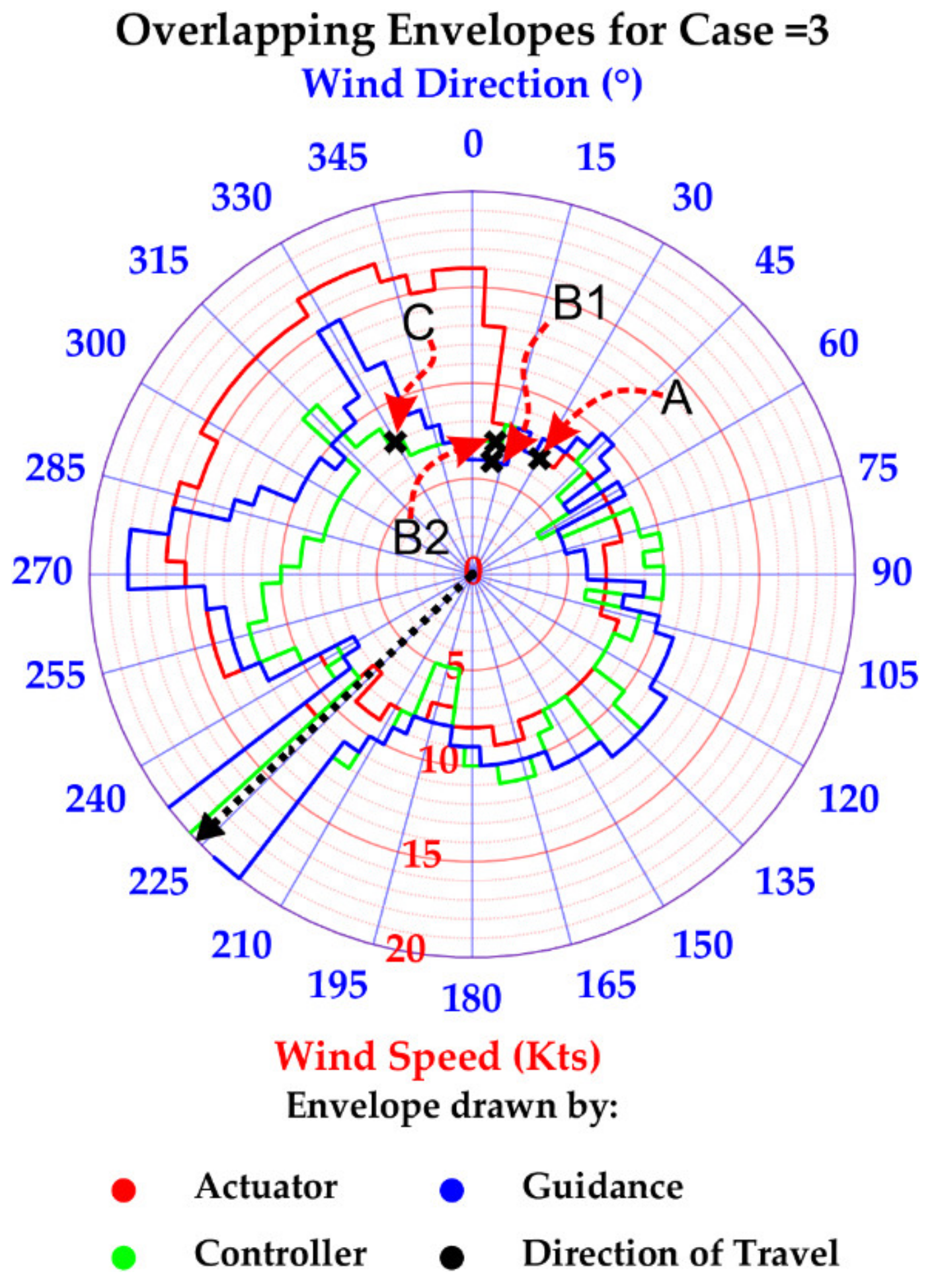
3.3. Simulated Mission Success or Failure
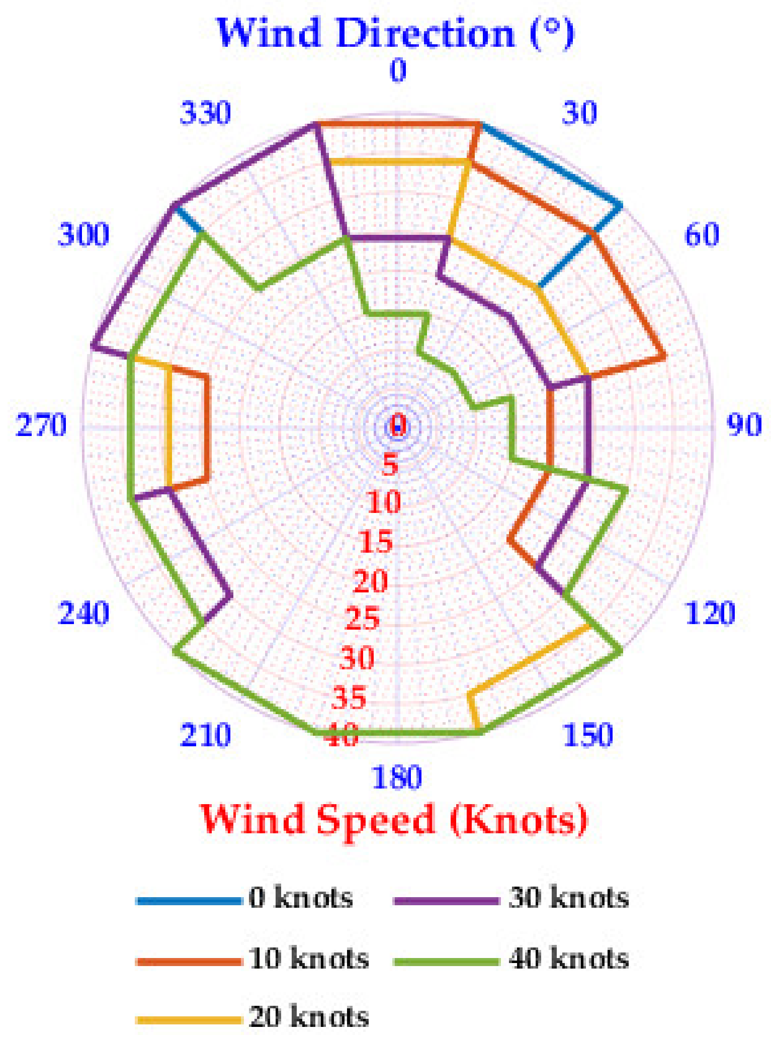
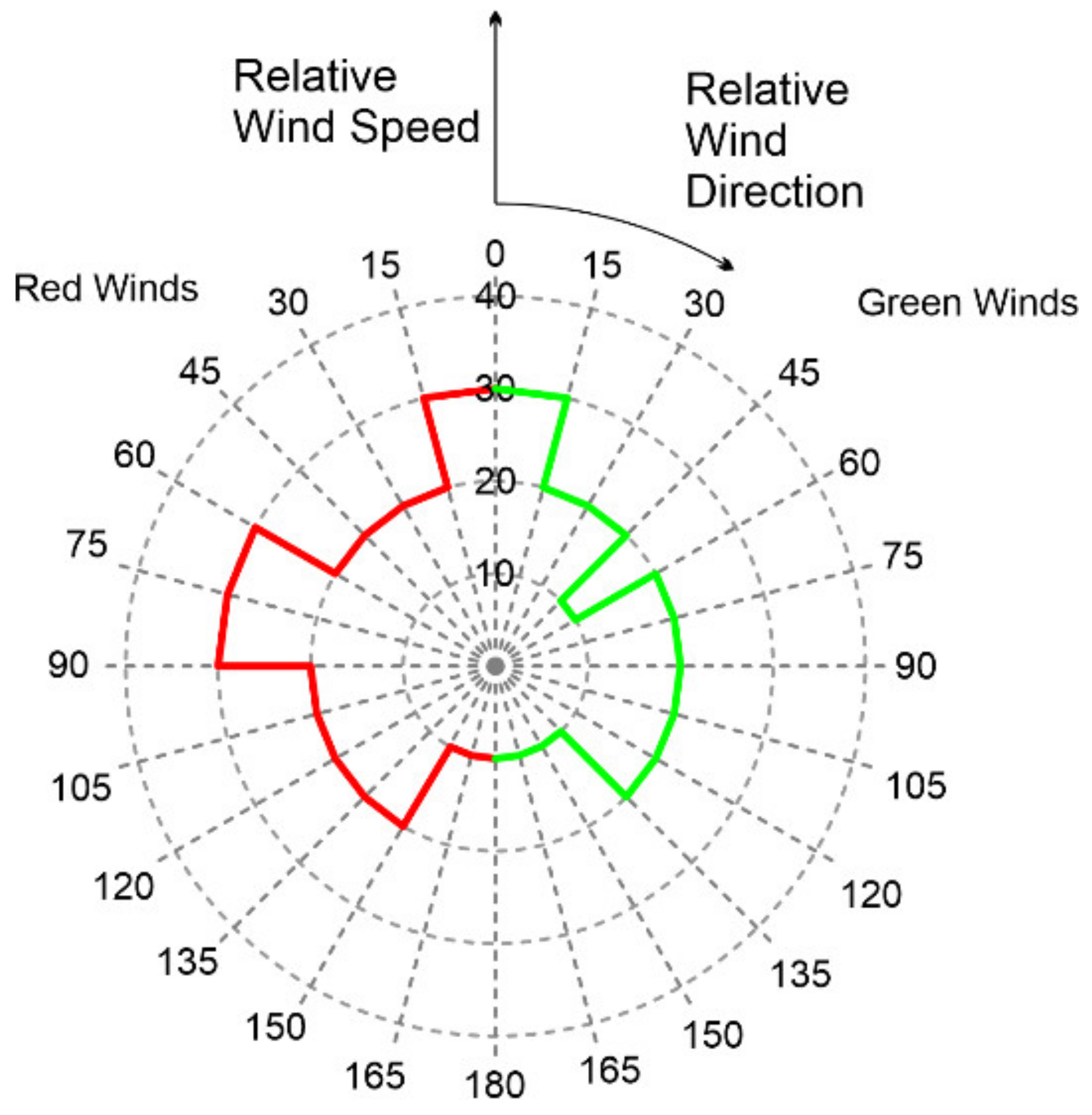
- The green dots represent the contiguous sets of wind conditions for which the mission was completed successfully, i.e., all performance specifications were met.
- The gray dots represent the test points where the mission “failed”; a failed simulation means that the UAS encountered a situation, or was attempting a maneuver, that resulted in a response of the system that exceeded one or more specifications.
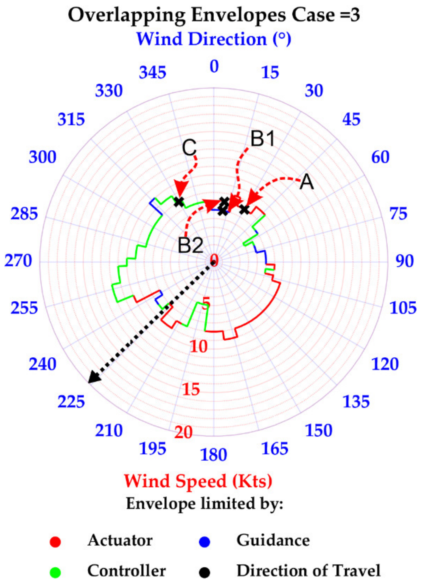
- The blue dots are interesting in that they represent test points that resulted in mission “success”, but that were discarded because there was a gap between those points and the contiguous set of successful mission simulations. It has been assumed that the envelope for a given wind direction must have an unbroken, contiguous set of wind speeds from the zero wind speed condition to the edge of the envelope. This naturally removes the possibility of exclaves of successful simulations or enclaves of failed simulations within the envelope. It also removes possible gaps in the envelope if viewed along a line of increasing wind speed; for example, at a wind direction of 240° in Figure 17. It would not be a safe operation if it had to rely on the wind speed not dropping below a particular value for the mission to succeed.
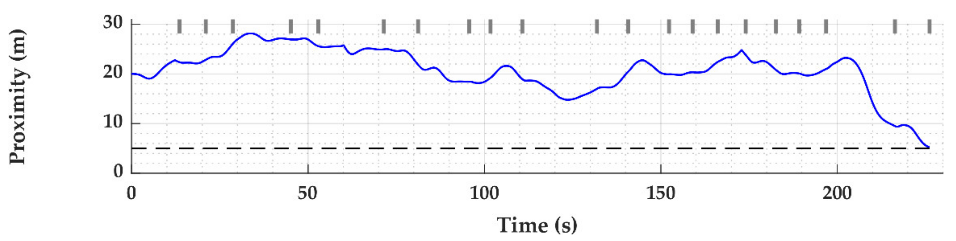
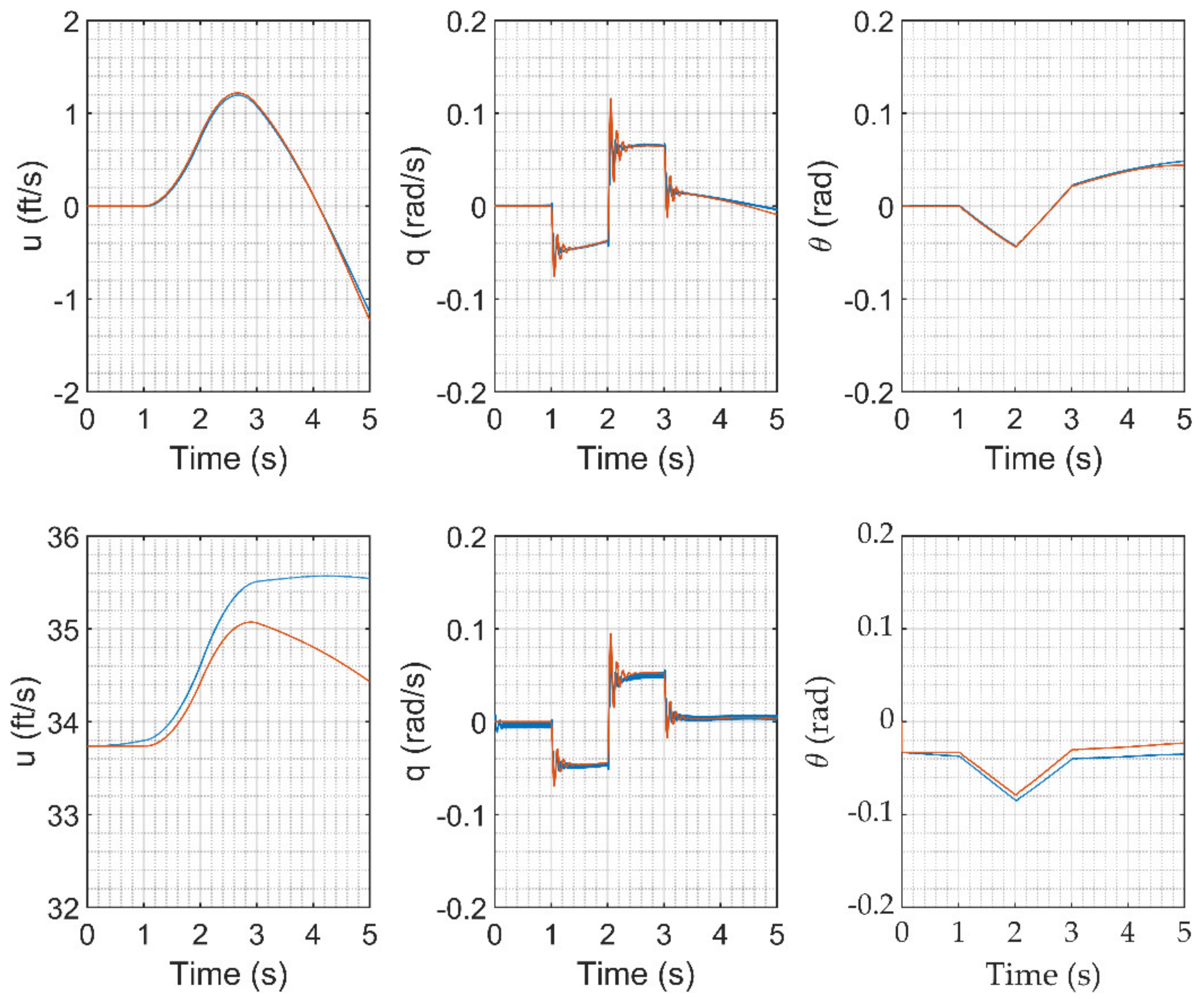
3.4. Test Point Time History Data
3.5. Operating Envelope Creation
3.6. Performance Specification Sensitivity Study
4. Discussion
4.1. Helicopter Operating Limit Envelope for an Offshore Asset Inspection Mission
4.2. Limitations
4.3. General Application
5. Conclusions and Future Work
5.1. Concluding Remarks
- Using both real and simulated manned helicopter–ship operations as an inspiration, operating limit envelopes for the specified vehicle/offshore asset combination can be generated.
- The operating limit envelopes produced provide a condensed, intelligible information regarding the capability of the UAS in the presence of the offshore asset and its corresponding wake. They provide useful information for both system designers and inspection service operators (and onboard flight management systems) alike.
- The use of operating limit techniques for the offshore inspection mission are more complex than the manned helicopter-to-ship case due to the larger number of mission profiles that could potentially be flown.
5.2. Future Work
5.2.1. Nonlinear Dynamics of UAS
5.2.2. Unsteady Wind
5.2.3. Search Algorithm to Find Operating Limit
5.2.4. Optimization of Autonomous System Parameters
5.2.5. Simulation Validation through Real-World Testing
Author Contributions
Funding
Institutional Review Board Statement
Informed Consent Statement
Data Availability Statement
Acknowledgments
Conflicts of Interest
Appendix A


| Symbol | Definition | Units | Symbol | Definition | Units |
|---|---|---|---|---|---|
| Simulation | |||||
| Position components in world frame cartesian axes | Aircraft angular body rates | ||||
| Aircraft actual position components | Aircraft groundspeed in horizontal plane | ||||
| Aircraft body axes | Aircraft true airspeed | ||||
| Aircraft start position components | Wind speed and wind direction | ||||
| Aircraft goal position components | Wind speed components in the inertial frame | ||||
| Aircraft body indicated velocity components in and directions, respectively | Aircraft lateral, longitudinal, collective, and pedal control inputs, respectively | ||||
| Aircraft body ground velocity components in and directions, respectively | Vectors of aircraft groundspeed, wind speed, and wind direction that models were produced at | ||||
| Aircraft orientation in heading, pitch and roll Euler angles, respectively | Query points for groundspeed, wind speed, and wind directions | ||||
| Controller | |||||
| Linear model state and control matrices | LQR method weighting matrices | ||||
| Augmented state and control matrices | A weighting with reference to a particular variable as a subscript | ||||
| A filler matrix used to produce the augmented output matrix | Database of LQR tuned control gains | ||||
| An identity matrix | |||||
| Guidance | |||||
| Generic function identifiers | Unit vector between aircraft start and goal states | ||||
| Partial derivatives of equations and with respect to and | Cross tracking error | ||||
| Step or iteration count | Reference values for aircraft body velocities and heading | ||||
| Vectors between the various aircraft position states | |||||
| Navigation | |||||
| Cost function weightings | Risk metric | ||||
| The Euclidean distance between grid points, and the straight line distance between a grid point and goal | r | Aggregate risk between two points | |||
| Performance Metrics | |||||
| An objective function | Error specification for a subsystem cost function | ||||
| A penalty function | Maximum simulation time | ||||
| A set of parameters | A system state | ||||
| Distance from nearest successful point and perpendicular distance from line between nearest success points | Number of subsystems, actuators, and controller loops, respectively | ||||
| Perpendicular distance from the path | Actual proximity to an obstacle | ||||
| A Pareto function | |||||
| Objective functions for the actuator, controller, guidance and navigation, respectively | |||||
Appendix B


Appendix C

Appendix D
Appendix E


Appendix F
References
- Soubry, A.; Leadsom, A. Oil and Gas Workforce Plan. HM Government. July 2016. Available online: https://assets.publishing.service.gov.uk/government/uploads/system/uploads/attachment_data/file/535039/bis-16-266-oil-and-gas-workforce-plan.pdf (accessed on 7 January 2021).
- Cable, V.; Davey, E.; Moore, M.; Ballard, G. UK Oil and Gas: Business and Goverment Actio. HM Government. March. 2013. Available online: https://assets.publishing.service.gov.uk/government/uploads/system/uploads/attachment_data/file/175480/bis-13-748-uk-oil-and-gas-industrial-strategy.pdf (accessed on 7 January 2021).
- Wooldridge, M. An Introduction to Multiagent Systems, 2nd ed.; John Wiley & Sons: Hoboken, NJ, USA, 2009. [Google Scholar]
- CAP 722 Unmanned Aircraft System Operations in UK Airspace: Guidance; UK Civil Aviation Authority: Gatwick, UK, 2015.
- Huang, H. Autonomy Levels for Unmanned Systems (ALFUS) Framework; National Institute of Standards and Technology: Gaithersburg, MD, USA, 2007.
- Scanlan, J.; Flynn, D.; Lane, D.; Richardson, R.; Richardson, T.; Sobester, A. Extreme Environments Robotics: Robotics for Emergency Response, Disaster Relief and Resilience; UK-RAS Network: Loughborough, UK, 2018. [Google Scholar]
- Carico, G.D.; Fang, R.; Finch, R.S.; Geyer, W.P., Jr.; Krijins, H.W.; Long, K. Helicopter/Ship Qualification Testing: Part 1 Ductch/British Clearance Process. NATO RTO 2003, 22, 13–23. [Google Scholar]
- Forrest, J.S.; Owen, I.; Padfield, G.D.; Hodge, S.J. Ship-Helicopter Operating Limits Prediction Using Piloted Flight Simulation and Time-Accurate Airwakes. J. Aircr. 2012, 49, 1020–1031. [Google Scholar] [CrossRef]
- Finlay, B.A. Ship Helicopter Operating Limit Testing–Past, Present and Future. In Proceedings of the RAeS Rotorcraft Group Conference on ‘Helicopter Operations in the Maritime Environment’, London, UK, 7–8 November 2001. [Google Scholar]
- Advani, S.K.; Wilkinson, C.H. Dynamic Interface Modelling and Simulation: A Unique Challenge. In Proceedings of the Royal Aeronautical Society Conference on Helicopter Flight Simulation, Royal Aeronautical Soc. (RAeS), London, UK, 7–8 November 2001. [Google Scholar]
- Healey, J.V. Simulating the Helicopter-Ship Interface as an Alternative to Current Methods of Determining the Safe Operating Envelopes; Naval Postgraduate School: Monterey, CA, USA, 1986; pp. 48–58. [Google Scholar]
- Roscoe, M.F.; Wilkinson, C.H. DIMSS-JSHIP’s M&S Process for Ship Helicopter Testing and Training. In Proceedings of the AIAA Modeling and Simulation Technologies Conference and Exhibit, Monterey, CA, USA, 5–8 June 2002. [Google Scholar]
- Owen, I.; White, M.; Padfield, G.D.; Hodge, S.J. A virtual engineering approach to the ship-helicopter dynamic interface–A decade of modelling and simulation research at the University of Liverpool. Aeronaut. J. 2017, 121, 1833–1857. [Google Scholar] [CrossRef] [Green Version]
- Hodge, S.J.; Forrest, J.; Padfield, G.D.; Owen, I. Simulating the Environment at the Helicopter-Ship Dynamic Interface: Research, Development and Application. Aeronaut. J. 2012, 116, 1155–1184. [Google Scholar] [CrossRef]
- Kelly, M.; Watson, N.A.; Hodge, S.J.; White, M.D.; Owen, I. The Role of Modelling and Simulation in the Preparations for Flight Trials Aboard the Queen Elizabeth Class Aircraft Carriers. In Proceedings of the 14th International Naval Engineering Conference, Glasgow, UK, 2–4 October 2018; Available online: https://doi.org/10.24868/issn.2515-818X.2018.037 (accessed on 7 January 2021).
- Memon, W.A.; Owen, I.; White, M.D. SIMSHOL: A Predictive Simulation Approach to Inform Helicopter–Ship Clearance Trials. AIAA 2020, 57, 854–875. [Google Scholar] [CrossRef]
- Page, P.; Webster, M.; Fisher, M.; Jump, M. Towards a Methodology to Test UAVs in Hazardous Environments. In Proceedings of the ICAS 2019, The Fifteenth International Conference on Autonomic and Autonomous Systems, Athens, Greece, 2–6 June 2019; pp. 38–45. [Google Scholar]
- Fell, T.R.; White, M.D.; Owen, I. Sensitivity study of a small maritime rotary UAS operating in a turbulent airwake. In Proceedings of the 71st AHS Forum, Virginia Beach, VA, USA, 27–29 May 2015. [Google Scholar]
- Val, R.D.; He, C. Validation of the FLIGHTLAB Virutal Engineering Toolset. Aeronaut. J. 2018, 122, 519–555. [Google Scholar] [CrossRef]
- Padfield, G.D. Helicopter Flight Dynamics, 1st ed.; Blackwell Science Ltd.: London, UK, 1996. [Google Scholar]
- Furgeson, D.; Likhachev, M.; Stentz, A. A guide to heuristic-based Path Planning. In Proceedings of the ICAPS’05 15th International Conference on Automated Planning & Scheduling, Monterey, CA, USA, 5–10 June 2005. [Google Scholar]
- Moss CS50 MKII Oil Platform. Available online: https://grabcad.com/library/moss-cs50-mkii-oil-platform (accessed on 7 January 2021).
- Webster, M.; Western, D.; Araiza-Illan, D.; Dixon, C.; Eder, K.; Fisher, M.; Pipe, A. A Corroborative Approach to Verification and Validation of Human-Robot Teams. Int. J. Robot. Res. 2020, 39. [Google Scholar] [CrossRef]
- Fisher, M.; Cardoso, R.C.; Collins, E.C.; Dadswell, C.; Dennis, L.A.; Dixon, C.; Farrell, M.; Ferrando, A.; Huang, X.; Jump, M.; et al. An Overview of Verification and Validation Challenges for Inspection Robots. Robotics 2021, 10, 67. [Google Scholar] [CrossRef]
- Shima, T.; Rasmussen, S. UAV Cooperative Decision and Control: Challenges and Practical Approaches; Society for Industrial and Applied Mathematics: Philadelphia, PA, USA, 2009. [Google Scholar]


| Operating Condition | Range of Values (Min:Delta:Max) |
|---|---|
| Forward Velocity U | −20:5:40 |
| Wind Speed Vw | 0:5:40 |
| Wind Direction , | 0:30:330 |
| Variable | Range | Step | Total Variations | Total Combinations |
|---|---|---|---|---|
| Wind Speed (knots) | 40 | 2880 | ||
| Wind Direction (deg) | 72 |
| Case Number | Start | Goal | Num Sims |
|---|---|---|---|
| 1 | [55 55] | [128 117] | 2880 |
| 2 | [165 83] | [70 117] | 2880 |
| 3 | [165 151] | [81 70] | 2880 |
| 4 | [55 179] | [139 138] | 2880 |
| Total | 11,520 |
| Performance Specification | Range | Step | Total Variations |
|---|---|---|---|
| Actuator (%) | 5 | ||
| Controller Heading (°) | 5 | ||
| Controller Velocity (m/s) | 5 | ||
| Guidance (m) | 5 |
| m/s |
| m |
| Processor | AMD Ryzen 9 3950X |
| Cores | 16 |
| Speed | 3.5 GHz |
| Logical Processors | 32 |
| RAM | Corsair 32GB Vengeance LPX DDR4 3200MH |
| Memory | 64 GB |
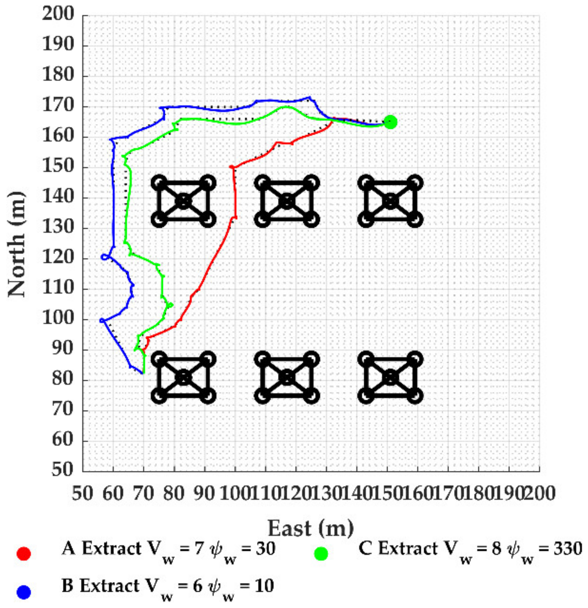
| Test Point | Wind Speed | Wind Direction |
|---|---|---|
| A | 7 | 30 |
| B1 | 6 | 10 |
| B2 | 7 | 10 |
| C | 8 | 330 |
Publisher’s Note: MDPI stays neutral with regard to jurisdictional claims in published maps and institutional affiliations. |
© 2021 by the authors. Licensee MDPI, Basel, Switzerland. This article is an open access article distributed under the terms and conditions of the Creative Commons Attribution (CC BY) license (https://creativecommons.org/licenses/by/4.0/).
Share and Cite
Page, V.; Dadswell, C.; Webster, M.; Jump, M.; Fisher, M. Towards the Determination of Safe Operating Envelopes for Autonomous UAS in Offshore Inspection Missions. Robotics 2021, 10, 97. https://doi.org/10.3390/robotics10030097
Page V, Dadswell C, Webster M, Jump M, Fisher M. Towards the Determination of Safe Operating Envelopes for Autonomous UAS in Offshore Inspection Missions. Robotics. 2021; 10(3):97. https://doi.org/10.3390/robotics10030097
Chicago/Turabian StylePage, Vincent, Christopher Dadswell, Matt Webster, Mike Jump, and Michael Fisher. 2021. "Towards the Determination of Safe Operating Envelopes for Autonomous UAS in Offshore Inspection Missions" Robotics 10, no. 3: 97. https://doi.org/10.3390/robotics10030097
APA StylePage, V., Dadswell, C., Webster, M., Jump, M., & Fisher, M. (2021). Towards the Determination of Safe Operating Envelopes for Autonomous UAS in Offshore Inspection Missions. Robotics, 10(3), 97. https://doi.org/10.3390/robotics10030097