
Maize Internode Autofluorescence at the Macroscopic Scale: Image Representation and Principal Component Analysis of a Series of Large Multispectral Images


Abstract
1. Introduction
2. Materials and Methods
2.1. Samples
2.1.1. Maize Inbred Lines
2.1.2. Internode Cross-Sections
2.2. Image Acquisition
2.2.1. Multispectral Autofluorescence Imaging
2.2.2. Multispectral Images and Pseudospectra
- Multispectral images
- Pseudospectra
2.3. Image Processing
2.3.1. Image Representation
- -
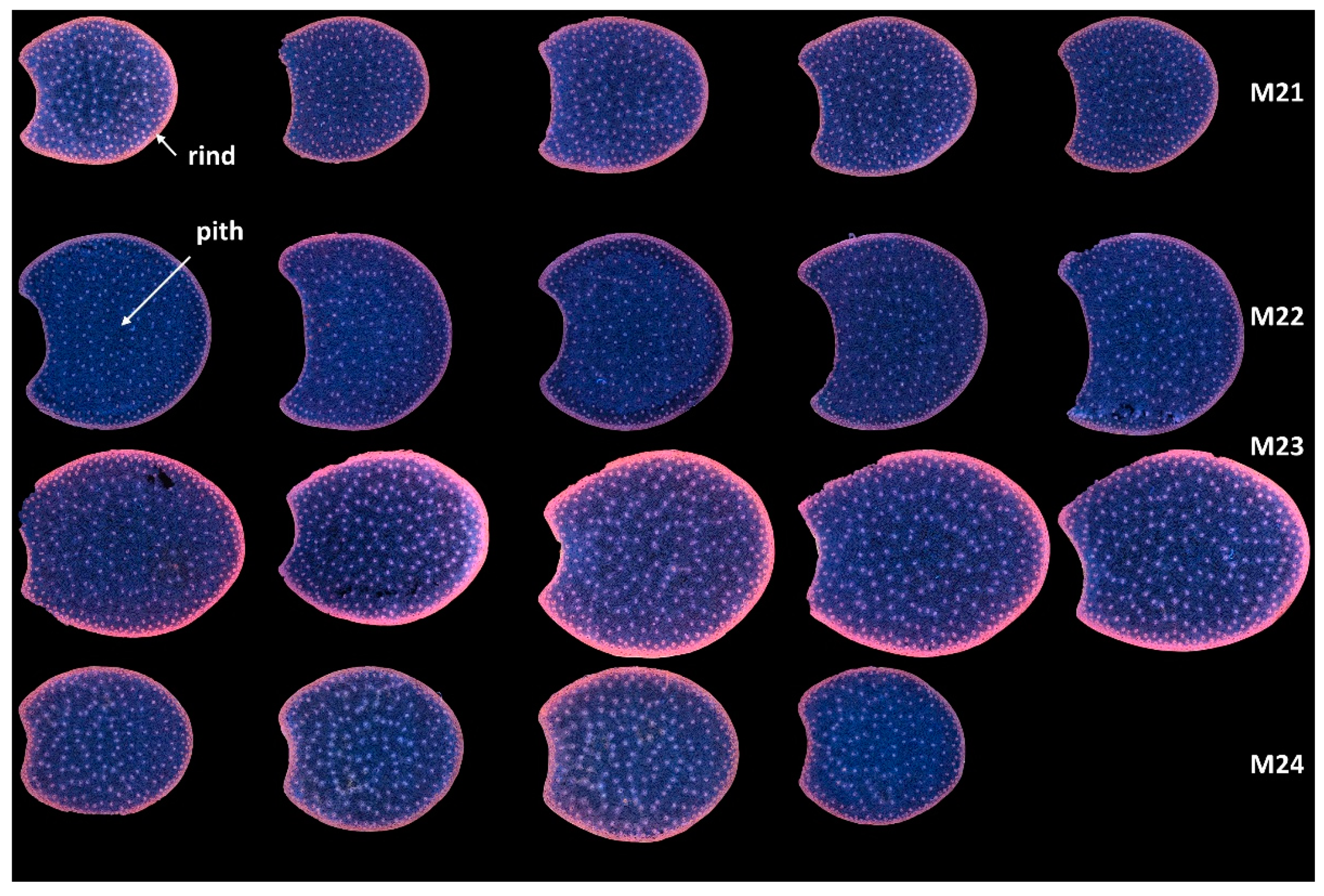
- RGB composite images of macrofluorescence
- -
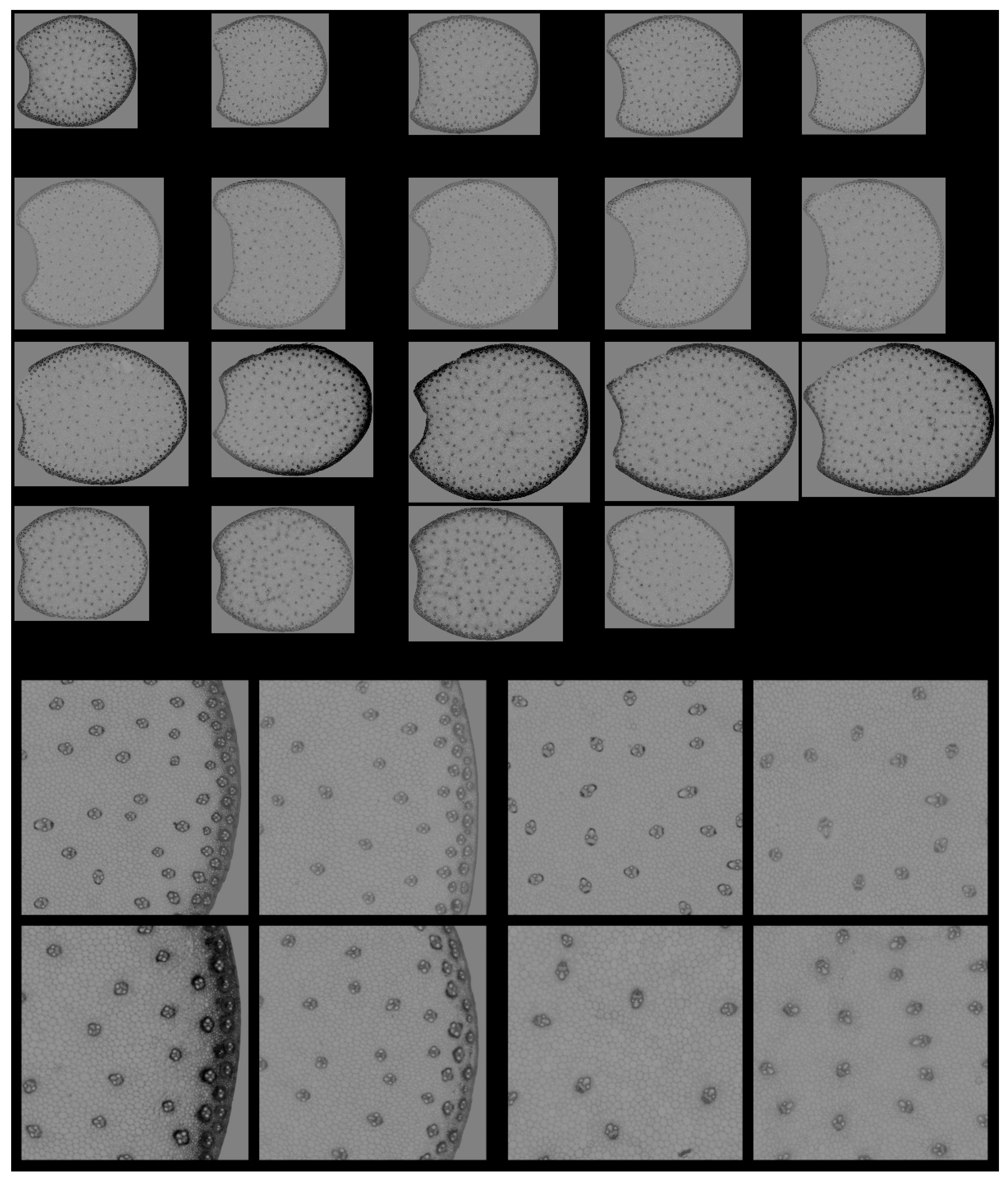
- Determining a common greyscale
- -
- From series to detail: a multiscale representation
2.3.2. Regions of Interest of the Internode Sections
2.3.3. Principal Component Analysis of a Series of Large Multispectral Images
- -
- the local number of pixels ni contained in the data table Xi,
- -
- the local sum of all pseudospectra si:
- -
- the local contribution to the variance/covariance matrix is as follows:
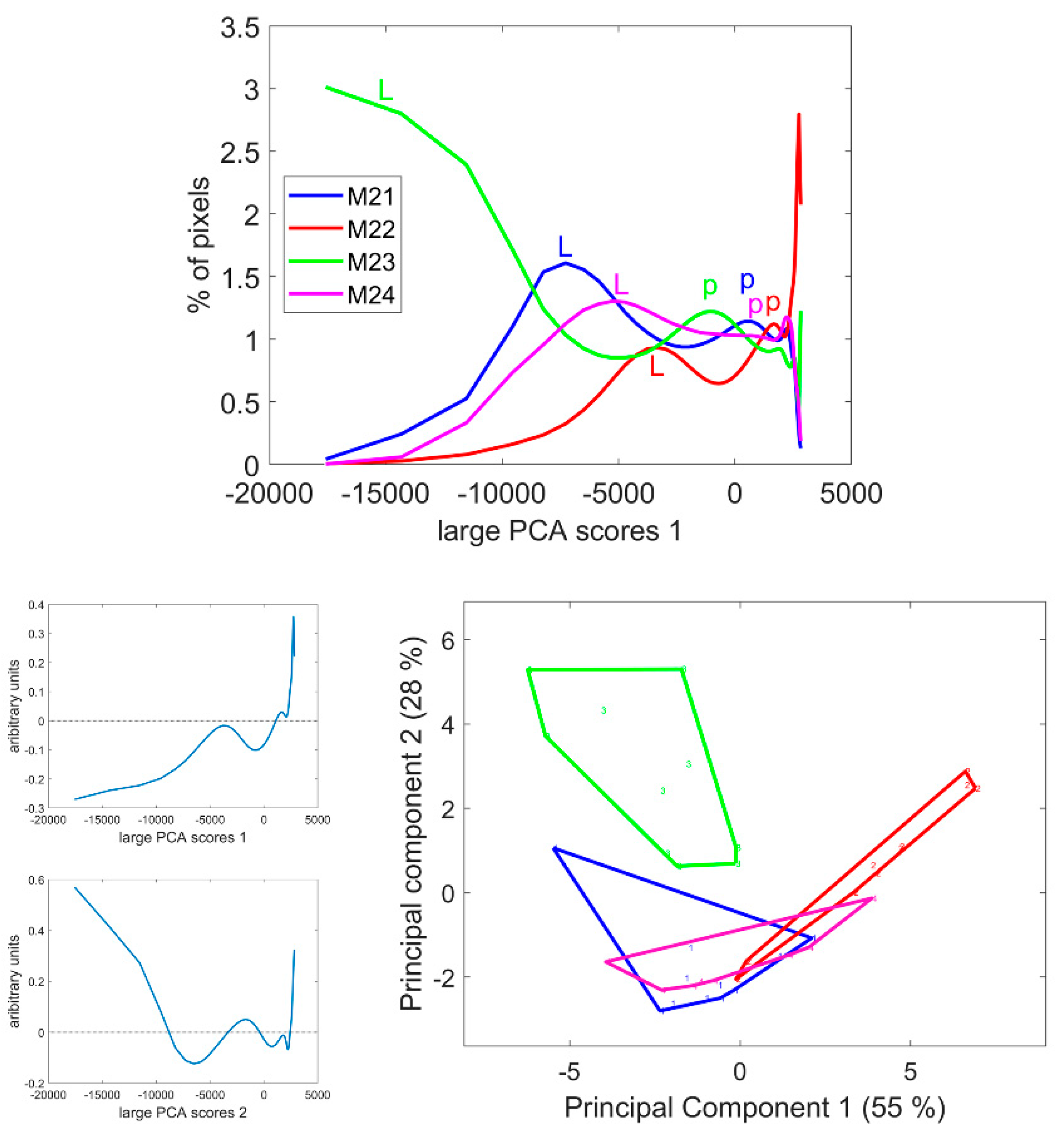
2.3.4. Representation of Large PCA Scores
2.3.5. Distribution of Large PCA Scores
- Step 1, during large PCA score computing:
- -
- A large number of bins is a priori fixed with linear edges between each bin. The minimum and maximum edges are determined by considering the eigenvalue λ(i) of each component. A multiplicative factor is applied to the eigenvalue large enough to a priori include a maximum number of pixels with extreme scores. The minima were a priori set to −25 × λ(i), the maxima to +25 × λ(i) and the number of bins to 10,000.
- -
- For each multispectral image, scores are computed as described in Section 2.3.3, and the score distributions are calculated immediately afterwards. The minimum and maximum edges can be updated if the minimum or maximum scores exceed the a priori values.
- -
- The series of distributions is saved at the end of the image series processing.
- Step 2, postprocessing of the score distributions:
- -
- For each large PCA component, the total score distribution is calculated by summing up all individual image score distributions. The cumulative distribution, called the total cumulative score distribution, is computed.
- -
- The percentiles of the total cumulative score distribution are next calculated. Here, percentiles corresponding to 0 to 100% of the pixels per step of 1% were considered.
- -
- The percentiles defined new edges, leading to bins with variable widths.
- -
- Finally, the new edges were used to interpolate the cumulative score distribution for each image and to calculate the corresponding score distribution.
2.4. Analysis of the Large PCA Score Distributions
3. Results
3.1. Exploring the Variability through Image Series Representation
3.1.1. Montage of Image Series
3.1.2. Example Images
3.2. Average Pseudospectra
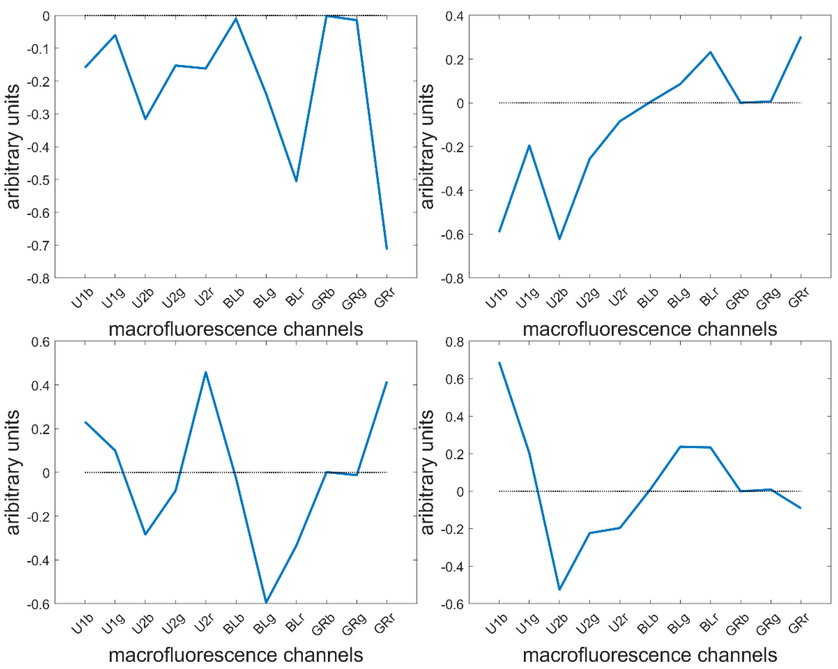
3.3. Large Principal Component Analysis: loadings
3.4. Large Principal Component 1: General Intensity Variations
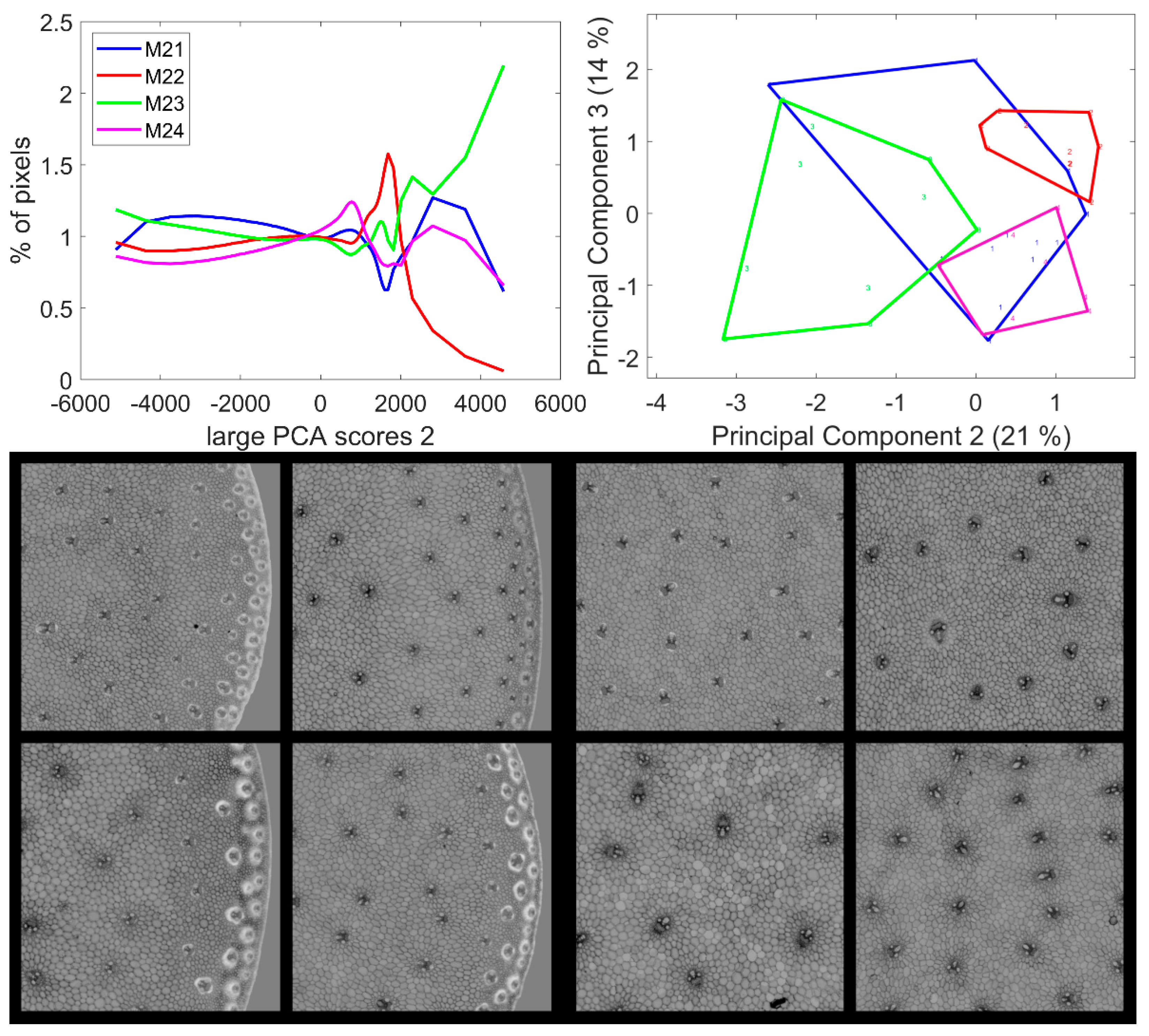
3.5. Large Principal Component 2: UV and Visible Fluorescence
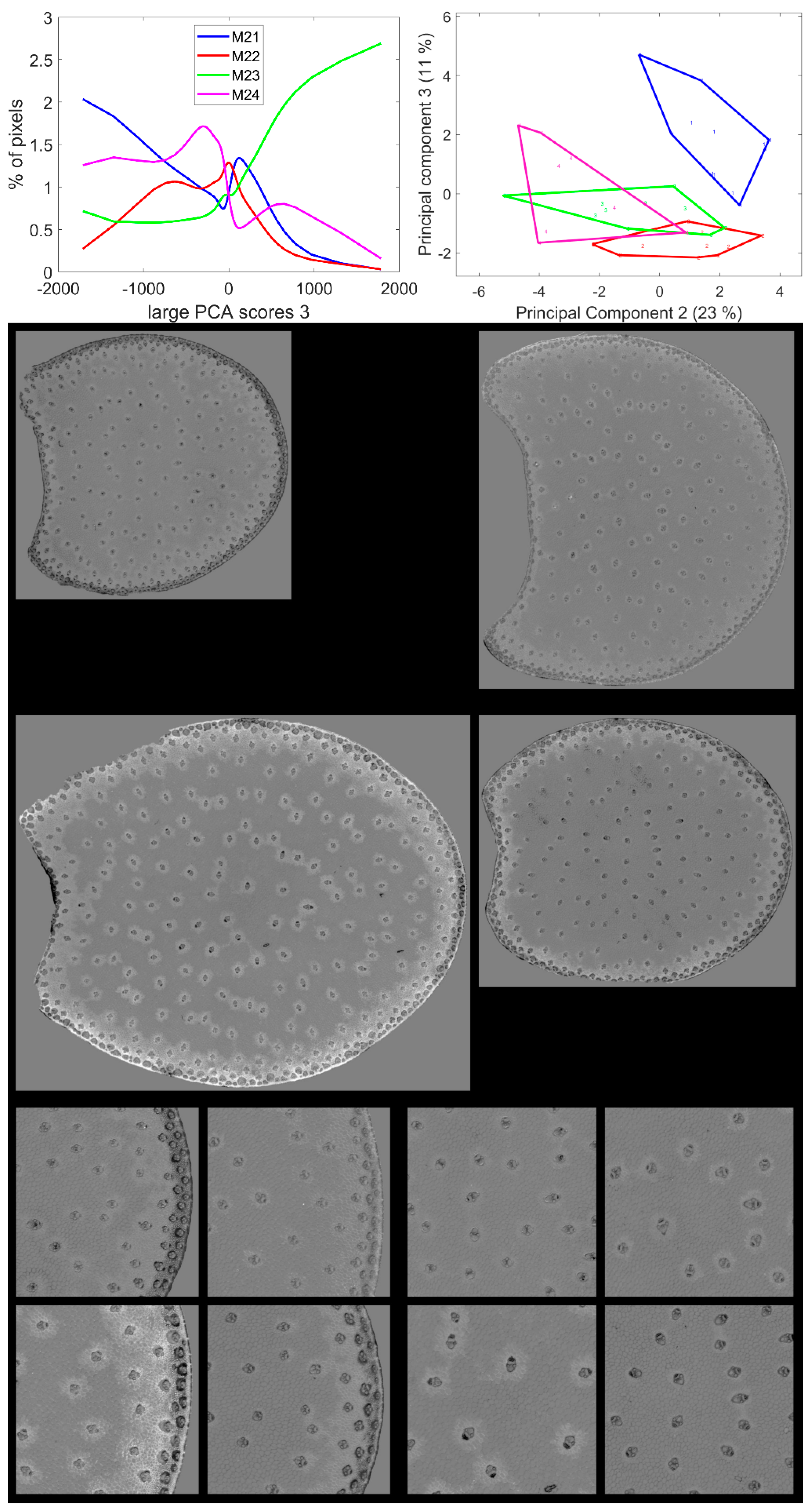
3.6. Large Principal Component 3: BLUE Excitation and UV–GREEN-Induced Red Emission
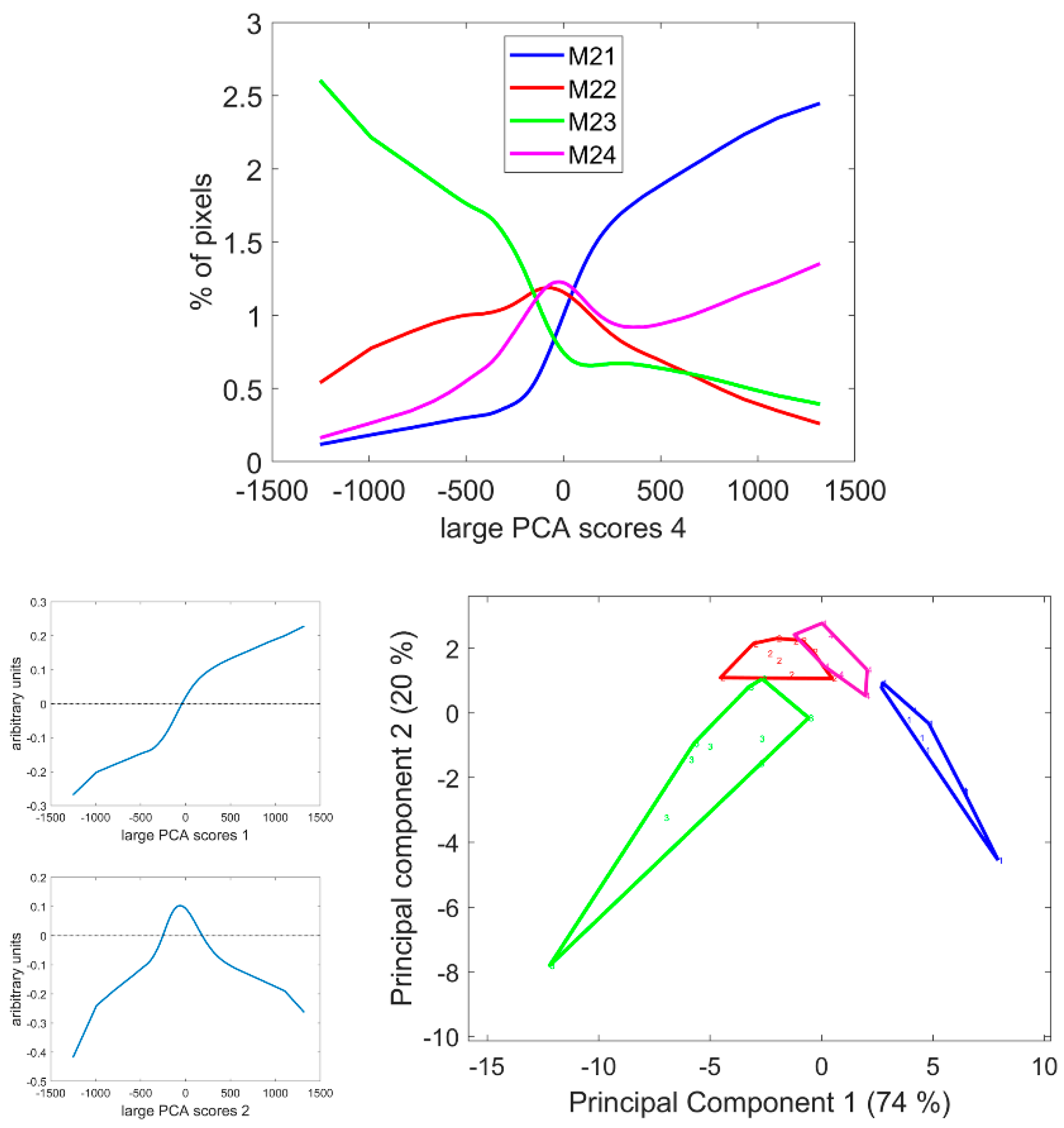
3.7. Large Principal Component 4: UV1 and UV2 Fluorescence Behaviour
4. Discussion
4.1. Multispectral Autofluorescence Imaging to Evaluate the Distribution of Biochemical Compounds of a Large Sample
4.2. Representation and Principal Component Analysis of Multispectral Autofluorescence Images
4.3. Principal Component Analysis Was Easy to Adapt to a Series of Images
4.4. Representing Large PCA Score Images of Large Multispectral Image Series
4.5. Score Distributions Were Efficient in Comparing Images
4.6. Maize Stem Tissues Can Be Differentiated by Their Autofluorescence Properties
5. Conclusions
Supplementary Materials
Author Contributions
Funding
Institutional Review Board Statement
Informed Consent Statement
Data Availability Statement
Acknowledgments
Conflicts of Interest
References
- Esau, K. Anatomy of Seed Plants; John Wiley &Sons: Hoboken, NJ, USA, 1977; 550p. [Google Scholar]
- Berger, M.; Devaux, M.F.; Legland, D.; Barron, C.; Delord, B.; Guillon, F. Darkfield and Fluorescence Macrovision of a Series of Large Images to Assess Anatomical and Chemical Tissue Variability in Whole Cross-Sections of Maize Stems. Front. Plant Sci. 2021, 12, 792981. [Google Scholar] [CrossRef] [PubMed]
- El Hage, F.; Legland, D.; Borrega, N.; Jacquemot, M.P.; Griveau, Y.; Coursol, S.; Méchin, V.; Reymond, M. Tissue Lignification, Cell Wall p-Coumaroylation and Degradability of Maize Stems Depend on Water Status. J. Agric. Food Chem. 2018, 66, 4800–4808. [Google Scholar] [CrossRef] [PubMed]
- Mechin, V.; Argillier, O.; Rocher, F.; Hébert, Y.; Mila, I.; Pollet, B.; Barriere, Y.; Lapierre, C. In Search of a Maize Ideotype for Cell Wall Enzymatic Degradability Using Histological and Biochemical Lignin Characterization. J. Agric. Food Chem. 2005, 53, 5872–5881. [Google Scholar] [CrossRef] [PubMed]
- Zhang, Y.; Wang, J.; Du, J.; Zhao, Y.; Lu, X.; Wen, W.; Gu, S.; Fan, J.; Wang, C.; Wu, S.; et al. Dissecting the phenotypic components and genetic architecture of maize stem vascular bundles using high-throughput phenotypic analysis. Plant Biotechnol. J. 2021, 19, 35–50. [Google Scholar] [CrossRef] [PubMed]
- Jung, H.G.; Casler, M.D. Maize stem tissues: Cell wall concentration and composition during development. Crop Sci. 2006, 46, 1793–1800. [Google Scholar] [CrossRef]
- Jung, H.G.; Casler, M.D. Maize stem tissues: Impact of development on cell wall degradability. Crop Sci. 2006, 46, 1801–1809. [Google Scholar] [CrossRef]
- Morrison, T.A.; Jung, H.G.; Buxton, D.R.; Hatfield, R.D. Cell-wall composition of maize internodes of varying maturity. Crop Sci. 1998, 38, 455–460. [Google Scholar] [CrossRef]
- Zhang, Y.; Legay, S.; Barriere, Y.; Mechin, V.; Legland, D. Color quantification of stained maize stem section describes lignin spatial distribution within the whole stem. J. Agric. Food Chem. 2013, 61, 3186–3192. [Google Scholar] [CrossRef]
- Zhang, Y.; Legland, D.; El Hage, F.; Devaux, M.F.; Guillon, F.; Reymond, M.; Mechin, V. Changes in cell walls lignification, feruloylation and p-coumaroylation throughout maize internode development. PLoS ONE 2019, 14, e0219923. [Google Scholar] [CrossRef]
- Legland, D.; El-Hage, F.; Méchin, V.; Reymond, M. Histological quantification of maize stem sections from FASGA-stained images. Plant Methods 2017, 13, 84. [Google Scholar] [CrossRef]
- Li, B.; Gao, F.; Ren, B.-z.; Dong, S.-t.; Liu, P.; Zhao, B.; Zhang, J.-w. Lignin metabolism regulates lodging resistance of maize hybrids under varying planting density. J. Integr. Agric. 2021, 20, 2077–2089. [Google Scholar] [CrossRef]
- Robertson, D.J.; Brenton, Z.W.; Kresovich, S.; Cook, D.D. Maize lodging resistance: Stalk architecture is a stronger predictor of stalk bending strength than chemical composition. Biosys. Eng. 2022, 219, 124–134. [Google Scholar] [CrossRef]
- Berzonsky, W.A.; Hawk, J.A.; Pizzolato, T.D. Anatomical characteristics of three inbred lines and two maize synthetics recurrently selected for high and low stalk crushing strength. Crop Sci. 1986, 26, 482–488. [Google Scholar] [CrossRef]
- Guo, Y.; Hu, Y.; Chen, H.; Yan, P.; Du, Q.; Wang, Y.; Wang, H.; Wang, Z.; Kang, D.; Li, W.-X. Identification of traits and genes associated with lodging resistance in maize. Crop J. 2021, 9, 1408–1417. [Google Scholar] [CrossRef]
- Zhang, Y.; Du, J.; Wang, J.; Ma, L.; Lu, X.; Pan, X.; Guo, X.; Zhao, C. High-throughput micro-phenotyping measurements applied to assess stalk lodging in maize (Zea mays L.). Biol. Res. 2018, 51, 40. [Google Scholar] [CrossRef] [PubMed]
- Berger, M.; Devaux, M.-F.; Mayer-Laigle, C.; Réau, A.; Delord, B.; Guillon, F.; Barron, C. Friability of Maize Shoot (Zea mays L.) in Relation to Cell Wall Composition and Physical Properties. Agriculture 2022, 12, 951. [Google Scholar] [CrossRef]
- Mayer-Laigle, C.; Barakat, A.; Barron, C.; Delenne, J.Y.; Frank, X.; Mabille, F.; Rouau, X.; Sadoudi, A.; Samson, M.F.; Lullien-Pellerin, V. DRY biorefineries: Multiscale modeling studies and innovative processing. Innov. Food Sci. Emerg. Technol. 2018, 46, 131–139. [Google Scholar] [CrossRef]
- Oyedeji, O.; Gitman, P.; Qu, J.; Webb, E. Understanding the Impact of Lignocellulosic Biomass Variability on the Size Reduction Process: A Review. ACS Sustain. Chem. Eng. 2020, 8, 2327–2343. [Google Scholar] [CrossRef]
- Bichot, A.; Delgenès, J.-P.; Méchin, V.; Carrère, H.; Bernet, N.; García-Bernet, D. Understanding biomass recalcitrance in grasses for their efficient utilization as biorefinery feedstock. Rev. Environ. Sci. Bio/Technol. 2018, 17, 707–748. [Google Scholar] [CrossRef]
- Vo, L.T.T.; Girones, J.; Jacquemot, M.-P.; Legée, F.; Cézard, L.; Lapierre, C.; Hage, F.E.; Méchin, V.; Reymond, M.; Navard, P. Correlations between genotype biochemical characteristics and mechanical properties of maize stem-polyethylene composites. Ind. Crop. Prod. 2020, 143, 111925. [Google Scholar] [CrossRef]
- Akin, D.E. Histological and physical factors affecting digestibility of forages. Agron. J. 1989, 81, 17–25. [Google Scholar] [CrossRef]
- Barros-Rios, J.; Santiago, R.; Malvar, R.A.; Jung, H.-J.G. Chemical composition and cell wall polysaccharide degradability of pith and rind tissues from mature maize internodes. Anim. Feed Sci. Technol. 2012, 172, 226–236. [Google Scholar] [CrossRef]
- Devaux, M.F.; Jamme, F.; Andre, W.; Bouchet, B.; Alvarado, C.; Durand, S.; Robert, P.; Saulnier, L.; Bonnin, E.; Guillon, F. Synchrotron Time-Lapse Imaging of Lignocellulosic Biomass Hydrolysis: Tracking Enzyme Localization by Protein Autofluorescence and Biochemical Modification of Cell Walls by Microfluidic Infrared Microspectroscopy. Front. Plant Sci. 2018, 9, 200. [Google Scholar] [CrossRef]
- Ding, S.Y.; Liu, Y.S.; Zeng, Y.; Himmel, M.E.; Baker, J.O.; Bayer, E.A. How does plant cell wall nanoscale architecture correlate with enzymatic digestibility? Science 2012, 338, 1055–1060. [Google Scholar] [CrossRef] [PubMed]
- Scobbie, L.; Russell, W.; Provan, G.J.; Chesson, A. The newly extended maize internode: A model for the study of secondary cell wall formation and consequences for digestibility. J. Sci. Food Agric. 1993, 61, 217–225. [Google Scholar] [CrossRef]
- Wilson, J.R.; Mertens, D.R. Cell wall accessibility and cell structure limitations to microbial digestion forage. Crop Sci. 1995, 35, 251–259. [Google Scholar] [CrossRef]
- Wilson, J.R.; Mertens, D.R.; Hatfield, R.D. Isolates of cell-types from sorghum stems—Digestion, cell-wall and anatomical characteristics. J. Sci. Food Agric. 1993, 63, 407–417. [Google Scholar] [CrossRef]
- Krämer-Schmid, M.; Lund, P.; Weisbjerg, M.R. Importance of NDF digestibility of whole crop maize silage for dry matter intake and milk production in dairy cows. Anim. Feed Sci. Technol. 2016, 219, 68–76. [Google Scholar] [CrossRef]
- Lopez-Marnet, P.L.; Guillaume, S.; Mechin, V.; Reymond, M. A robust and efficient automatic method to segment maize FASGA stained stem cross section images to accurately quantify histological profile. Plant Methods 2022, 18, 125. [Google Scholar] [CrossRef]
- Nakano, J.; Meshitsuka, G. The Detection of Lignin. In Methods in Lignin Chemistry; Lin, S.Y., Dence, C.W., Eds.; Springer: Berlin/Heidelberg, Germany, 1992; pp. 23–32. [Google Scholar]
- Tolivia, D.; Tolivia, J. FASGA—A new polychromatic method for simultaneous and differntial staining of plant tissues. J. Microsc. 1987, 148, 113–117. [Google Scholar] [CrossRef]
- Guillon, F.; Gierlinger, N.; Devaux, M.-F.; Gorzsás, A. In situ imaging of lignin and related compounds by Raman, Fourier-transform infrared (FTIR) and fluorescence microscopy. In Advances in Botanical Research—Lignin and Hydroxycinnamic Acids: Biosynthesis and the Buildup of the Cell Wall; Academic Press; Elsevier Science Ltd.: London, UK, 2022; Volume 104, p. 215. [Google Scholar]
- Corcel, M.; Devaux, M.F.; Guillon, F.; Barron, C. Autofluorescence multispectral image analysis at the macroscopic scale for tracking tissues from plant sections to particles. Wheat grain as a case study. Comput. Electron. Agric. 2016, 127, 281–288. [Google Scholar] [CrossRef]
- Donaldson, L. Autofluorescence in Plants. Molecules 2020, 25, 2393. [Google Scholar] [CrossRef] [PubMed]
- Garcia-Plazaola, J.I.; Fernandez-Marin, B.; Duke, S.O.; Hernandez, A.; Lopez-Arbeloa, F.; Becerril, J.M. Autofluorescence: Biological functions and technical applications. Plant Sci. 2015, 236, 136–145. [Google Scholar] [CrossRef] [PubMed]
- Fulcher, R.G.; O’Brien, T.P.; Lee, J.W. Studies on the aleurone layer. I. Conventional and fluorescence microscopy of the cell wall with emphasis on phenol-carbohydrate complexes in wheat. Aust. J. Biol. Sci. 1972, 25, 23–34. [Google Scholar] [CrossRef]
- Harris, P.J.; Hartley, R.D. Detection of bound ferulic acid in cell walls of the Gramineae by ultraviolet fluorescence microscopy. Nature 1976, 259, 508–510. [Google Scholar] [CrossRef]
- Djikanović, D.; Simonović, J.; Savić, A.; Ristić, I.; Bajuk-Bogdanović, D.; Kalauzi, A.; Cakić, S.; Budinski-Simendić, J.; Jeremić, M.; Radotić, K. Structural Differences between Lignin Model Polymers Synthesized from Various Monomers. J. Polym. Environ. 2012, 20, 607–617. [Google Scholar] [CrossRef]
- Donaldson, L. Softwood and hardwood lignin fluorescence spectra of wood cell walls in different mounting media. Iawa J. 2013, 34, 3–19. [Google Scholar] [CrossRef]
- Donaldson, L.; Radotic, K.; Kalauzi, A.; Djikanovic, D.; Jeremic, M. Quantification of compression wood severity in tracheids of Pinus radiata D. Don using confocal fluorescence imaging and spectral deconvolution. J. Struct. Biol. 2010, 169, 106–115. [Google Scholar] [CrossRef]
- Lakowicsz, J.R. Principles of Fluorescence Spectroscopy, 3rd ed.; Springer: Berlin/Heidelberg, Germany; New York, NY, USA, 2006; 960p. [Google Scholar]
- Ghaffari, M.; Chateigner-Boutin, A.L.; Guillon, F.; Devaux, M.F.; Abdollahi, H.; Duponchel, L. Multi-excitation hyperspectral autofluorescence imaging for the exploration of biological samples. Anal. Chim. Acta 2019, 1062, 47–59. [Google Scholar] [CrossRef]
- de Juan, A. Chapter 2.5—Multivariate curve resolution for hyperspectral image analysis. In Data Handling in Science and Technology; Amigo, J.M., Ed.; Elsevier: Amsterdam, The Netherlands, 2019; Volume 32, pp. 115–150. [Google Scholar]
- Geladi, P.; Grahn, H.F. Multivariate Image Analysis; John Wiley & Sons Ltd.: Chichester, UK, 1996; 316p. [Google Scholar]
- de Juan, A.; Piqueras, S.; Maeder, M.; Hancewicz, T.; Duponchel, L.; Tauler, R. Chemometric Tools for Image Analysis. In Infrared and Raman Spectroscopic Imaging; Wiley-VCH: Weinheim, Germany, 2014; pp. 57–110. [Google Scholar]
- de Juan, A.; Tauler, R. Multivariate Curve Resolution: 50 years addressing the mixture analysis problem—A review. Anal. Chim. Acta 2021, 1145, 59–78. [Google Scholar] [CrossRef]
- Corcel, M. Imagerie Multispectrale en Macrofluorescence en Vue de la Prédiction de L’origine Tissulaire de Particules de Tiges de Maïs. Ph.D. Thesis, Université de Nantes, Nantes, France, 2017. [Google Scholar]
- Devaux, M.F.; Barron, C.; Corcel, M.; Guillon, F. (Eds.) Autofluorescence variability in maize stems by multispectral image analysis of series of large images at the macroscopic scale. In Proceedings of the 1st International Plant Spectroscopy Conference, Umea, Sweden, 29–30 August 2017. [Google Scholar]
- Gonzales, R.C.; Woods, R.E. Digital Image Processing; Pearson: New York, NY, USA, 2017; 1192p. [Google Scholar]
- Gärtner, H.; Lucchinetti, S.; Schweingruber, F.H. New perspectives for wood anatomical analysis in dendrosciences: The GSL1-microtome. Dendrochronologia 2014, 32, 47–51. [Google Scholar] [CrossRef]
- Soille, P. Morphological Image Analysis, 2nd ed.; Springer: Berlin/Heidelberg, Germany, 2003; 391p. [Google Scholar]
- Xue, Y.; Qiu, X.; Ouyang, X. Insights into the effect of aggregation on lignin fluorescence and its application for microstructure analysis. Int. J. Biol. Macromol. 2020, 154, 981–988. [Google Scholar] [CrossRef] [PubMed]
- Saadi, A.; Lempereur, I.; Sharonov, S.; Autran, J.C.; Manfait, M. Spatial distribution of phenolic materials in durum wheat grain as probed by confocal fluorescence spectral imaging. J. Cereal Sci. 1998, 28, 107–114. [Google Scholar] [CrossRef]
- Leroy, A.; Devaux, M.F.; Fanuel, M.; Chauvet, H.; Durand, S.; Alvarado, C.; Habrant, A.; Sandt, C.; Rogniaux, H.; Paes, G.; et al. Real-time imaging of enzymatic degradation of pretreated maize internodes reveals different cell types have different profiles. Bioresour. Technol. 2022, 353, 127140. [Google Scholar] [CrossRef]
- Vidot, K.; Devaux, M.F.; Alvarado, C.; Guyot, S.; Jamme, F.; Gaillard, C.; Siret, R.; Lahaye, M. Phenolic distribution in apple epidermal and outer cortex tissue by multispectral deep-UV autofluorescence cryo-imaging. Plant Sci. 2019, 283, 51–59. [Google Scholar] [CrossRef]


| Filter Code | Bandpass Excitation Filter (nm) | Dichroic Mirror (nm) | Longpass Emission Filter (nm) | Acquisition Time (ms) | Gain |
|---|---|---|---|---|---|
| U1 | 327–353 | >380 | >364 | 1500 | 10 |
| U2 | 325–375 | >400 | >420 | 375 | 3 |
| BL | 460–490 | >500 | >515 | 250 | 3 |
| GR | 510–560 | >565 | >590 | 375 | 3 |
| Large PCA Scores | Score Distribution Principal Component 1 | Score Distribution Principal Component 2 | Score Distribution Principal Component 3 | Score Distribution Principal Component 4 | Score Distribution Principal Component 5 |
|---|---|---|---|---|---|
| PC 1 | 54.5% <0.000 | 27.5% <0.000 | 5.8% 0.6111 | 4.7% 0.0792 | 2.6% 0.0862 |
| PC 2 | 54.2% 0.0954 | 20.9% <0.000 | 14.3% 0.0015 | 3.3% 0.0894 | 2.4% 0.0021 |
| PC 3 | 57.8% 0.0001 | 23.1% <0.000 | 11.2% <0.000 | 3.9% 0.0519 | 2.0% 0.0350 |
| PC 4 | 74.4% <0.000 | 19.9% <0.000 | 3.7% 0.0940 | 1.1% 0.0069 | 0.5% 0.4450 |
Disclaimer/Publisher’s Note: The statements, opinions and data contained in all publications are solely those of the individual author(s) and contributor(s) and not of MDPI and/or the editor(s). MDPI and/or the editor(s) disclaim responsibility for any injury to people or property resulting from any ideas, methods, instructions or products referred to in the content. |
© 2023 by the authors. Licensee MDPI, Basel, Switzerland. This article is an open access article distributed under the terms and conditions of the Creative Commons Attribution (CC BY) license (https://creativecommons.org/licenses/by/4.0/).
Share and Cite
Devaux, M.-F.; Corcel, M.; Guillon, F.; Barron, C. Maize Internode Autofluorescence at the Macroscopic Scale: Image Representation and Principal Component Analysis of a Series of Large Multispectral Images. Biomolecules 2023, 13, 1104. https://doi.org/10.3390/biom13071104
Devaux M-F, Corcel M, Guillon F, Barron C. Maize Internode Autofluorescence at the Macroscopic Scale: Image Representation and Principal Component Analysis of a Series of Large Multispectral Images. Biomolecules. 2023; 13(7):1104. https://doi.org/10.3390/biom13071104
Chicago/Turabian StyleDevaux, Marie-Françoise, Mathias Corcel, Fabienne Guillon, and Cécile Barron. 2023. "Maize Internode Autofluorescence at the Macroscopic Scale: Image Representation and Principal Component Analysis of a Series of Large Multispectral Images" Biomolecules 13, no. 7: 1104. https://doi.org/10.3390/biom13071104
APA StyleDevaux, M.-F., Corcel, M., Guillon, F., & Barron, C. (2023). Maize Internode Autofluorescence at the Macroscopic Scale: Image Representation and Principal Component Analysis of a Series of Large Multispectral Images. Biomolecules, 13(7), 1104. https://doi.org/10.3390/biom13071104