Abstract
Single electron hydrogen or hydrogenic ions have analytical forms to evaluate the atomic parameters for the inverse processes of photoionization and electron-ion recombination (H I + h H II + e) where H is hydrogen. Studies of these processes have continued until the present day (i) as the computations are restricted to lower principle quantum number n and (ii) to improve the accuracy. The analytical expressions have many terms and there are numerical instabilities arising from cancellations of terms. Strategies for fast convergence of contributions were developed but precise computations are still limited to lower n. This report gives a brief review of the earlier precise methodologies for hydrogen, and presents numerical tables of photoionization cross sections (), and electron-ion recombination rate coefficients () obtained from recombination cross sections () for all n values going to a very high value of 800. was obtained using the precise formalism of Burgess and Seaton, and Burgess. was obtained through a finite integration that converge recombination exactly as implemented in the unified method of recombination of Nahar and Pradhan. Since the total electron-ion recombination includes all levels for n = 1–∞, the total asymptotic contribution of n = 801–∞, called the top-up, is obtained through a formula. A FORTRAN program “hpxrrc.f” is provided to compute photoionization cross sections, recombination cross sections and rate coefficients for any . The results on hydrogen atom can be used to obtain those for any hydrogenic ion of charge z through z-scaling relations provided in the theory section. The present results are of high precision and complete for astrophysical modelings.
1. Introduction
Photoionization and electron-ion recombination are inverse processes which can be described as
where a hydrogenic ion X ion of charge is being ionized by a photon of energy . e is the ejected photoelectron or recombining ion. As a single electron system, there is no doubly excited autoionizing state and hence no resonances in these two processes. These are the two most dominant radiative processes along with photoexcitations and electron-impact excitations in astrophysical plasmas. Astrophysical modeling for spectral analysis for abundances, ionization fractions, diagnostics for the physical and chemical conditions, plasma opacity, etc. require electron-ion recombination rate coefficients and photoionization cross sections, particularly if the plasma is around or near a radiative source, such as a star where plasma is being ionized by photons. In the near-empty space, the emission lines of hydrogen from high-lying n-levels are produced by electron-ion recombination as an electron combines with the ion and cascades down to lower levels. The process also increases the intensity of lines from low lying levels by populating the levels. In dense plasmas, while photoexcitations, deexcitations through bound-bound transitions appear as lines, photoionization and electron-ion recombination play important role in the shape and enhancement in the spectral background.
As the most abundant element in the universe, precise values for the atomic processes are needed for all applications. Photoionization and electron-ion recombination of a hydrogen atom have continued to be studied by many for almost a century, such as earlier in the past by Kramers [1] and recently by Kotelnikov and Milstein [2], Rosmej et al. [3]. The solution for photoionization cross sections () and recombination rate coefficients () for hydrogenic ions can be expressed exactly. Studies by several investigators, such as Sugiura [4], Gordon [5], Gaunt [6], Menzel and Perkis [7], Bethe and Saltpeter [8], Burgess [9], Seaton [10], Burgess and Seaton [11] worked for the exact general expression for the total photoionization cross section . However, a major difficulty is faced in the evaluation of the electric dipole matrix elements for the bound-free transitions , where k is the momentum of the ejected photoelectron. The transition integral leads to Gaunt factor which has infinite terms and cancellation of contributions of terms which cause slow computation and numerical instabilities.
Recurrence relations were introduced for faster convergence of the infinite number of terms in the bound-free integral (e.g., [12]). However, implementation has remained limited. For higher accuracy with faster approaches for photoionization cross sections and electron-ion recombination rates of hydrogenic ions, the investigation has continued. Omidvar and Guimaraes [13] derived the formulations for optical oscillator strengths for bound-free transitions, by analytic continuation of the bound-bound oscillator strengths. They provided tabulated optical oscillator strengths for 50. The achievement of high precision has remained a challenge. Computations have been limited to cover a fairly small range of n or are introduced with some simplifying approximation.
The co-developer of the astrophysical modeling code, MAPPINGS, Ralph Sutherland of the Australian National University wrote: “… I am having trouble with hydrogen (!), and especially the higher Balmer (n > 10) lines as observed in HII regions in deep observations Mike (Dopita) made. They are much too bright in the observations, and even give negative reddening solutions in contradiction to other reddening indicators … MAPPINGS has the poor situation …I cannot change collisions, or l-mixing rates, include pumping, or indeed simply run a fully self-consistent large hydrogen model. I’m hoping to make a multi-level atom model with better collisions and opacities to resolve both high n lines as well as nebula continuum in even far from equilibrium conditions” (private communication, 2021).
The present work aims to present state-specific photoionization cross sections, electron-ion recombination rate coefficient of hydrogen ion for a very large number of n going up to 800, total recombination cross sections, and relevant codes that can be incorporated to astrophysical modelings and extend to hydrogenic ions of any charge z.
1.1. Existing Values for Photoionization Cross Sections
Green et al. [14] calculated photoionization cross sections of hydrogen and provided earlier values of in tabular form. Karzas and Latter [15] provided the Gaunt factors relevant to the ground state photoionization of hydrogen. Using them, Ditchburn and Öpik [16] reported the first accurate photoionization cross section for the ground state of hydrogen. They obtained at ionization threshold to be 6.3 Mb. This was verified experimentally by Palenius et al. [17] and Norwood and Ng [18].
Various codes use central field approximation to compute background feature of for complex atomic systems (e.g., [19,20]). They use distorted wave approximation to describe the continuum electron. Such programs can provide for hydrogen to a good approximation. However, use of Gaunt factors are needed for precise values. Using Gaunt factor and recurrence relations of Burgess [12], Seaton computed the first set of high accuracy photoionization cross sections of levels, where n = 1–10 and , of hydrogen under the Opacity Project (OP) (The Opacity Project Team [21]). OP carried out the first systematic detailed study of photoionization of the ground and many excited states of the astrophysically important multi-electron atomic systems, from hydrogen to iron. Seaton’s cross sections were not published, but are available at the OP database, TOPbase [22]. Atomic data for the same levels with n = 1–10 are also available with a finer energy mesh at the database NORAD-Atomic-Data [23,24].
1.2. Existing Values for Electron-Ion Recombination of Hydrogenic Ions
The electron-ion recombination coefficients for n-shells, which are summed over l-levels, for hydrogen were obtained by Seaton [10], and later on for levels by Burgess [12]. Using the expressions on the Kramers-Gaunt factor by Seaton [10], Flower and Seaton [25] developed the code which produced accurate radiative recombination rates for hydrogen. Brocklehurst [26] extended the code further to compute radiative recombination rates of hydrogenic ions for the study of level populations in gaseous nebulae. Brocklehurst’s work was used later by Hummer and Storey [27] for computation of radiative recombination rates of hydrogenic ions in their study of recombination lines. Hummer [28] reported total recombination and energy loss coefficients for hydrogenic ions which are being used widely till today. In Ferland et al. [29] for the study of broad line regions of active galactic nuclei, Nahar computed the level specific recombination rate coefficients of hydrogen up to n = 10, but introduced a finite limit integral approach to obtain the precise values for the rates. The approach was implemented for the top-up contributions of levels with n = 4–10 and l = 3–9 of the unified method of electron-ion recombination of Nahar and Pradhan [30,31] and Nahar [32] for the initial applications of the method. All these work do not provide the level-specific recombination rate coefficients and high-n data needed for various astrophysical applications.
Following the study of electron-ion recombination of various ions by Nahar [33], importance of the contributions of the high-n recombination at low temperature was realized. Nahar computed those contributions from hydrogen atom and used the data to compute recombination of various hydrogenic ions through z-scaled relation. The contributions were incorporated to revise values for recombination rate coefficients in [33]. The present work extends those works and develops the code “hpxrrc.f” to compute photoionization and electron-ion recombination for any level of hydrogen and study the characteristic features.
2. Theory of Photoionization and Electron-Ion Recombination of Hydrogenic Ions
Brief descriptions of the theoretical background of the two inverse processes are given below for the general guidance of the present work.
2.1. Photoionization of Hydrogenic Ions
A brief review of the theory is needed to understand the present approach and the results presented. The first treatment for photoionization process was based on classical approximation. For low electron energy, the motion of the electron in hydrogen can be described by a classical trajectory to a good degree of accuracy. Using semi-classical approach, Kramers [1] obtained the following simple expression for the ground state photoionization cross sections, , of hydrogen
where is the photon frequency and n is the principal quantum number. The above equation has been derived later by others, e.g., by Burke [34] and Kogan et al. [35] but differs in format. The above equation is similar to what Burke obtained except multiplying by . Kramers cross section at the ionization threshold of hydrogen is known to be about 7.8 cm, e.g., Rosmej et al. [3]. This is not the exact value of the cross section, 6.3 cm mentioned above, but gives the correct behavior at higher energies. The formula is often used to obtain approximated at very high energies and for highly excited states of hydrogenic and multi-electron systems e.g., [36].
The energy of the photon, , ionizing a hydrogenic ion of charge z can be expressed in terms of ionization threshold energy of hydrogen, as
where energy of the ejected electron of a hydrogenic ion of charge z is in terms of hydrogen electron energy and Rydberg units ( 13.6 eV). Using the above photon energy, the total photoionization cross section for shell n of a hydrogenic ion is given by [10]
where is the Kramers-Gaunt factor and is of order unity for hydrogenic ions. This expression is similar to what Kramers [1] obtained for the ground state photoionization of hydrogen except for the gaunt factor . If is set exactly equal to 1, then the expression reduces to that of Kramers [1]. For photoionization of hydrogen at the ionization threshold of the ground state, z = 1, n = 1, k = 0. If we choose = 1 and use = 7.297 and = cm, the above expression gives = 7.8 cm which is same as that from Kramers formula [1]. can be expressed using hypergeometric functions [7], and is difficult to evaluate exactly. The asymptotic expansion for derived by Menzel and Pekeris [7] and corrected by Burgess [9] has the form (given in [10])
where . The expression indicates the complexity in computing the infinite number of terms of the series and the instability that may arise from cancellation of values.
Let the ion being ionized be in the quantum state specified by the principal quantum number n and orbital quantum number l. Photoionization cross section of a hydrogenic atom for subshell is given by ([11], details can also be found in [36])
where
and the bound-free integral g is
where is the fine structure constant, , is the angular momentum quantum number of the ejected electron. cm. and are the initial and final radial wave functions of the ejected electron, which satisfy
and are normalize such that
being normalized to asymptotic amplitude . As mentioned earlier, the main numerical challenge arises in calculating the exact bound-free dipole allowed transition matrix in contrast to using approximations, such as distorted wave approximation.
To evaluate the general bound-free integral, Burgess and Seaton [11] introduced and which can reduce the equations from direct z-dependence, and substituted the function,
in the Schrödinger equation and obtained
The functions are and normalize such that
Then the bound-free integral [11,12]
does not explicitly depend on z. The solutions and can be written as ([5,8])
and
where are confluent hypergeometric functions. Substitution of the functions in the found-free transition integral leads to [5,8], given in [12])
where
and
In the above equations, and are hypergeometric functions. The expressions are not suitable to compute in general because of the large number of terms occurring in the series when is large, and also for some ranges of the parameters, there is gross cancellation between the terms of the series [12].
The following subsection gives the recurrence relations for fast computation of the g-integral. They have been implemented in the program for the present photoionization cross sections and can be used for any energy. However, very high energy region can still have some numerical instability. Since the treatment provides which agrees with those from Kramers formula, at high energies can easily be obtained using Kramers formula or Seaton’s formula without the Gaunt factor from a known value at a lower energy as
where is the known cross section at photon energy .
For very high n, beyond n = 800 as considered in the present work, the value of may not have any practical importance as they give single point or a few non-zero values. If there is a need, program “hpxrrc.f” can be used for for n beyond 800. Kramers formula or Seaton’s formula without can also be used.
The cross section for each level belonging to n, , is related to the total cross section, through the summed contributions as
2.1.1. Recurrence Relations for the g Bound-Free Transition Integral
The instability of the bound-free g integral can be removed through use of its recurrence relations that satisfy the exact matrix elements. Biedenharn et al. [37] and Alder and Winther [38] introduced the recurrence relations of g() connecting matrix elements having different values of l (see [12]),
Using these relations, Burgess [12] adopted an alternate procedure to calculate the transition integrals. He simplified the relations with approximation of the hypergeometric functions and produced a revised set of recurrence relations satisfied by the exact transition matrix elements and enable them to be evaluated rapidly and to a high accuracy. He defined
where the quantities satisfy the recurrence relations
Since repeated use of the two G relations does not involve division or the evaluation of square roots, this scheme is very suitable for the fast computing. These relations have been used by others, such as [25].
2.1.2. Ground State Photoionization Cross Sections of Hydrogen
The exact analytical form for the ground state photoionization of a hydrogenic ion is available. The electron at ground state can photoionize only to continuum . The exact expression can be obtained using the bound state wavefunction of and the radial wavefunction of the continuum electron with in a Coulomb field. Using the expression for the confluent hypergeometric function ,
photoionization cross section of the ground state of hydrogen can be obtained as (e.g., [16,39,40])
is the threshold cross section for hydrogen and eV is the ionization threshold energy. The value of was obtained first by Ditchburn and Öpik (1962). Photoionization cross section of hydrogen atom in the ground state, can also given by a simpler formula [41]
where is the photon wavelength in Angstrom Å. The relevant Gaunt factors, which depends also on , for the ground state photoionization, are available from Karzas and Latter (1961).
2.2. Electron-Ion Recombination of Hydrogenic Ions
The theoretical model for recombination of hydrogenic ions used in the present work is based on the unified method developed by Nahar and Pradhan [30,31,32]. In the past significantly more emphasis was given to calculating the radiative rate coefficient of hydrogen than photoionization. As the inverse processes, recombination cross section can be obtained from the photoionization cross section through the principle of detailed balance,
where and are the statistical weight factors of the atom being ionized and of the residual ion. The photon momentum is = and the photoelectron momentum is = = . Hence,
It may be noted that diverges at photoelectron energy approaches zero.
Most astrophysical applications need the temperature dependent quantity, the recombination rate coefficient . This is obtained from averaging over Maxwellian distribution function of electrons at temperature T,
Using , = , and ,
The expression, Equation (33) introduces some uncertainty at and near zero photoelectron energy where diverges. The uncertainty is removed by replacing with through the principle of detailed balance as [31]
where = and I is the ionization energy.
Although the integration for can be carried over a large energy range as done in other computations, ideally the integration extends to infinity where the background photoionization cross section continues to contribute, although by a very small amount. To include the full contributions, the integral is transformed for finite limits. Introducing , which has limits between 0 and 1, and a slow variation at low temperature and a relatively fast variation at high T, the following fast convergent form of can be obtained (author’s contribution in [29], also see [31,32])
The evaluation of the integration is carried out over a number of energy regions where the x-mesh changes depending on the variation of the integrand. The mesh is smaller for a fast variation and larger for a slow variation. This ensures higher precision and inclusion of full contribution from photoionization cross sections to the recombination rates.
The state specific recombination rate coefficient, for each level can be obtained using the above expression. The program of Nahar [33] has been extended in the present work to compute state specific rates. They are needed for determination of level populations and various diagnostics.
The total recombination rate coefficients , which is the sum of all state-specific recombination rate coefficients, is needed to obtain various plasma quantities, such as ionization fractions. Since there are an infinite number of bound levels where recombination can take place, requires contribution from infinite number of levels, that is,
2.2.1. Top-Up Contribution from Very High-n Recombination
It is computationally prohibitive to compute for infinite number of terms, particularly when contributions become significantly negligible, for the total rate . We can obtain up to a very high n value until the individual contributions become negligible for the total recombination rate. Then, the summed contribution from the rest of the levels, from a high n to infinity, which can be called the “top-up” contribution, can be obtained following the approximation made by Hummer [28].
The top-up contribution, from a high n to ∞, is generally negligible at high temperature, but could be significant in the very low temperature where low energy electrons are slow enough to recombine to the ions. At sufficiently large n, the recombination rate coefficient to an n-shell varies as (e.g., [28]). Following Hummer [28], the asymptotic top-up contribution starting at a high n, , is expressed as
Using Euler–Maclaurin formula
the top-up contributions to the total is given by
2.2.2. Recombination with Respect to Photoelectron Energy
Recombination cross sections for a level with respect to photoelectron energy E shows the dielectronic satellite lines, if there are resonances. The total recombination cross section (summed over of infinite number of recombining n-levels) with respect to photoelectron energy E
is a useful quantity, particularly to see the total spectrum with resonances and is a measurable quantity (e.g., [42]). For hydrogen, which does not resonance, the quantity can add to the total background of a spectrum and hence be used in astrophysical modeling. The total recombination rate coefficients with respect to photoelectron energy E is also a measurable quantity in a laboratory set-up (e.g., [43]) and hence can provide a test for the accuracy of the recombination method as was done by [43]. can be obtained using the following relation
where v is the photoelectron velocity. Both and can be evaluated from recombination collision strength which is related to as (e.g., [36])
Note the advantage of collision strength is that it does not diverge with very low energy, but does.
2.3. Relation between Hydrogen and Hydrogenic Ions
With a single electron orbiting, the electronic properties of hydrogen and hydrogenic ions are similar. Only the nuclear potential increases with higher z. The atomic parameters for hydrogen can be transformed in to those for a hydrogenic ion through z-scaled relations as given below.
(i) Binding and photon energies:
(ii) Photoionization cross section at energy is
(iii) Recombination cross sections at photoelectron energy , the same as that of hydrogen,
(iv) Recombination collision strengths at photoelectron energy, , the same as that of hydrogen,
(v) Recombination rate coefficient at photoelectron energy, , the same as that of hydrogen,
(vi) Temperature is equivalent to hydrogen temperature
(vii) Recombination rate coefficient at temperature ,
It means that the temperature range for should be is wide enough to scale a highly charged hydrogenic ion.
2.4. Relativistic Fine Structure Splitting of and from LS Coupling
The present results have been obtained in the LS coupling approximation. Hence no relativistic fine structure effects have been taken in to account. Relativistic effects are expected to be important at very n and at very high temperature where slight perturbation, like that from relativistic effects, can make a change in the transition values. However, it is possible to obtain the fine structure components of photoionizatoin as well as recombinatoin of its value through an algebraic transformation procedure described by Nahar [44] for oscillator strengths of Fe II. It is also described in [36]. These values will not have the contributions from relativistic corrections.
To carry out the fine structure splitting of photoionization or recombination cross sections, we can split the line strength of photoionization transition matrix in coupling in to its fine structure components [33,36]. The corresponding cross sections can be obtained from the fine structure line strength by multiplying the energy and statistical weight factors. Then from , the corresponding recombination cross section and can be obtained.
Although the algebraic transformation above will provide more accurate values, except for the contribution of the relativistic effects, a simpler approximation of fine structure splitting by statistical weight factors can be adopted. Typical features of and for the fine structure components of an value show similar pattern with some differences in resonances. For hydrogen there is no resonance. Hence to a good approximation, statistical weight factor approach can be used. The fine structure components are estimated from the value by multiplying the latter with the statistical fractions of the level, e.g., for fine structure level k, the fraction is . For very high n and high temperature, inclusion of relativistic effects will increase the accuracy.
3. Programs for Photoionization and Electron-Ion Recombination, and the Data Files
The author has written the FORTRAN program code, “hpxrrc.f”, which can compute quantities for both photoionization and electron-ion recombination. It computes the atomic parameters for each individual l-level belonging to a n-shell as well as for each individual n. It will be available online. Followings describe the quantities that “hpxrrc.f” computes and the corresponding data files which are available.
1. Photoionization cross sections () for each individual l-level belonging to a n-shell and for each individual n.
The author received the program “hypho.f” from M.J. Seaton (private communication, 1991) which computed the total photoionization cross sections for each shell n. As mentioned earlier, the contents of the program indicate the references for the program are Flower and Seaton [25] and Brocklehust [26]. The author revised the program to compute for individual l-levels of each n along with those for each n. Photo-electron energy can be chosen up to a given highest energy specified by the user or up to a default energy which is five times higher than the ionizing threshold energy.
Data file: Photoionization data file “p0100.1-800.5ry” contains of l-levels in sets of each n-complex, i.e., of all l-levels of n at photoelectron energies going up to 5 Ry.
2. Total recombination cross sections () and total electron-ion rate coefficients with respect to photoelectron from already computed photoionization cross sections, such as those given in “p0100.1-800.5ry”. These can also be obtained at a desired photoelectron energy E for which will need to be computed beforehand.
Data file: “omrx.h” contains total recombination cross section (), total recombination collision strength (), and total recombination rate coefficients () up to photoelectron energy 5 Ry.
3. Electron-ion recombination rate coefficient, , of all individual l-levels of any shell n. The original program written by the author for [31,32] computed for each n-shell. It has been extended to compute for all l-levels separately. For this computation, are computed during the run of the program. Hence no file containing photoionization cross section is needed to evaluate .
Results are printed as sets of n-complex, i.e., is printed for various for l-levels belonging to the same n and at specified temperature range. Each n-set is ended with of shell n, i.e., the summed values from all l-levels as n-total.
Data file: “rc.0100” contains rate coefficients for each n-shell, from 1 to 800. Below them, the file contains the total , i.e., the added values from n = 1 to 800, top-up contribution from n = 801 to infinity obtained using behavior, then the summed total of all contributions (n = 1–∞).
are given for a wide range of temperatures, –10 K, at 137 temperatures in order to compute rates of hydrogenic ions of low to high charge z.
4. for any hydrogenic ion of charge z. For this, the program needs the temperature and the z-value.
4. Results and Discussions
Results of photoionization and electron-ion recombination for hydrogenic ions are presented for a very large n going up to n = 800. Contributions to total electron-ion recombination from beyond n = 800 to infinity are obtained using behavior. Characteristic features of the two processes are presented in two separate sections below. Although the features are demonstrated for hydrogen atom, they are similar for hydrogenic ions. The results for hydrogen can be scaled to any hydrogenic ion using the Z-scaled relations given in the Subsection 3 of the theory section.
4.1. Photoionization Cross Sections
Photoionization cross sections of hydrogenic ions for lower n are available from several codes which use various approximations. The present have been obtained from the exact expressions as described in the theory section and using the recurrence relations revised by Burgess [12]. Hence the present numbers agree with those obtained for n = 1 going up to 10 by Seaton under the Opacity Project [21]. As mentioned above that Seaton’s data are unpublished but available at data base TOPbase at CDS [22].
Figure 1 from the present work demonstrate typical smooth feature of of hydrogen for the series of levels with n = 1–5 (left) and with n = 3–7 (right). of = corresponds to the ground state photoionization. The figure illustrates that at the ionization threshold increases with n, but the background decreases faster in the higher energy with increasing n. The trend is expected since at ionization threshold, is inversely proportional to the ionization energy. The ratio of cross sections at zero photoelectron energy () could be estimated as
where is the lowest possible n for angular momenta l. Since the background cross section at higher energy deceases as where is the photon energy at ionization threshold, cross section decreases faster for lower ionization threshold energy .
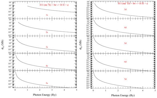
Figure 1.
Photoionization cross sections () of (L) ns and (R) nd levels of hydrogen demonstrating rising trend at threshold and decreasing trend of the background at higher energy with increase of n.
Figure 2 presents of all 5 l-levels (l = 0–4 of shell n = 5. Although all cross sections have the same threshold energy, the peaks at threshold for various levels are different, but the background decays faster with larger l. The bound-free integral in photoionization cross sections depends on the l values as indicating variation with on the angular momentum l. However, it is not linear and hence the general trend can not be predicted. This is demonstrated in Figure 2.
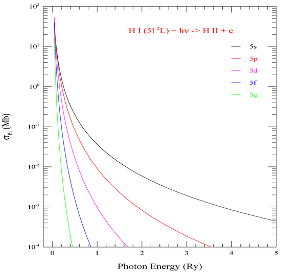
Figure 2.
Photoionization cross sections () of the five l-values (0–4) of shell n = 5. They demonstrate rising trend of for various l-values compared to l = 0 (black curve) at the same ionization threshold.
The program “hpxrrc.f” can be used for of any levels. However, machine accuracy for very low numbers should be discussed. All computations were carried out in double precision using the clusters at Ohio Supercomputer Center (OSC). Numerical instabilities for very small values of at very high n can be summarized as: (i) With increasing energy, cross sections reach to a negligible quantity beyond which computation gives zero value. These cross sections may not add to any significant values. (ii) at threshold continues to dominate while it decreases faster with very high n. (iii) For a very high n, only a few points, sometimes only the threshold value for various l-levels survive before computer prints out zeros even with double precision accuracy. (iv) With a ver high n, such as near n = 700 or 800, even threshold energies become sensitive to the precision of the computer which could yield a lower value. There could be numerical instability in the recurrence relations for these very high n-values in addition to computer numerical tolerence issue. Seaton’s relation without the Gaunt factor or Kramers relation could be useful for such situation of very high-n cross sections.
4.2. Electron-Ion Recombination
The present work reports recombination rates for all individual shells from n = 1 to 800. Some examples are given for demonstration of features.
An example of with n = 10 and l = 0–9 are illustrated in Figure 3. All curves corresponding to l = 0–9 are drawn with different colors and/or with different type (e.g., solid, dashed, or dotted). The sum of all provides the “n-total” curve (red, solid) which is distinctly separated from all curves for individual l-values below it. The figure shows that at low temperature the height of curves do not follow the l-order as expected from l-dependence of at threshold but they follow the order at higher temperature region. of the lowest level does not have the highest peak at lower temperature, but dominates at higher temperature region. The high temperature dominance comes from the slower decrease in of at higher energies compared to the higher l-levels. Couple of small kinks, visible at logarithmic scale, can be noticed for two l-curves (8 and 9) at very high temperature. They arise from some numerical instability of very small values.
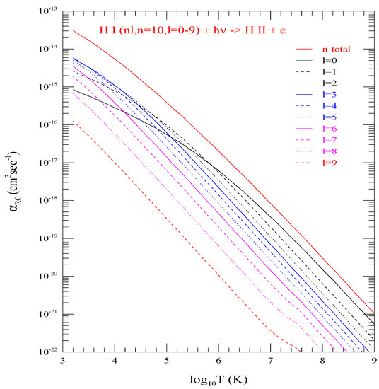
Figure 3.
Level specific electron-ion recombination rate coefficients () of the 10 individual l-levels (0–9) of shell n = 10, and the n-total (red curve with highest values) which is the summed total of all 10 individual levels. They demonstrate peak does not follow values of l-order at low temperature bu follows at higher temperature.
Although for various l-levels belonging to the same n-complex show variations in dominance at lower temperature (Figure 3), the summed total exhibit systematic decrease in values with increasing n. Figure 4 illustrates this behavior with of shells n = 1–10. Various colors/type of curves represent different n as specified in the figure. The topmost curve corresponds to the ground state n = 1 and the lower ones are sequentially in order for n = 2–10. The right panel shows logarithmic behavior of the values. To demonstrate the general linear trend of the values, the left panel presents the linear plot of the same in the same temperature range of to a million degree 10. The curves show sharp rise in at lower temperature for all n = 1–10 with more clarity than in the log-scale.
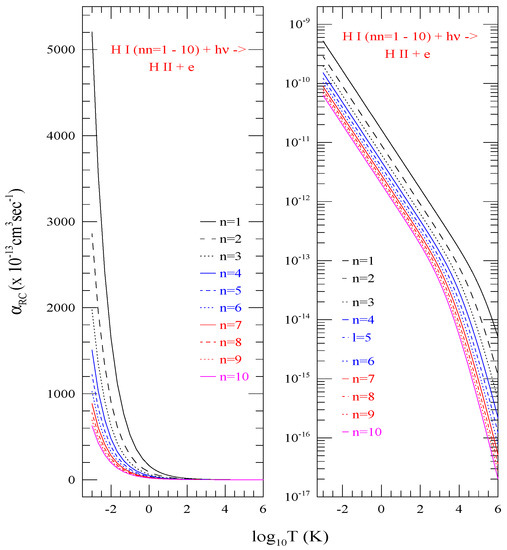
Figure 4.
Total electron-ion recombination rate coefficients () of shells n = 1–10, which are the summed total of all individual l-levels, Left) in linear scale to see the general trend at low temperature and Right) in log scale for logarithmic features. The curves demonstrate decreasing with increasing n.
As mentioned above, the present work provides a file which contains of shells from n = 1 going up n = 800 of hydrogen atom. It does not include components for each n. However, the individual for l-levels which can be computed using the program “hpxrrc.f” as needed.
Figure 5a presents the curve for the total recombination rate coefficients of hydrogen, , which include contributions of individual shells from n = 1 to 800 and the top-up contributions from n = 801 to infinity. Table 1 presents the numerical values of . The range of temperature for is chosen wide, from 10 to 10 K. This allows computation of for hydrogenic ions over a temperature range of practical need. The temperature for an ion of nuclear charge z is equivalent to . Hence, obtaining of a hydrogenic ion of charge z, such as hydrogen-like neon with z = 10, at temperature 1000 K will need at 10 K. As in illustration of calculating of a hydrogenic ion, Figure 5b presents of Fe XXVI obtained from using z-scaling.
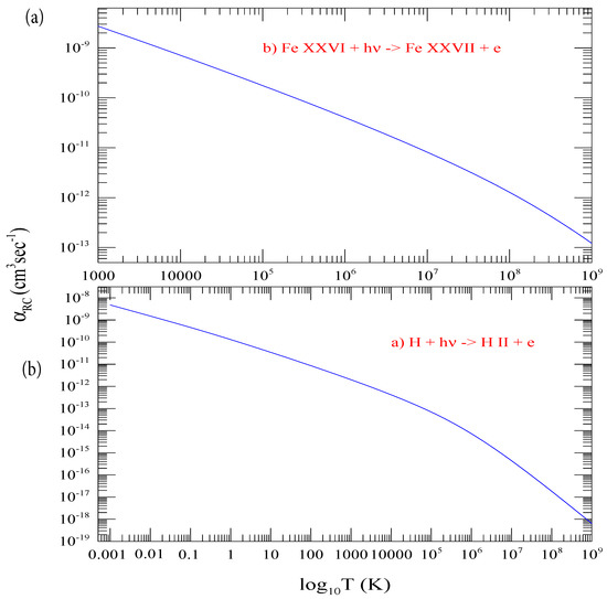
Figure 5.
(a) Total electron-ion recombination rate coefficients , summed contributions from n = 1 to infinity over a wide temperature range. These values are used to obtain (b) of Fe XXVI using the Z-scale formula.

Table 1.
Total recombination rate coefficients of hydrogen, , at a wide range of temperatures.
The total recombination cross sections, , and recombination rate coefficients of hydrogen with respect to the photoelectron energy E are presented in Figure 6. The energy unit is chosen to be in eV because of use of eV unit for the photoelectron in laboratory measurements. Both and include contributions of n = 1–∞. Except for the sharp rise in the very low photoelectron energy, the features show smooth decrease with energy.
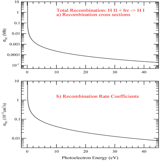
Figure 6.
The total recombination cross sections, , and recombination rate coefficients of hydrogen with respect to the photoelectron energy E.
The present work employs a finite limit integral approach that limits between 0 and 1 replacing the direct dependency on the photoelectron energy going out to infinity. This reduces the uncertainty arising from the limit of energy set for computation of the recombination rate coefficients Hence present results are expected to be most accurate compared to the existing values. The accuracy of the recombination atomic data also depends on the values of photoionization cross sections. As explained in the theory section that the analytical form of has numerical instability which is compensated by the recurrence relations. For very high n. the recurrence relations may have some uncertainties since the cross sections decreases sharply. This may have contributed some uncertaintis in the rates. As explained above that the accuracy of the values also depends on the precision and numerical tolerance of the computer being used. With the best estimation of the factors, that lower-n levels, where values are more stable and accurate, contribute more than the higher-n levels, use of precise theory and numerically stable recurrence relations, and finite limit integration for recombination, the current results are expected to have an accuracy within 5% for most temperature range.
5. Conclusions
The present report can be summarized as
- Study of the two inverse processes of photoionization and electron-ion recombination are presented with a brief review of theory that treat them precisely and more accurately compared to all existing atomic structure codes that use other approximation, mainly distorted wave approximation.
- Detailed features of both the processes are illustrated. Although hydrogen and hydrogenic ions do not have any resonant features, accurate characteristic variation with energy and temperature are crucial for precise astrophysical spectroscopy and modeling.
- The present work provides atomic data files containing for all l-levels of n from 1 to 800, and of all values of n from 1 to 800. It also provides total with temperature, and total , and total with photoelectron energy. This is the first time that all these data with very high n have been made available for applications.
- Use of precise theory, numerical methods, high precision computers, as explained at the end of the sections of photoionization, and electron-ion recombination, can predict the accuracy of the present results is within 5% for most energy and temperature ranges.
- The work provides the FORTRAN program “hpxrrc.f” which can generate all these values. It also computes l-level specific . The program “hpxrrc.f” can also compute for any hydrogenic ion of charge Z using the data of hydrogen.
- Importance of relativistic effects and how to obtain fine structure components for photoionization and electron-ion from their values in the present LS coupling approximation have been discussed.
- All atomic data and the program will be available online at database, NORAD-Atomic-Data ([24], http://norad.astronomy.ohio-state.edu (accessed on 1 September 2007)).
Funding
This research had no external funding. Computations were carried out using computers at the Ohio Supercomputer Center.
Institutional Review Board Statement
Not applicable.
Informed Consent Statement
Not applicable.
Data Availability Statement
All atomic data for photoioization and electron ion recombination, and the program “hpxrrc.f” will be available at NORAD-Atomic-Data: http://norad.astronomy.ohio-state.edu (accessed on 1 September 2007).
Acknowledgments
S.N.N. acknowledges support from the Astronomy Department of the Ohio State University to maintain the database.
Conflicts of Interest
The author declares no conflict of interest. The funder had no role in the design of the study; in the collection, analyses, or interpretation of data; in the writing of the manuscript, or in the decision to publish the results.
References
- Kramers, H.A. XCIII. On the theory of X-ray absorption and of the continuum X-ray spectrum. Lond. Edinb. Dublin Philos. Mag. J. Sci. 1923, 46, 836–871. [Google Scholar] [CrossRef]
- Kotelnikov, I.A.; Milstein, A.I. Electron radiative recombination with ahydrogen-like ion. Phys. Scr. 2019, 94, 055403. [Google Scholar] [CrossRef]
- Rosmej, F.B.; Vainshtein, L.A.; Astapenko, V.A.; Lisitsa, V.S. Statistical and quantum photoionization cross sections in plasmas: Analytical approaches for any configurations including inner shells. Matter Radiat. Extremes 2020, 5, 064202. [Google Scholar] [CrossRef]
- Sugiura, Y.J. Sur le nombre des électrons de dispersion pour les spectres continus et pour les spectres de séries de l’hydrogène. Phys. Radium 1927, 8, 113. [Google Scholar] [CrossRef]
- Gordon, V.W. Zur Berechnung der Matrizen beun Wosserstoff atom. Ann. Phys. 1929, 2, 1031. [Google Scholar] [CrossRef]
- Gaunt, A. Continuous absorption. Philos. Trans. R. Soc. Lond. A 1930, 229, 163. [Google Scholar]
- Menzel, D.H.; Pekeris, C.L. Absorption Coefficients and Hydrogen Line Intensities. Mon. Not. R. Astron. Soc. 1935, 96, 77. [Google Scholar] [CrossRef]
- Bethe, J.A.; Salpeter, E.E. Quantum Mechanics of One- and Two-Electron Atoms; Academics: New York, NY, USA, 1957. [Google Scholar]
- Burgess, A. The Hydrogen Recombination Spectrum. Mon. Not. R. Astron. Soc. 1958, 118, 477. [Google Scholar] [CrossRef]
- Seaton, M.J. Radiative recombination of hydrogenic ions. Mon. Not. R. Astron. Soc. 1959, 119, 81. [Google Scholar] [CrossRef]
- Burgess, A.; Seaton, M.J. A general formula for the calculation of atomic photo-ionization cross sections. Mon. Not. R. Astron. Soc. 1960, 120, 121. [Google Scholar] [CrossRef]
- Burgess, A. Tables of hydrogenic photoionization cross sections and recombination coefficients. Mem. R. Astron. Soc. 1965, 69, 1. [Google Scholar]
- Omidvar, K.; Guimaraes, P.T. New tabulation of the bound-continuum optical oscillator strength in hydrogenic atoms. Astrophys. J. Suppl. 1990, 73, 555–602. [Google Scholar] [CrossRef]
- Green, L.C.; Rush, P.P.; Chandler, C.D. Atomic Transition Prota lities. Astrophys. J. Suppl. 1957, 3, 37. [Google Scholar] [CrossRef]
- Karzas, W.J.; Latter, R. Electron Radiative Transitions in a Coulomb Field. Astrophys. J. Suppl. 1961, 6, 167. [Google Scholar] [CrossRef]
- Ditchburn, R.W.; Öpik, U. Photoionization processes. In Atomic and Molecular Processes; Bates, D.R., Ed.; Academic: New York, NY, USA, 1962; p. 79. [Google Scholar]
- Palenius, H.P.; Kohl, J.L.; Parkinson, W.H. Absolute measurement of the photoionition cross section of atomic hydrogen with a shock tube for the extreme ultraviolet. Phys. Rev. A 1976, 13, 1805. [Google Scholar] [CrossRef]
- Norwood, K.; Ng, C.Y. Photoionization of hydrogen atoms near the ionization threshold. J. Chem. Phys. 1990, 93, 1480. [Google Scholar] [CrossRef]
- Nahar, S.N.; Manson, S.T. Photoionization of the 7d excited state of cesium. Phys. Rev. A 1989, 40, 6300. [Google Scholar] [CrossRef]
- Gu, M.F. The Flexible Atomic Code. AIP Conf. Proc. 2004, 730, 127. [Google Scholar]
- The Opacity Project Team. The Opacity Project; Institute of Physics Publishing: London, UK, 1995; Volume 1, 1996; Volume 2. [Google Scholar]
- TOPbase Website Address for Atomic Database. Available online: http://cdsweb.u-strasbg.fr/topbase/topbase.html (accessed on 1 June 1993).
- Norad. Available online: http://norad.astronomy.ohio-state.edu (accessed on 1 September 2007).
- Nahar, S.N. Database NORAD-Atomic-Data for atomic processes in plasma. Atoms 2020, 8, 68. [Google Scholar] [CrossRef]
- Flower, D.R.; Seaton, M.J. A program to calculate radiative recombination coefficients of hydrogenic ions. Comp. Phys. Commun. 1969, 1, 31. [Google Scholar] [CrossRef]
- Brocklehurst, M. Level populations of hydrogen in gaseous nebulae. Mon. Not. R. Astron. Soc. 1970, 148, 417–434. [Google Scholar] [CrossRef]
- Hummer, D.B.; Storey, P.J. Recombination-line intensities for hydrogenic ions—I. Case B calculations for H I and He II. Mon. Not. R. Astron. Soc. 1987, 224, 801–820. [Google Scholar] [CrossRef]
- Hummer, D.G. Total recombination and energy-loss coefficients for hydrogenic ions at low density for 10 ≤ Te/Z2 ≤ 107 K. Mon. Not. R. Astron. Soc. 1994, 268, 109–112. [Google Scholar] [CrossRef]
- Ferland, G.J.; Peterson, B.M.; Horne, K.; Welsh, W.F.; Nahar, S. Anisotropic line emission and the geometry of the broad-line region in active galactic nuclei. Astrophys. J. 1992, 387, 95. [Google Scholar] [CrossRef]
- Nahar, S.N.; Pradhan, A.K. Electron-ion recombination in the close coupling approximation. Phys. Rev. Lett. 1992, 68, 1488. [Google Scholar] [CrossRef]
- Nahar, S.N.; Pradhan, A.K. Unified Treatment of Electron-Ion Recombination in the Close Coupling Approximation. Phys. Rev. A 1994, 49, 1816. [Google Scholar] [CrossRef]
- Nahar, S.N. Total electron-ion recombination for Fe III. Phys. Rev. A 1996, 53, 2417. [Google Scholar] [CrossRef]
- Nahar, S.N. Electron-ion recombination rate coefficients for Si I, Si II, S II, S III, C II, and C-like ions C I, N II, O III, F IV, Ne V, Na VI, Mg VII, Al VIII, Si IX, and S XI. Astrophys. J. Suppl. 1995, 101, 423, Erratum in 1996, 106, 213. [Google Scholar] [CrossRef]
- Burke, P.G. Photoionization of atomic systems. In Atomic Processes and Applications: In Honour of David R. Bates’ 60th Birthday; Burke, P.G., Moiseiwitsch, B.L., Eds.; North-Holland Publishing: Amsterdam, The Netherlands, 1976; pp. 199–248. [Google Scholar]
- Kogan, V.I.; Kukushkin, A.B.; Lisitsa, V.S. Kramers Electrodynamics and electron—Atomic radiative—Collisional processes. Phys. Rep. 1992, 213, 1–116. [Google Scholar] [CrossRef]
- Pradhan, A.K.; Nahar, S.N. Atomic Astrophysics and Spectroscopy; Cambridge University Press: New York, NY, USA, 2011. [Google Scholar]
- Biedenharn, L.C.; McHale, J.L.; Thaler, R.M. Quantum calculation of Coulomb excitation. I. Phys. Rev. 1955, 100, 376. [Google Scholar] [CrossRef]
- Alder, K.; Winther, A.K. On the Exact Evaluation of the Coulomb Excitation. Det Kongelge Dankske Videnskabernes Selskab. Mat.-Fys. Medd. 1955, 29, 19. [Google Scholar]
- Sommefeld, A. Atombau und Spektrallinien: Band I und II; Harri Deutsch: Frankfurt, Germany, 1978. [Google Scholar]
- Krainov, V.; Reiss, H.R.; Smirnov, B.M. Radiative Processes in Atomic Physics; John Wiley and Sons Inc.: New York, NY, USA, 1997. [Google Scholar]
- Samson, A.R. The measurement of the photoionization cross sections of the atomic gases. Adv. At. Mol. Phys. 1966, 2, 237. [Google Scholar]
- Zhang, H.L.; Nahar, S.N.; Pradhan, A.K. Close coupling R-matrix calculations for electron-ion recombination cross sections. J. Phys. B 1999, 32, 1459. [Google Scholar] [CrossRef]
- Pradhan, A.K.; Nahar, S.N.; Zhang, H.L. Unified electronic recombination of ne-like fe xvii: Implications for modeling X-ray plasmas. Astrophys. J. Lett. 2001, 549, L265. [Google Scholar] [CrossRef]
- Nahar, S.N. Atomic Data from the IRON Project VII. Radiative Dipole Transition Probabilities for Fe II. Astron. Astrophys. 1995, 293, 967. [Google Scholar]


Publisher’s Note: MDPI stays neutral with regard to jurisdictional claims in published maps and institutional affiliations. |
© 2021 by the author. Licensee MDPI, Basel, Switzerland. This article is an open access article distributed under the terms and conditions of the Creative Commons Attribution (CC BY) license (https://creativecommons.org/licenses/by/4.0/).