Abstract
A Sagnac atom interferometer can be constructed using a Bose–Einstein condensate trapped in a cylindrically symmetric harmonic potential. Using the Bragg interaction with a set of laser beams, the atoms can be launched into circular orbits, with two counterpropagating interferometers allowing many sources of common-mode noise to be excluded. In a perfectly symmetric and harmonic potential, the interferometer output would depend only on the rotation rate of the apparatus. However, deviations from the ideal case can lead to spurious phase shifts. These phase shifts have been theoretically analyzed for anharmonic perturbations up to quartic in the confining potential, as well as angular deviations of the laser beams, timing deviations of the laser pulses, and motional excitations of the initial condensate. Analytical and numerical results show the leading effects of the perturbations to be second order. The scaling of the phase shifts with the number of orbits and the trap axial frequency ratio are determined. The results indicate that sensitive parameters should be controlled at the level to accommodate a rotation sensing accuracy of rad/s. The leading-order perturbations are suppressed in the case of perfect cylindrical symmetry, even in the presence of anharmonicity and other errors. An experimental measurement of one of the perturbation terms is presented.
1. Introduction
Atom interferometry is useful for many types of precision measurements [1,2,3], but one of the most attractive applications is inertial navigation [4,5]. For this purpose, atom interferometers can be configured to measure accelerations [6,7], rotations [8,9], or both simultaneously [10,11]. In order to obtain high sensitivity, it is desirable to operate the interferometer with long measurement times T. This can be a challenge for measurements with freely falling atoms, since a large fall distance will increase the apparatus size and complexity. One solution is to support the atoms against gravity using a magnetic field [12]. This unavoidably leads to some confinement as well [13], but we can make use of this confining potential to help guide the atoms along a desired trajectory.
In Ref. [14], we demonstrated a Sagnac interferometer using atoms confined in a harmonic potential, where the trap caused the atoms to move in nearly circular orbits so as to enclose an area. By using two simultaneous counter-propagating interferometers in the same trap, many spurious phase shifts can be rejected through a differential measurement. However, if the confining potential is not ideal then it can still impact the final phase measurement and limit the accuracy of the sensor. In this paper, we analyze the phase shifts imparted by the potential and present the dependence on various perturbative terms. We find that it is possible to reach performance levels consistent with precision navigation requirements, but that doing so will require precise control of the trapping parameters.
The analysis described here is similar to that by West in Ref. [15]. However, in that work only a single interferometer was considered. By design, many errors cancel in the dual-interferometer scheme of [14], making our approach mainly sensitive to higher-order effects that were not comprehensively addressed in [15]. In addition, our numerical analysis considers a wider variety of perturbative parameters, including ones that couple all three dimensions.
The analysis here focuses exclusively on the phase shifts induced by the perturbations. The interferometer visibility and enclosed area are also impacted by non-idealities. These are not affected by the differential measurement, so the analysis in [15] is directly applicable. While the visibility and area are important, we expect the phase to be the most sensitive parameter, so if perturbations are reduced to the point that phase shifts are negligible, the visibility and area will also be close to ideal.
In the following, we first present our interferometer scheme and the semiclassical approach we use for the analysis. We apply the approach analytically to the case of a harmonic trapping potential with a limited number of perturbations. We then present numerical results for a broader set of perturbations. Finally, we discuss the implications for experiments and compare to a measurement of the phase sensitivity for one pair of parameters.
2. Semiclassical Phase Analysis
The atom trajectories used in our interferometer scheme are illustrated in Figure 1. A Bose condensate is first prepared nominally at rest in the center of an approximately harmonic trap. We define a coordinate system centered on the trap, with z vertical. An off-resonant standing wave laser is applied along the y direction, driving the atoms into a superposition of states moving at momenta , where k is the wave number of the laser [16]. The two wave packets separate, and after one quarter of an oscillation period they come to rest on opposite side of the trap. At that time another standing wave is applied along the x direction, resulting in a total of four wave packets. The momentum kicks along x cause each packet to move in a nearly circular orbit around the center of the trap. The packets are sufficiently dilute that they can pass through each other with negligible losses. After one or more orbits, the x standing wave is applied again, closing each of the two interferometers. If the quantum state of two packets prior to the recombination pulse is
then the probability for an atom to be brought to rest by the recombination pulse is for phase difference ; atoms not brought to rest continue moving. After a short time of flight, the atoms can be imaged and the fraction of the population in each momentum state can be determined.
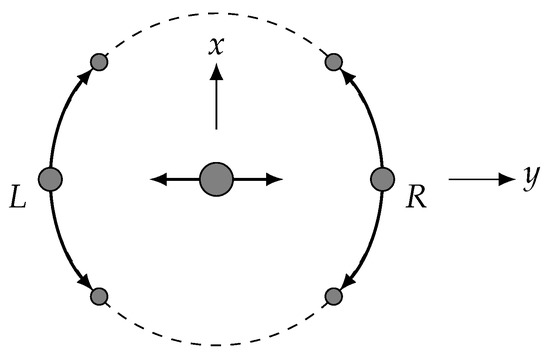
Figure 1.
Trajectory of atoms in Sagnac interferometer. A condensate, represented by gray disks, starts in the center of the harmonic trap at time . A standing-wave laser oriented along y splits the condensate into two packets that move in the directions. One quarter period later, the atoms come to rest on the left (L) and right (R) sides of the trap. Another standing-wave laser oriented along x then splits the atoms again. The resulting packets have the correct velocity to travel in a circular orbit around the trap center. After n complete orbits, the x-laser is applied again. This brings some of the moving atoms back to rest on their respective sides of the trap. The fraction brought to rest depends on the phase difference between the two interfering packets.
One contribution to the phase is the Sagnac effect, giving where A is the area enclosed by an orbit, m is the atomic mass, and is the rotation rate of the apparatus. This phase applies with opposite signs to the two interferometers, so if denotes the phase measured at positive y and denotes the phase measured at negative y, we have . This is the signal used for rotation sensing.
Our goal in this paper is to analyze other contributions to this differential phase, so we assume . The remaining phase for a single interferometer is given in the semiclassical approximation by a sum of three terms [17]:
The first is the dynamical phase acquired by the atoms as they move through the trap. Each packet acquires a phase , for Lagrangian evaluated on the classical trajectory of the packet. Here is the trapping potential. We therefore express
where the x-splitting pulse is applied at time and the recombination pulse at time . The ± labels refer to the wave packet that initially received a Bragg kick in the direction, with indicating the Lagrangian evaluated along that packet’s trajectory.
The laser phase is set by the location of the atoms relative to the Bragg standing wave. If the atoms are initially split at position and recombined at position , then the interferometer registers a phase shift
An additional phase shift will appear if the position of the Bragg standing wave itself changes between the two pulses, but we omit this effect since the additional shift will be the same for both interferometers and thus cancel in . If the interferometer is not closed, such that the final positions of the packets are and , then we evaluate the phase at the center position .
The separation phase also arises when the interferometer is not closed, and it accounts for the fact that if the final packets are not at rest, their phases are themselves position-dependent. This results in
where are the final wave packet velocities.
For a single atom in a harmonic potential, the semiclassical approximation is very accurate since it agrees with the fully quantum results obtained using coherent-state wave functions. However, interacting atoms in a condensate will occupy a Thomas–Fermi wave function which can be quite different from a coherent state [18]. In addition, the wave function can be distorted by anharmonic perturbations. These effects are not accounted for in the semiclassical approach. We are currently exploring this issue using an approach based on the Gross–Pitaevskii equation for an interacting condensate [19,20]. Preliminary results indicate that the semiclassical approximation is still quite accurate as long as the anharmonic perturbations are small. Use of a realistic wave function might, however, have more significant impact on the visibility and effective enclosed area.
3. Harmonic Oscillator Potential
For a harmonic trap, the classical trajectories can be expressed analytically, which allows an analytic calculation of the final differential phase . We consider a potential of the form
Here the are the principal coordinates of the trap, in which the potential has this diagonal form. The are the corresponding oscillation frequencies. The principal coordinates do not in general conform to the coordinates by which the Bragg laser beams are defined as in the previous section. We work in the principal coordinates and take the Bragg wave vectors as
for principal basis vectors and unit vector components .
If at time an atom has position and velocity , its subsequent trajectory is given by
and
Since the Lagrangian is separable in the principal coordinates, the dynamical phase can be calculated for each coordinate independently, and can be evaluated as
To apply this result, we must express the trajectory in our interferometer. We suppose the initial condensate has position and velocity . The y Bragg laser is applied at time zero, and the atoms are allowed to propagate for time . The wave packets then have coordinates
where is the velocity kick from the Bragg beam. We take for atoms kicked in the directions. To help keep the notation clear, we label with R and with L. The starting velocities for the actual interferometers also include the x-Bragg kicks, leading to trajectories
Here we use the + and − symbols to label the sign of the kicks received from the x beams. The atoms orbit for a time , so the total duration of the motion is .
We use these trajectories to evaluate the phase. We set as the dynamical differential phase and find
The separation phase of Equation (5) can be evaluated in terms of the final positions and velocities. We obtain
so this term exactly cancels the dynamical phase here. The net differential phase is therefore given by , which is evaluated to be
The ideal case consists of a cylindrically symmetric trap with in the horizontal directions, and perhaps different in the vertical direction. The Bragg beams should have , with the other components equal to zero. We then obtain and there is no phase shift from the trap potential. To allow for small deviations from the ideal case, we consider a nearly-symmetric potential of the form
with and small compared to one. This can be diagonalized to give principal horizontal frequencies
where . We take to use the plus sign and to use the minus sign. The principal directions can then be expressed
We also allow the Bragg beams to deviate slightly from their nominal alignments, with
for . Finally, we allow for timing errors, defining
for an interferometer with n orbits.
We then expand the total phase to second order in the small parameters. We obtain
Note that the radius of the orbit which the atoms undergo is , so the prefactors scale as , which is very large for orbits of mm or cm size. We see that the critical parameters are the timing, the term in the potential, and the vertical alignment of the Bragg beams. There is no first-order dependence on small parameters.
4. Anharmonic Potential
More generally, the trapping potential will not be perfectly harmonic, so it is important to understand the impact of small anharmonic terms. Anharmonic perturbations make analytical calculations complicated [21], so here we use a numerical approach. We consider a trapping potential of the form
with the coefficients dimensionless and small compared to 1. We include corrections from second to fourth order, , noting that first-order terms can always be eliminated by offsetting the location of the trap minimum.
Other perturbative parameters are the initial position , the initial velocity , the Bragg alignment errors from Equations (19) and (20), and the timing errors , . Because the perturbations can change the effective oscillation frequency, we here determine numerically the nominal values for and . For , we set as the time when the separation between the right and left wave packets is maximized. We then set . For , we set as the time at which the distance between the two interfering wave packets is a minimum, after making n orbits around the trap. Specifically, we minimize the quantity
where the positions are labeled as in Equation (12). We then set . This procedure mimics the way the timing would be determined experimentally. In total, we include forty-three perturbation parameters in the analysis, all of which are dimensionless.
The classical trajectories themselves are determined using the MATLAB ode45 solver, with tolerance parameters of . The solver is simultaneously used to integrate the dynamic phase terms of Equation (3). The initial and final points of the trajectories are used to determine and via Equations (4) and (5). From these, the total differential phase is calculated. We then vary the expansion parameters to determine their sensitivity. We numerically calculate both the first derivatives and second derivatives for expansion parameters . We use an increment step and we estimate the derivative values to have a numerical accuracy of or better.
We first consider the case of a spherically symmetric potential with in Equation (23). We observe no first-order dependence on the expansion parameters, but we observe thirty significant second-order terms, displayed in Table 1. Although these are numerical results, we find they reduce to simple fractions when appropriate factors of are included. We determined the n dependence by fitting the results to low-order polynomials, again obtaining simple integer coefficients. The terms listed in the table are all those with magnitudes larger than at . The dependence on , and agrees with the analytic results from Equation (22). We observe dependencies on and , corresponding to and in Equation (16), which are not present in Equation (22); this arises due to the difference in how and are treated. Of the forty-three parameters considered, we find that sixteen contribute to second-order terms.

Table 1.
Sensitivity of the differential phase to small parameters . The phase is normalized by for Bragg laser wave number k and nominal orbit radius R. The integer number of orbits is n. Here we show the thirty significant terms observed for a spherically symmetric trap with . The entries below the horizontal line in the second column depend on , as seen in Table 2.
We also consider the case of a cylindrically symmetric trap, with . Most of the terms reported in Table 1 are unchanged, so Table 2 reports only those which are different. Terms in the first column and above the line in the second column do not appear in Table 1. Terms below the line are those from from Table 1 that are observed to depend on . Here we map out the dependence on both n and by calculating a range of values and guessing appropriate fitting functions; again we find simple numerical coefficients. An example of this analysis is described in Figure 2. We find that the term involving and agrees with the analytic result of (22). Note that although the terms in the table exhibit poles in , the divergences are all canceled by zeros of the functions. We confirmed that the limits for agree with the values in Table 1. As before, the table includes all terms with magnitudes larger than at . Here we find an additional seven parameters contributing to the phase.
Table 2.
Phase sensitivity for a cylindrically symmetric trap with . Terms below the horizontal line in the second column are those that that differ from their values in the spherically symmetric case of Table 1. Other terms from Table 1 apply without change. Terms in the first column and above the line are those that appear only in the cylindrical case. The dependence on and on the number of orbits n are determined numerically. The n-dependence is parametrized by the functions , , and .
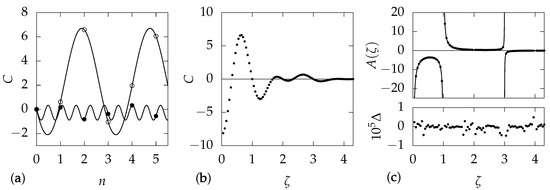
Figure 2.
Analysis of numerical results, for the example term with and . (a) Variation of C with orbit number n. The open points show results for , and the filled points for . From the analytical results, we anticipate that the phase will vary sinusoidally with , and we also know that at . We therefore fit the points to a function , with the results shown as curves. While the amplitude A depends on , we obtain in all cases. (b) Variation of C with , for . This illustrates that the result is a smooth function over the range considered. (c) Points in the upper plot show the variation with of the amplitude . The graph exhibits obvious poles at , , and . We incorporate these polls into a rational fit function and find good agreement for constant . The curves show this fit. In the lower plot, is the fit residual . At larger , the residuals grow but the coefficient C is very small.
The total of twenty-three parameters that contribute in second order fall into two independent groups, with no phase terms drawing from both groups. The terms above the line in Table 1 depend on ten parameters that characterize the horizontal motion only. The remaining thirteen parameters involve coupling to the vertical motion. Of this second group, six contribute when , but only three, and , contribute when . None contribute when or a larger integer. Reducing the number of sensitive parameters is useful since it makes the rotation sensor more robust.
It is interesting to consider which perturbation terms would be present in a trap that maintained perfect cylindrical symmetry. This symmetry requires , , , and ; other potential terms involving x and y must be zero. In this case, the only surviving second-order term is the dependence from Table 2, which can itself be eliminated if is close to an integer. Using these symmetry constraints to reduce the parameter space, we also explored the third-order dependence of . Table 3 lists the twelve largest terms observed, in the case . Here the largest omitted term has a magnitude (at ) that is nine times smaller than the smallest term included. From the results, it is evident that the horizontal quartic anharmonicity is particularly important at this order.
Table 3.
Third-order sensitivities in the case of a trap with perfect cylindrical symmetry, for n orbits with .
5. Implications for Experiments
Phase shifts arising from imperfections in the trapping potential will limit the accuracy of the interferometer’s performance as a rotation sensor. If we interpret a second-order perturbation from the potential as a rotation error , then we evaluate the corresponding Sagnac phase as
where is an entry from Table 1 or Table 2. Using , we have
The largest coefficients C have magnitudes that are comparable to , so we conclude that the effective rotation error is approximately . This indicates the level of trap imperfections that can be tolerated for a given rotation accuracy. For instance, achieving an accuracy of order rad/s in a trap with Hz and would require the to be of order . This result also indicates that the sensitivity to trap imperfections generally increases with n and , so it is better to use a single orbit in a weaker trap, as opposed to multiple orbits in a tighter trap to achieve the same Sagnac area.
It is experimentally feasible to implement a magnetic trap that is stable to a part in or better [22,23], but it would be challenging to design a trap with imperfections that are zero to this level of accuracy. One approach would be to accept a static phase offset that can be measured and subtracted out to obtain a pure rotation signal, but the stability tolerance required for a parameter grows more stringent the larger its partner parameter is. Alternatively, if all relevant trap parameters can be adjusted experimentally, the interferometer itself can be used to set the parameters to zero. The second-order phase error is
where here is a vector of experimental parameters and contains the (initially unknown) parameter values for which the interferometer configuration is ideal. The matrix M is composed of second derivatives , which can either be calculated as in the previous sections or measured experimentally by varying the parameters in pairs and observing the phase response. In a similar way, the gradient vector can be measured experimentally at an initial value of . Since , we can obtain an estimate for as
The parameters can then be set to this and the process can be iterated to converge on the desired parameter set where . To this end, it is useful that the parameters fall into independent groups, since this means each group can be optimized independently.
We have experimentally demonstrated the required measurement procedure using the apparatus of Ref. [14]. Here we focus on two parameters, the timing error and the potential term . Experimental control of is straightforward via timing. To control , we make use of a feature of the time-orbiting potential trap. Our trap uses a rotating bias field with components
where kHz, , and is an experimentally adjustable phase. In combination with an oscillating gradient field and gravity, this produces a time-averaged potential [14,24]
where the phase provides the desired control of the term. Comparing to Equation (22), we see . The experiment used Rb atoms in a trap with Hz. The Bragg wave number was .
The interferometer was operated as in Ref. [14], with no imposed rotation. For set values of and , the output differential phase was determined by taking several measurements of the two interferometer signals and , with defined as the fraction of atoms returned to rest in interferometer s. As seen in Figure 3a insets, the data fall on ellipses when is plotted against . The location of a point on the ellipse is determined by the common mode phase of the two interferometers, which is noisy in our experiment. The ellipticity e depends on the differential phase as , so the phase can be extracted by fitting the data to an ellipse.
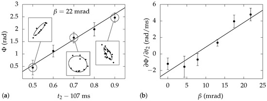
Figure 3.
Experimental measurement of phase sensitivity. (a) Variation of differential phase with interferometer time . Results are for a trap with magnetic field phase mrad. The line is a linear fit from which the slope is determined. Insets show plots of vs. at the indicated values of . The curves are elliptical fits from which the phase values are determined. (b) Slopes from (a) plotted vs. . The line is again a linear fit with slope s.
Using this technique, we measured the dependence of on , and found a linear variation as seen in Figure 3a. We fit these data to determine the slope , and repeated the measurements over a range of bias field phases . Figure 3b shows that itself varies linearly with , so from the slope in Figure 3b we determine rad/s. This corresponds to
In comparison, Equation (22) predicts for that . The measurement and calculation differ by , which is ambiguous in terms of agreement. We are currently developing a new apparatus that will substantially improve the measurement precision and allow a more definitive test of the model.
If and were the only trap imperfections to consider, then it would be possible to establish the experimental settings where both parameters were zero, as the point where . However, Table 1 indicates that and are also coupled to and the horizontal quartic anharmonicities. Since these variables have not been considered, we cannot expect that when here.
We do have some information about the trap anharmonicity. As described in Ref. [25], the potential can be characterized using the observed packet trajectories. Using mm, we find , , , and . Although these terms are not very small, the numerical model predicts that they do not significantly change the expected value of determined above.
6. Conclusions
The methods presented here are generally useful for characterizing the performance of a trapped atom interferometer. The results for our Sagnac interferometer scheme show which experimental imperfections are most critical, and they provide guidance for how well they must be controlled in order to reach a desired level of rotation sensitivity. It is promising that the system is primarily sensitive to parameters that break the cylindrical symmetry, since these parameters will be naturally small in an experimental design which is nominally symmetric. Nonetheless, the parameters will need to be be controlled very precisely to reach state-of-the-art performance levels.
It may also be possible to develop operational protocols which help reduce the sensitivity to imperfections. For instance, the interferometer can instead be operated by splitting first along x and then along y. This would alter many of the trap phase terms but not the Sagnac phase, so comparing the two results could reduce the sensitivity to perturbations. We hope to explore this and other schemes in future work.
Author Contributions
Conceptualization, C.A.S.; methodology, Z.L., E.R.M. and C.A.S.; software, Z.L. and C.A.S.; validation, Z.L., E.R.M. and C.A.S.; formal analysis, Z.L., E.R.M. and C.A.S.; investigation, Z.L, E.R.M. and C.A.S.; writing—original draft preparation, C.A.S.; writing—review and editing, Z.L. and E.R.M.; visualization, E.R.M. and C.A.S.; supervision, C.A.S.; project administration, C.A.S.; funding acquisition, C.A.S. All authors have read and agreed to the published version of the manuscript.
Funding
This research was funded by the Defense Advanced Research Projects Agency grant number FA9453-19-1-0007, National Science Foundation grant number PHY-1607571 and NASA grant number RSA1549080g.
Institutional Review Board Statement
Not applicable.
Informed Consent Statement
Not applicable.
Data Availability Statement
The data presented in this study are openly available from OSF at doi:10.17605/OSF.IO/HAU9W.
Acknowledgments
We are pleased to acknowledge advice and comments on the manuscript from M. Edwards and J. Stickney, and we acknowledge assistance with the experimental measurements from A. Fallon and S. Berl.
Conflicts of Interest
The authors declare no conflict of interest.
References
- Berman, P.R. (Ed.) Atom Interferometry; Academic Press: San Diego, CA, USA, 1997. [Google Scholar]
- Cronin, A.D.; Schmiedmayer, J.; Pritchard, D.E. Optics and interferometry with atoms and molecules. Rev. Mod. Phys. 2009, 81, 1051. [Google Scholar] [CrossRef]
- Tino, G.M.; Kasevich, M.A. (Eds.) Atom Interferometry; Proceedings of the International School of Physics “Enrico Fermi” Series; IOS Press: Amsterdam, The Netherlands, 2014; Volume 188. [Google Scholar]
- Grewal, M.S.; Andrews, A.P.; Bartone, C.G. Global Navigation Satellite Systems, Inertial Navigation, and Integration, 3rd ed.; Wiley: Hoboken, NJ, USA, 2013. [Google Scholar]
- Geiger, R.; Landragin, A.; Merlet, S.; Dos Santos, F.P. High-accuracy inertial measurements with cold-atom sensors. AVS Quantum Sci. 2020, 2, 024702. [Google Scholar] [CrossRef]
- McGuirk, J.; Foster, G.; Fixler, J.; Snadden, M.; Kasevich, M. Sensitive absolute-gravity gradiometry using atom interferometry. Phys. Rev. A 2002, 65, 033608. [Google Scholar] [CrossRef]
- Schmidt, M.; Senger, A.; Hauth, M.; Freier, C.; Schkolnik, V.; Peters, A. A mobile high-precision absolute gravimeter based on atom interferometry. Gyroscopy Navig. 2011, 2, 170. [Google Scholar] [CrossRef]
- Durfee, D.S.; Shaham, Y.K.; Kasevich, M.A. Long-term stability of an area-reversible atom-interferometer Sagnac gyrosope. Phys. Rev. Lett. 2006, 97, 240801. [Google Scholar] [CrossRef] [PubMed]
- Savoie, D.; Altorio, M.; Fang, B.; Sidorenkov, L.A.; Geiger, R.; Landragin, A. Interleaved atom interferometry for high-sensitivity inertial measurements. Sci. Adv. 2018, 4. [Google Scholar] [CrossRef] [PubMed]
- Dickerson, S.M.; Hogan, J.M.; Sugarbaker, A.; Johnson, D.M.S.; Kasevich, M.A. Multiaxis inertial sensing with long-time point source atom interferometry. Phys. Rev. Lett. 2013, 111, 083001. [Google Scholar] [CrossRef] [PubMed]
- Chen, Y.J.; Hansen, A.; Hoth, G.W.; Ivanov, E.; Pelle, B.; Kitching, J.; Donley, E.A. Single-source multiaxis cold-atom interferometer in a centimeter-scale cell. Phys. Rev. Appl. 2019, 12, 014019. [Google Scholar] [CrossRef]
- Garrido Alzar, C.L. Compact chip-scale guided cold atom gyrometers for inertial navigation: Enabling technologies and design study. AVS Quatnum Sci. 2019, 1, 014702. [Google Scholar] [CrossRef]
- Sackett, C.A. Limits on weak magnetic confinement of neutral atoms. Phys. Rev. A 2006, 73, 013626. [Google Scholar] [CrossRef]
- Moan, E.R.; Horne, R.A.; Arpornthip, T.; Luo, Z.; Fallon, A.J.; Berl, S.J.; Sackett, C.A. Quantum rotation sensing with dual Sagnac interferometers in an atom-optical waveguide. Phys. Rev. Lett. 2020, 124, 120403. [Google Scholar] [CrossRef] [PubMed]
- West, A.D. Systematic effects in two-dimensional trapped matter-wave interferometers. Phys. Rev. A 2019, 100, 063622. [Google Scholar] [CrossRef]
- Wu, S.; Wang, Y.; Diot, Q.; Prentiss, M. Splitting matter waves using an optimized standing-wave light-pulse sequence. Phys. Rev. A 2005, 71, 043602. [Google Scholar] [CrossRef]
- Hogan, J.M.; Johnson, D.M.S.; Kasevich, M.A. Light-pulse atom interferometry. In Atom Optics and Space Physics; Proceedings of the International School of Physics “Enrico Fermi” Series; Arimondo, E., Ertmer, W., Schleich, W.P., Rasel, E., Eds.; IOS Press: Amsterdam, The Netherlands, 2009; Volume 168, pp. 411–447. [Google Scholar]
- Dalfovo, F.; Giorgini, S.; Pitaevskii, L.; Stringari, S. Theory of Bose–Einstein condensation in trapped gases. Rev. Mod. Phys. 1999, 71, 463. [Google Scholar] [CrossRef]
- Edwards, M.; Henry, C.; Thomas, S.; Sapp, C.; Clark, C. Precision Gross–Pitaevskii modeling of a dual-Sagnac interferometer. In Bulletin of the American Physical Society, Proceedings of the 51st Annual Meeting of the APS Division of Atomic, Molecular and Optical Physics, Virtual Conference, 1–5 June 2020; American Physical Society: College Park, MD, USA, 2020; Volume 56, p. 56. [Google Scholar]
- Stickney, J. (Space Dynamics Laboratory, North Logan, UT, USA). Personal communication, 2020.
- Landau, L.D.; Lifschitz, E.M. Mechanics, 3rd ed.; Pergammon Press: Oxford, UK, 1976. [Google Scholar]
- Merkel, B.; Thirumalai, K.; Tarlton, J.E.; Schäfer, V.M.; Ballance, C.J.; Harty, T.P.; Lucas, D.M. Magnetic field stabilization system for atomic physics experiments. Rev. Sci. Instrum. 2019, 90, 044702. [Google Scholar] [CrossRef] [PubMed]
- Xu, X.T.; Wang, Z.Y.; Jiao, R.H.; Yi, C.R.; Sun, W.; Chen, S. Ultra-low noise magnetic field for quantum gases. Rev. Sci. Instrum. 2019, 90, 054708. [Google Scholar] [CrossRef] [PubMed]
- Moan, E.R. Rotation Sensing Using Atom Interferometry in a Magnetic Trap. Ph.D. Thesis, University of Virginia, Charlottesville, Virginia, 2020. [Google Scholar]
- Moan, E.; Berl, S.; Luo, Z.; Sackett, C.A. Controlling the anharmonicity of a time-orbiting potential trap. In Optical, Opto-Atomic, and Entanglement-Enhanced Precision Metrology II; Shahriar, S., Scheuer, J., Eds.; SPIE: Bellingham, WA, USA, 2020; Volume 11296. [Google Scholar] [CrossRef]


Publisher’s Note: MDPI stays neutral with regard to jurisdictional claims in published maps and institutional affiliations. |
© 2021 by the authors. Licensee MDPI, Basel, Switzerland. This article is an open access article distributed under the terms and conditions of the Creative Commons Attribution (CC BY) license (http://creativecommons.org/licenses/by/4.0/).