New Energy Levels and Transitions of 5s25p2 (6d+7s) Configurations in Xe IV


Abstract
1. Introduction
2. Experimental Methods
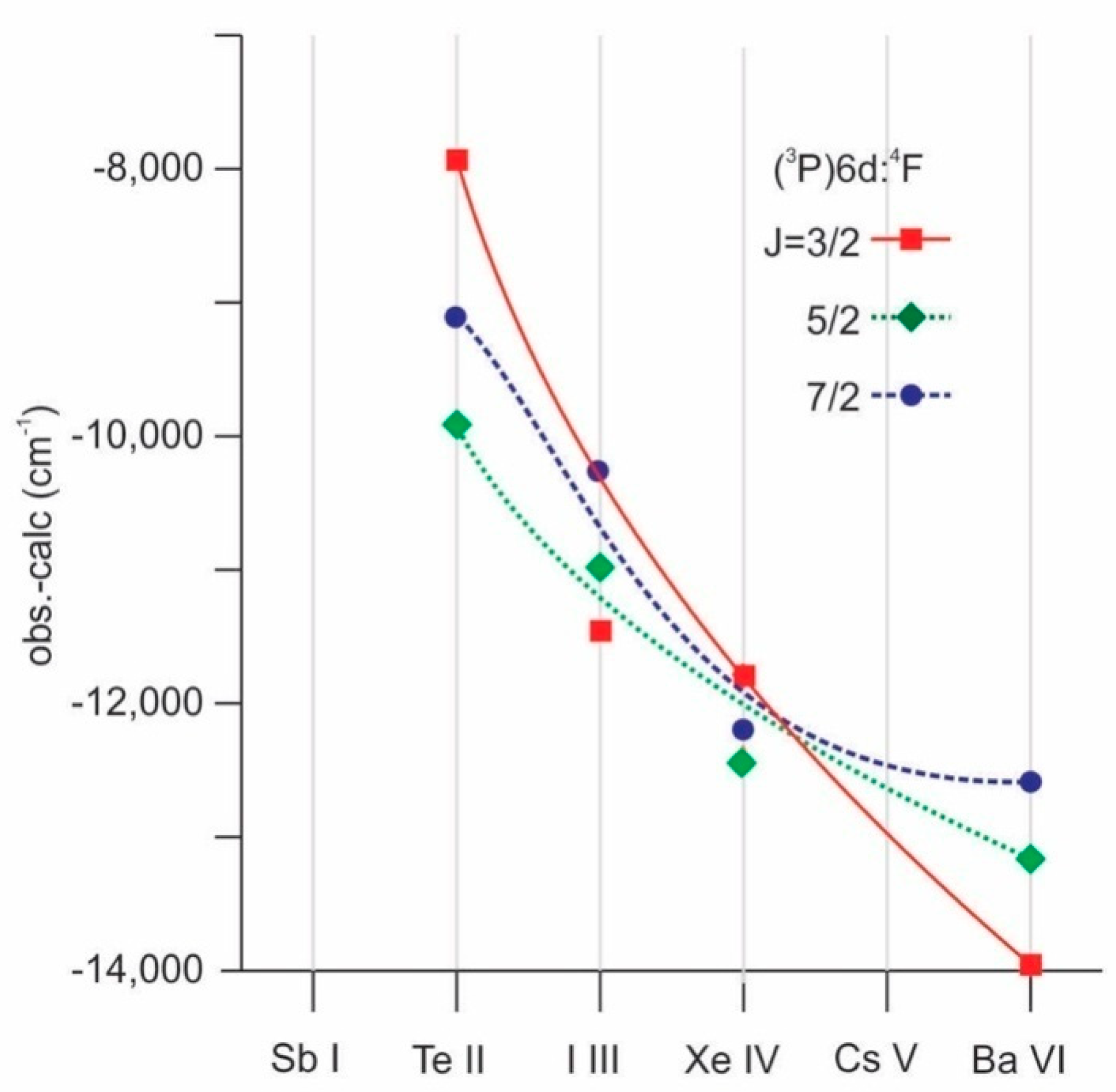
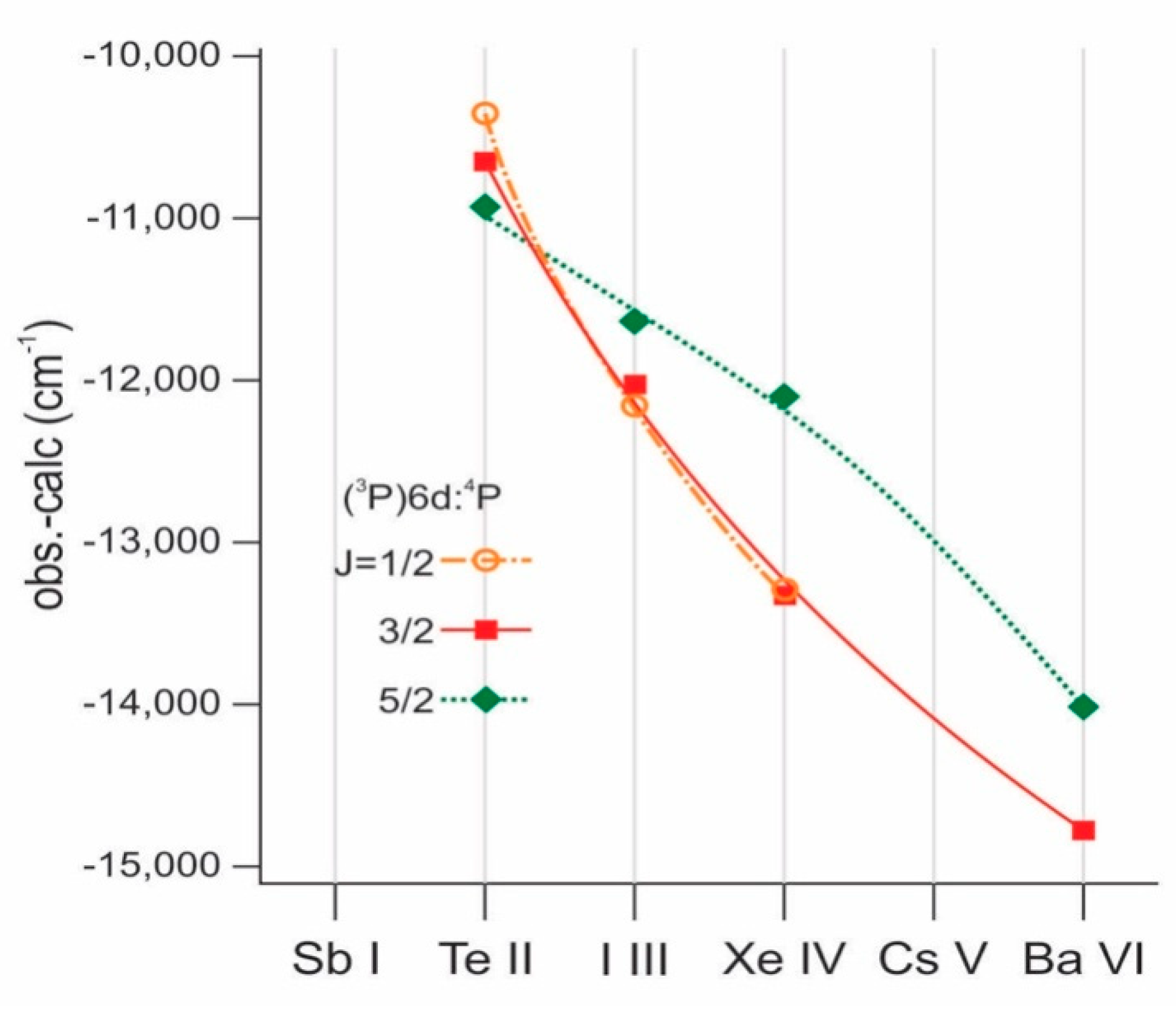
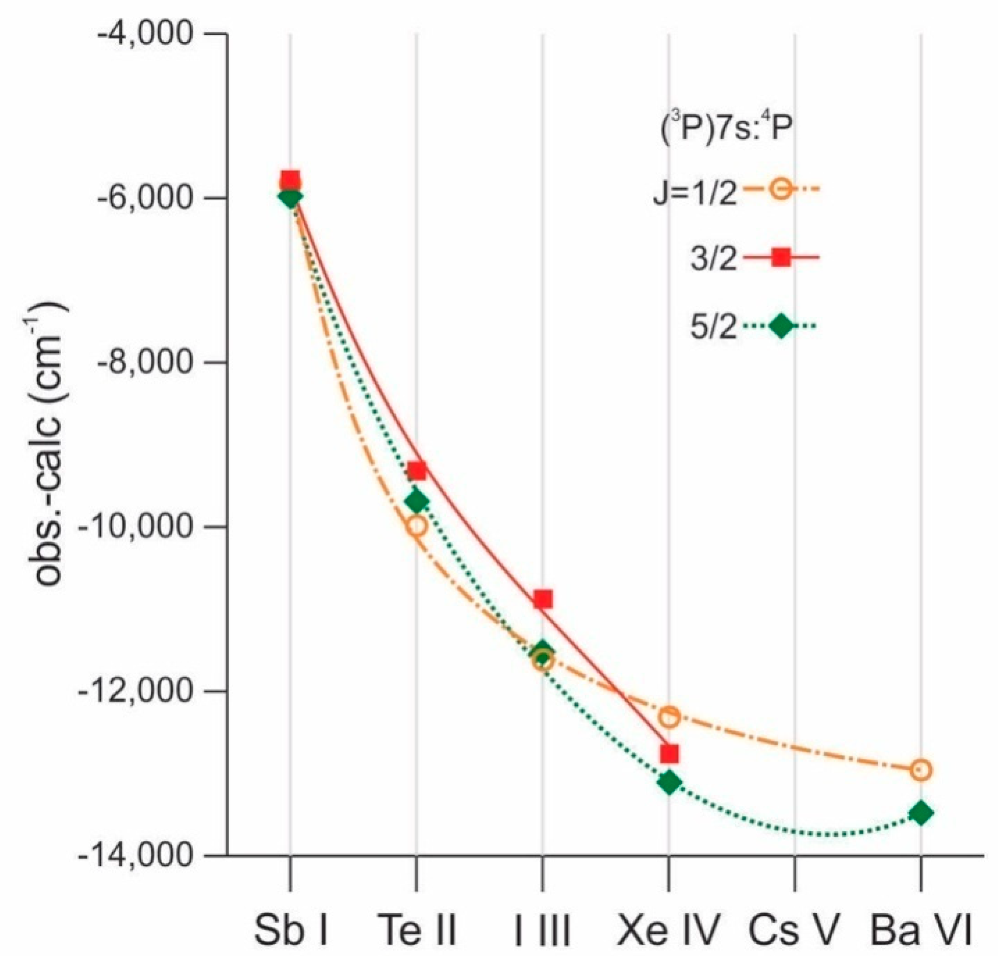
3. Results and Discussion
4. Conclusions
Author Contributions
Funding
Acknowledgments
Conflicts of Interest
References
- Gustafsson, B. The future of stellar spectroscopy and its dependence on YOU. Phys. Scr. 1991, 34, 14–19. [Google Scholar] [CrossRef]
- Biémont, E.; Blagoev, K.; Campos, J.; Mayo, R.; Malcheva, G.; Ortíz, M.; Quinet, P. Radiative parameters for some transitions in Cu(II) and Ag(II) spectrum. Spectrosc. Relat. Phenom. 2005, 144, 27–28. [Google Scholar] [CrossRef]
- Cowley, C.R.; Hubrig, S.; Palmeri, P.; Quinet, P.; Biémont, É.; Wahlgren, G.M.; Schütz, O.; González, J.F. HD 65949: Rosetta stone or red herring. Mon. Not. R. Astron. Soc. 2010, 405, 1271–1284. [Google Scholar] [CrossRef]
- Otsuka, M.; Tajitsu, A. Chemical abundances in the extremely carbon-rich and xenon-rich halo planetary nebula H4-1. Astrophys. J. 2013, 778, 146. [Google Scholar] [CrossRef]
- Péquignot, D.; Baluteau, J.-P. The identification of krypton, xenon, and other elements of rows 4, 5 and 6 of the periodic table in the planetary nebula NGC 7027. Astron. Astrophys. 1994, 283, 593–625. [Google Scholar]
- Biémont, E.; Hansen, J.E.; Quinet, P.; Zeippen, C.J. Forbidden transitions of astrophysical interest in the 5pk (k=1–5) configurations. Astron. Astrophys. Suppl. Ser. 1995, 111, 333–346. [Google Scholar]
- Werner, K.; Rauch, T.; Ringat, E.; Kruk, J.W. First detection of krypton and xenon in a white dwarf. Astrophys. J. 2012, 753, L7. [Google Scholar] [CrossRef]
- Rauch, T.; Hoyer, D.; Quinet, P.; Gallardo, M.; Raineri, M. The Xe VI ultraviolet spectrum and the xenon abundance in the hot do-type white dwarf RE 0503−289. Astron. Astrophys. 2015, 577, A88. [Google Scholar] [CrossRef]
- Zhang, Y.; Liu, X.-W.; Luo, S.-G.; Péquignot, D.; Barlow, M.J. Integrated spectrum of the planetary nebula NGC 7027. Astron. Astrophys. 2005, 442, 249–262. [Google Scholar] [CrossRef]
- Zhang, Y.; Williams, R.; Pellegrini, E.; Cavagnolo, K.; Baldwin, J.A.; Sharpee, B.; Phillips, M.; Liu, X.-W. Abundances of s-process elements in planetary nebulae: Br, Kr &Xe in Planetary Nebulae in Our Galaxy and Beyond. Proc. IAU Symp. 2006, 234, 549–550. [Google Scholar] [CrossRef]
- Saloman, E.B. Energy levels and observed spectral lines of xenon, Xe I through Xe LIV. J. Phys. Chem. Ref. Data 2004, 33, 765–921. [Google Scholar] [CrossRef]
- Gallardo, M.; ReynaAlmandos, J.G. XenonLines in the Range from 2000 Å to 7000 Å; Serie “Monografias Cientificas” No. 1; Centro de Investigaciones Opticas: LaPlata, Argentina, 1981.
- Tauheed, A.; Joshi, Y.N.; Pinnington, E.H. Revised and extended analysis of the 5s25p3, 5s5p4, 5s25p25d and 5s25p26s configurations of trebly ionized xenon (Xe IV). Phys. Scr. 1993, 47, 555–560. [Google Scholar] [CrossRef]
- Gallardo, M.; Raineri, M.; Reyna Almandos, J.G.; Di Rocco, H.O.; Bertuccelli, D.; Trigueiros, A.G. 5s25p2(6p + 4f) configurations in triply ionized xenon (Xe IV). Phys. Scr. 1995, 51, 737–751. [Google Scholar] [CrossRef]
- Raineri, M.; Lagorio, C.; Padilla, S.; Gallardo, M.; Reyna Almandos, J. Weighted oscillator strengths for the Xe IV spectrum. At. Data Nucl. Data Tables 2008, 94, 140–159. [Google Scholar] [CrossRef]
- Bertuccelli, G.; Di Rocco, H.O.; Iriarte, D.I.; Pomarico, J.A. Experimental Determination of Transition Probabilities of Xe IV; Comparison with Semiempirical Calculations. Phys. Scr. 2000, 62, 277–281. [Google Scholar] [CrossRef]
- Cowan, R.D. The Theory of Atomic Structure and Spectra; University of California Press: Berkeley, CA, USA, 1981. [Google Scholar]
- Pagan, C.J.B.; Raineri, M.; Gallardo, M.; Reyna Almandos, J. Spectral Analysis and New Visible and Ultraviolet Lines of ArV. Astron. Astrophys. Suppl. Ser. 2019, 242, 24. [Google Scholar] [CrossRef]
- Dyal, K.G.; Grant, I.; Johnson, C.T.; Parpia, F.A.; Plummer, E.P. GRASP: A general-purpose relativistic atomic structure program. Comput. Phys. Commun. 1989, 55, 425–456. [Google Scholar] [CrossRef]
- Reyna Almandos, J.; Bredice, F.; Raineri, M.; Gallardo, M. Spectral analysis of ionized noble gases and implications for astronomy and laser studies. Phys. Scr. 2009, T134, 014018. [Google Scholar] [CrossRef]
- Raineri, M.; Gallardo, M.; Pagan, C.J.B.; Trigueiros, A.G.; ReynaAlmandos, J. Lifetimes and transition probabilities in KrV. J. Quant. Spectrosc. Radiat. Transf. 2012, 113, 1612–1627. [Google Scholar] [CrossRef]
- Quinet, P.; Palmeri, P.; Biémont, E.; McCurdy, M.M.; Rieger, G.; Pinnington, E.H.; Wickliffe, M.E.; Lawler, J.E. Experimental and theoretical radiative lifetimes, branching fractions and oscillator strengths in Lu II. Mon. Not. R. Astron. Soc. 1999, 307, 934–940. [Google Scholar] [CrossRef]
- Koch, V.; Andrae, D. Static Electric DipolePolarizabilities for Isoelectronic Sequences. Int. J. Quantum Chem. 2011, 111, 891–903. [Google Scholar] [CrossRef]
- Grant, I. Relativistic Quantum Theory of Atoms and Molecules: Theory and Computation; Springer: Oxford, UK, 2007. [Google Scholar]
- Kramida, A. Configuration interactions of class 11: Na error in Cowan’s atomic structure theory. Comput. Phys.Commun. 2017, 215, 47–48. [Google Scholar] [CrossRef]
- Kramida, A. Corrigendum to “Configuration interactions of class 11: Na error in Cowan’s atomic structure theory”. Comput. Phys. Commun. 2018, 232, 266–267. [Google Scholar] [CrossRef]
- NIST Standard Reference Database 78. Version 5.6. Available online: https://www.nist.gov/pml/atomic-spectra-database (accessed on 31 October 2018).
- Sharman, M.K.; Tauheed, A.; Rahimullah, K. Spectral analysis of 5s25p2 (6p+6d+7s) configurations of Ba VI. J. Quant. Spectrosc. Radiat. Transf. 2014, 142, 37–48. [Google Scholar] [CrossRef]


| Designation | Energy (cm−1) | Composition | Lifetime(ns) | ||||
|---|---|---|---|---|---|---|---|
| Exp. | Fitted | HFRa | HFR | MCDF Babushkin | |||
| +CPa | |||||||
| 5s25p2(3P)7s | 4P1/2 | 239,145 | 239,126 | 68.8%4P + 22.5% 5s25p2(3P)7s 2P + 8.1% 5s25p2(1S)7s 2S | 0.304 | 0.297 | 0.364 |
| 4P3/2 | 246,689 | 246,769 | 84.5%4P + 9.2% 5s25p2(3P)7s 2P + 3.3% 5s25p2(3P)6d 4D | 0.324 | 0.322 | 0.414 | |
| 2P1/2 | 247,583 | 247,559 | 66.7%2P + 23.2% 5s25p2(3P)7s 4P + 3.8% 5s25p2(3P)6d 2P | 0.247 | 0.232 | 0.298 | |
| 4P5/2 | 251,851 | 251,784 | 74.6%4P + 22.9% 5s25p2(1D)7s 2D | 0.355 | 0.357 | 0.553 | |
| 2P3/2 | 252,943 | 252,992 | 62.5%2P + 25.1% 5s25p2(1D)7s 2D + 6.7% 5s25p2(3P)7s 4P | 0.190 | 0.190 | 0.287 | |
| 5s25p2(1D)7s | 2D5/2 | 266,331 | 266,382 | 60.5%2D + 17.1% 5s25p2(3P)7s 4P + 9.6% 5s25p2(1D)6d 2D | 0.239 | 0.257 | 0.287 |
| 2D3/2 | 266,623 | 266,574 | 68.9%2D + 22.7% 5s25p2(3P)7s 2P + 3.6% 5s25p2(3P)7s 4P | 0.221 | 0.228 | 0.176 | |
| 5s25p2(1S)7s | 2S1/2 | 283,512 | 283,519 | 91.3%2S + 5.2% 5s25p2(3P)7s 4P + 2.9% 5s25p2(3P)7s 2P | 0.318 | 0.302 | 0.454 |
| 5s25p2(3P)6d | 4F3/2 | 234,291 | 234,304 | 58%4F + 15% 5s25p2(3P)6d 4D + 10% 5s25p2(3P)6d 2P | 0.519 | 0.563 | 0.507 |
| 4F5/2 | 235,660 | 235,710 | 35.1%4F + 15.3% 5s25p2(3P)6d 4P + 28.5% 5s25p2(3P)6d 4D | 0.369 | 0.427 | 0.337 | |
| 2P3/2 | 241,896 | 241,998 | 31.2%2P + 33.3% 5s25p2(3P)6d 4F + 22.7% 5s25p2(3P)6d 4D | 0.380 | 0.416 | 0.230 | |
| 4F7/2 | 242,080 | 242,086 | 63.1%4F + 30.5% 5s25p2(3P)6d 4D + 5.4% 5s25p2(3P)6d 2F | 0.744 | 0.796 | 0.679 | |
| 4D1/2 | 242,541 | 242,397 | 80.7%4D + 12.6% 5s25p2(3P)6d 2P + 5.5% 5s25p2(3P)6d 4P | 0.527 | 0.570 | 0.481 | |
| 4P5/2 | 242,534 | 242,571 | 28.3%4P + 54.8% 5s25p2(3P)6d 4F + 5.1% 5s25p2(3P)6d 4D | 0.338 | 0.389 | 0.302 | |
| 4D3/2 | 244,577 | 244,535 | 30.2%4D + 35.1% 5s25p2(3P)6d 2P + 14.7% 5s25p2(3P)6d 4P | 0.299 | 0.330 | 0.314 | |
| 2F5/2 | 244,722 | 244,609 | 65.4%2F + 19.4% 5s25p2(3P)6d 4P + 9.9% 5s25p2(1D)6d 2F | 0.277 | 0.326 | 0.223 | |
| 4D7/2 | 246,494 | 246,470 | 36.2%4D + 26.4% 5s25p2(3P)6d 4F + 18.9% 5s25p2(1D)6d 2F | 0.760 | 0.804 | 0.793 | |
| 4F9/2 | 246,662 | 246,625 | 80.2%4F + 19.6% 5s25p2(1D)6d 2G | 0.845 | 0.891 | 0.818 | |
| 4D5/2 | 248,027 | 248,123 | 49.6%4D + 24.6% 5s25p2(3P)6d 4P + 16% 5s25p2(1D)6d 2D | 0.281 | 0.325 | 0.234 | |
| 4P3/2 | 248,565 | 248,623 | 57.2%4P + 19.7% 5s25p2(3P)6d 4D + 12.7% 5s25p2(1D)6d 2P | 0.259 | 0.313 | 0.205 | |
| 4P1/2 | 249,115 | 249,043 | 75.8%4P + 11.7% 5s25p2(1D)6d 2S + 4.9% 5s25p2(1D)6d 2P | 0.197 | 0.235 | 0.159 | |
| 2P1/2 | 250,691 | 250,595 | 69.6%2P + 10.3% 5s25p2(3P)6d 4D + 6.6% 5s25p2(3P)7s 2P | 0.213 | 0.244 | 0.165 | |
| 2F7/2 | 251,073 | 251,083 | 55.5%2F + 22.9% 5s25p2(1D)6d 2G + 17% 5s25p2(3P)6d 4D | 0.221 | 0.267 | 0.176 | |
| 2D5/2 | 251,211 | 251,204 | 61.9%2D + 25% 5s25p2(1D)6d 2F + 7.9% 5s25p2(1D)6d 2D | 0.203 | 0.251 | 0.144 | |
| 2D3/2 | 251,890 | 251,977 | 59.7%2D + 14.1% 5s25p2(1D)6d 2D + 8.3% 5s25p2(1D)6d 2P | 0.249 | 0.295 | 0.148 | |
| 5s25p2(1D)6d | 2F7/2 | 260,362 | 260,428 | 58.7%2F + 20.5% 5s25p2(1D)6d 2G + 14.1% 5s25p2(3P)6d 4D | 0.546 | 0.614 | 0.527 |
| 2G9/2 | 261,548 | 261,656 | 80.3%2G + 19.6% 5s25p2(3P)6d 4F | 0.839 | 0.906 | 0.862 | |
| 2D5/2 | 262,379 | 262,321 | 44.1%2D + 30.4% 5s25p2(1D)6d 2F + 10% 5s25p2(3P)6d 4D | 0.196 | 0.230 | 0.155 | |
| 2D3/2 | 262,438 | 262,480 | 69.4%2D + 7.5% 5s25p2(1D)6d 2P + 6.9% 5s25p2(3P)6d 4D | 0.206 | 0.234 | 0.171 | |
| 2P1/2 | 262,937 | 262,904 | 85.4%2P + 4.6% 5s25p2(3P)6d 2P + 4.3% 5s25p2(3P)6d 4D | 0.323 | 0.395 | 0.286 | |
| 2G7/2 | 262,860 | 262,969 | 48.4%2G + 22.2% 5s25p2(3P)6d 2F + 19.3% 5s25p2(1D)6d 2F | 0.234 | 0.293 | 0.175 | |
| 2F5/2 | 265,205 | 265,171 | 24.4%2F + 22.1% 5s25p2(3P)6d 2D + 20.3% 5s25p2(1D)6d 2D | 0.216 | 0.253 | 0.157 | |
| 2P3/2 | 265,501 | 265,400 | 64.9%2P + 9.7% 5s25p2(3P)6d 2P + 7.4% 5s25p2(3P)6d 2D | 0.278 | 0.334 | 0.346 | |
| 2S1/2 | 265,930 | 265,908 | 81.3%2S + 11.4% 5s25p2(3P)6d 4P + 4.6% 5s25p2(3P)6d 2P | 0.198 | 0.226 | 0.171 | |
| 5s25p2(1S)6d | 2D5/2 | 280,142 | 279,777 | 91.2%2D + 2.8% 5s25p2(3P)6d 2F + 2.3% 5s25p2(3P)6d 4D | 0.361 | 0.421 | 0.316 |
| 2D3/2 | 279,799 | 280,132 | 89.4%2D + 4.3% 5s25p2(3P)6d 2D + 2.8% 5s25p2(3P)6d 4F | 0.244 | 0.293 | 0.211 | |
| Ion | αd (a03) | rc (a0) |
|---|---|---|
| Sb I | 1.61620 | 1.33000 |
| Te II | 1.25140 | 1.27000 |
| I III | 0.99660 | 1.21000 |
| Xe IV | 0.81130 | 1.16000 |
| Cs V | 0.67210 | 1.11000 |
| Ba VI | 0.56500 | 1.07000 |
| Int | λ (Å) | Energy (cm−1) | Designation | Weighted Transition Rates—gA (s−1) | ||||
|---|---|---|---|---|---|---|---|---|
| Lower | Upper | Lower | Upper | Adjusted | ||||
| Level | Level | Level | Level | HFRa | HFR+CPa | HFR+CP | ||
| 1 | 1078.51 | 190,793 | 283,512 | 5s25p2(3P)6p 4D3/2 | 5s25p2(1S)7s 2S1/2 | 6.623 × 10⁶ | 3.771 × 10⁶ | 9.474 × 10⁴ |
| 3 | 1115.44 | 193,861 | 283,512 | 5s25p2(3P)6p 2S1/2 | 5s25p2(1S)7s 2S1/2 | 8.542 × 10⁴ | 8.067 × 10⁴ | 2.572 × 10⁵ |
| 2 | 1139.89 | 195,785 | 283,512 | 5s25p2(3P)4f 4D3/2 | 5s25p2(1S)7s 2S1/2 | 2.395 × 10⁴ | 2.750 × 10³ | 2.061 × 10⁵ |
| 2 | 1151.31 | 196,655 | 283,512 | 5s25p2(3P)4f 4D1/2 | 5s25p2(1S)7s 2S1/2 | 9.396 × 10³ | 6.026 × 10³ | 4.447 × 10⁴ |
| 2 | 1212.39 | 201,028 | 283,512 | 5s25p2(3P)6p 4S3/2 | 5s25p2(1S)7s 2S1/2 | 1.932 × 10⁴ | 5.698 × 10⁴ | 7.434 × 10⁶ |
| 2 | 1240.09 | 182,219 | 262,860 | 5s25p2(3P)4f 4G7/2 | 5s25p2(1D)6d 2G7/2 | 1.210 × 10⁶ | 9.729 × 10⁵ | 9.768 × 10⁵ |
| 2 | 1259.87 | 204,140 | 283,512 | 5s25p2(3P)6p 4P3/2 | 5s25p2(1S)7s 2S1/2 | 7.200 × 10⁶ | 6.818 × 10⁶ | 2.361 × 10⁵ |
| 1 | 1291.10 | 206,061 | 283,512 | 5s25p2(3P)6p 2P3/2 | 5s25p2(1S)7s 2S1/2 | 1.288 × 10⁷ | 1.543 × 10⁷ | 1.891 × 10⁷ |
| 2 | 1326.93 | 189,842 | 265,205 | 5s25p2(3P)4f 4D7/2 | 5s25p2(1D)6d 2F5/2 | 3.168 × 10⁷ | 2.181 × 10⁷ | 2.609 × 10⁷ |
| 2 | 1340.56 | 205,205 | 279,799 | 5s25p2(1D)4f 2F5/2 | 5s25p2(1S)6d2D3/2 | 7.092 × 10⁶ | 1.296 × 10⁶ | 1.155 × 10⁷ |
| 1 | 1357.65 | 188,721 | 262,379 | 5s25p2(3P)4f 2D5/2 | 5s25p2(1D)6d 2D5/2 | 4.998 × 10⁶ | 4.123 × 10⁶ | 3.280 × 10⁶ |
| 2 | 1386.74 | 188,252 | 260,362 | 5s25p2(3P)4f 4G9/2 | 5s25p2(1D)6d 2F7/2 | 1.755 × 10⁶ | 1.789 × 10⁶ | 1.046 × 10⁶ |
| 1 | 1394.58 | 189,842 | 261,548 | 5s25p2(3P)4f 4D7/2 | 5s25p2(1D)6d 2G9/2 | 3.174 × 10³ | 7.428 × 10³ | 7.100 × 10³ |
| 1 | 1419.25 | 191,978 | 262,438 | 5s25p2(3P)4f 4D5/2 | 5s25p2(1D)6d 2D3/2 | 5.438 × 10⁵ | 2.925 × 10⁵ | 2.289 × 10⁵ |
| 1 | 1420.42 | 191,978 | 262,379 | 5s25p2(3P)4f 4D5/2 | 5s25p2(1D)6d 2D5/2 | 4.326 × 10⁶ | 3.840 × 10⁶ | 7.217 × 10⁶ |
| 1 | 1430.66 | 196,725 | 266,623 | 5s25p2(3P)6p 2D3/2 | 5s25p2(1D)7s 2D3/2 | 1.565 × 10⁷ | 9.181 × 10⁶ | 3.609 × 10⁷ |
| 1 | 1434.39 | 195,785 | 265,501 | 5s25p2(3P)4f 4D3/2 | 5s25p2(1D)6d 2P3/2 | 5.789 × 10⁶ | 3.652 × 10⁶ | 2.398 × 10⁵ |
| 1 | 1477.52 | 198,943 | 266,623 | 5s25p2(3P)6p 4D5/2 | 5s25p2(1D)7s 2D3/2 | 1.049 × 10⁶ | 2.225 × 10⁵ | 3.155 × 10⁶ |
| 1 | 1496.21 | 186,109 | 252,943 | 5s25p2(3P)6p 4D1/2 | 5s25p2(3P)7s 2P3/2 | 2.673 × 10⁷ | 3.318 × 10⁷ | 1.700 × 10⁷ |
| 2 | 1507.08 | 196,506 | 262,860 | 5s25p2(3P)4f 4F5/2 | 5s25p2(1D)6d 2G7/2 | 1.549 × 10⁴ | 5.596 × 10⁵ | 9.001 × 10⁶ |
| 1 | 1521.44 | 200,899 | 266,623 | 5s25p2(3P)6p 4P1/2 | 5s25p2(1D)7s 2D3/2 | 2.177 × 10⁵ | 1.502 × 10⁴ | 1.926 × 10⁵ |
| 9 | 1551.78 | 182,219 | 246,662 | 5s25p2(3P)4f 4G7/2 | 5s25p2(3P)6d4F9/2 | 1.587 × 10⁷ | 1.008 × 10⁷ | 9.882 × 10⁶ |
| 4 | 1552.22 | 180,152 | 244,577 | 5s25p2(3P)4f 4G5/2 | 5s25p2(3P)6d4D3/2 | 8.606 × 10⁵ | 2.951 × 10⁵ | 2.936 × 10⁷ |
| 7 | 1573.83 | 187,533 | 251,073 | 5s25p2(3P)4f 2G7/2 | 5s25p2(3P)6d2F7/2 | 1.203 × 10⁷ | 7.570 × 10⁶ | 4.904 × 10⁶ |
| 7 | 1615.28 | 201,028 | 262,937 | 5s25p2(3P)6p 4S3/2 | 5s25p2(1D)6d 2P1/2 | 6.055 × 10⁷ | 4.595 × 10⁷ | 5.730 × 10⁶ |
| 6 | 1618.41 | 204,140 | 265,930 | 5s25p2(3P)6p 4P3/2 | 5s25p2(1D)6d 2S1/2 | 1.484 × 10⁷ | 2.801 × 10⁶ | 8.778 × 10⁵ |
| 1 | 1626.69 | 186,109 | 247,583 | 5s25p2(3P)6p 4D1/2 | 5s25p2(3P)7s 2P1/2 | 2.319 × 10⁷ | 2.526 × 10⁷ | 2.055 × 10⁷ |
| 3 | 1645.20 | 202,076 | 262,860 | 5s25p2(3P)4f 4F9/2 | 5s25p2(1D)6d 2G7/2 | 6.376 × 10⁷ | 4.843 × 10⁷ | 1.556 × 10⁸ |
| 5 | 1650.75 | 186,109 | 246,689 | 5s25p2(3P)6p 4D1/2 | 5s25p2(3P)7s 4P3/2 | 1.606 × 10⁶ | 1.586 × 10⁶ | 2.029 × 10⁶ |
| 7 | 1658.00 | 182,219 | 242,534 | 5s25p2(3P)4f 4G7/2 | 5s25p2(3P)6d4F5/2 | 3.389 × 10⁷ | 2.586 × 10⁷ | 3.940 × 10⁸ |
| 2 | 1665.77 | 191,858 | 251,890 | 5s25p2(3P)4f 4F3/2 | 5s25p2(3P)6d2D3/2 | 2.043 × 10⁷ | 2.421 × 10⁷ | 7.476 × 10⁵ |
| 4 | 1666.86 | 191,858 | 251,851 | 5s25p2(3P)4f 4F3/2 | 5s25p2(3P)7s 4P5/2 | 1.451 × 10⁶ | 7.145 × 10⁴ | 1.065 × 10⁵ |
| 5 | 1670.08 | 200,486 | 260,362 | 5s25p2(3P)6p 2D5/2 | 5s25p2(1D)6d 2F7/2 | 1.713 × 10⁷ | 1.995 × 10⁷ | 7.747 × 10⁷ |
| 6 | 1670.33 | 206,061 | 265,930 | 5s25p2(3P)6p 2P3/2 | 5s25p2(1D)6d 2S1/2 | 1.361 × 10⁸ | 1.050 × 10⁸ | 1.881 × 10⁸ |
| 3 | 1670.60 | 182,219 | 242,080 | 5s25p2(3P)4f 4G7/2 | 5s25p2(3P)6d4F7/2 | 1.019 × 10⁷ | 7.394 × 10⁶ | 1.384 × 10⁷ |
| 3 | 1678.74 | 207,057 | 266,623 | 5s25p2(3P)6p 4P5/2 | 5s25p2(1D)7s 2D3/2 | 1.362 × 10⁸ | 8.177 × 10⁷ | 6.031 × 10⁶ |
| 5 | 1681.48 | 202,076 | 261,548 | 5s25p2(3P)4f 4F9/2 | 5s25p2(1D)6d 2G9/2 | 5.905 × 10⁷ | 4.145 × 10⁷ | 2.013 × 10⁷ |
| 7 | 1686.18 | 188,721 | 248,027 | 5s25p2(3P)4f 2D5/2 | 5s25p2(3P)6d4D5/2 | 3.718 × 10⁶ | 2.399 × 10⁶ | 3.658 × 10⁶ |
| 4 | 1691.19 | 187,533 | 246,662 | 5s25p2(3P)4f 2G7/2 | 5s25p2(3P)6d4F9/2 | 1.109 × 10⁷ | 8.797 × 10⁶ | 2.209 × 10⁷ |
| 4 | 1692.52 | 193,861 | 252,943 | 5s25p2(3P)6p 2S1/2 | 5s25p2(3P)7s 2P3/2 | 6.667 × 10⁷ | 7.498 × 10⁷ | 2.117 × 10⁷ |
| 6 | 1694.50 | 224,498 | 283,512 | 5s25p2(1D)6p 2P3/2 | 5s25p2(1S)7s 2S1/2 | 3.004 × 10⁶ | 1.175 × 10⁷ | 3.405 × 10⁵ |
| 7 | 1709.63 | 206,713 | 265,205 | 5s25p2(1D)4f 2G7/2 | 5s25p2(1D)6d 2F5/2 | 1.281 × 10⁷ | 1.748 × 10⁶ | 2.737 × 10⁷ |
| 6 | 1710.31 | 186,109 | 244,577 | 5s25p2(3P)6p 4D1/2 | 5s25p2(3P)6d4D3/2 | 9.124 × 10⁷ | 1.199 × 10⁸ | 1.594 × 10⁸ |
| 2 | 1712.04 | 188,252 | 246,662 | 5s25p2(3P)4f 4G9/2 | 5s25p2(3P)6d4F9/2 | 3.385 × 10⁷ | 2.261 × 10⁷ | 2.546 × 10⁷ |
| 4 | 1730.94 | 188,721 | 246,494 | 5s25p2(3P)4f 2D5/2 | 5s25p2(3P)6d4D7/2 | 1.525 × 10⁶ | 8.100 × 10⁴ | 1.367 × 10⁶ |
| 4 | 1730.94 | 190,793 | 248,565 | 5s25p2(3P)6p 4D3/2 | 5s25p2(3P)6d4P3/2 | 2.244 × 10⁶ | 7.523 × 10⁶ | 2.589 × 10⁶ |
| 6 | 1734.81 | 205,217 | 262,860 | 5s25p2(1D)4f 2F7/2 | 5s25p2(1D)6d 2G7/2 | 3.324 × 10⁷ | 2.371 × 10⁷ | 6.740 × 10⁷ |
| 5 | 1747.19 | 190,793 | 248,027 | 5s25p2(3P)6p 4D3/2 | 5s25p2(3P)6d4D5/2 | 5.268 × 10⁶ | 7.486 × 10⁶ | 2.265 × 10⁴ |
| 4 | 1749.08 | 205,205 | 262,379 | 5s25p2(1D)4f 2F5/2 | 5s25p2(1D)6d 2D5/2 | 8.193 × 10⁷ | 4.709 × 10⁷ | 4.908 × 10⁸ |
| 4 | 1749.39 | 205,217 | 262.,379 | 5s25p2(1D)4f 2F7/2 | 5s25p2(1D)6d 2D5/2 | 1.931 × 10⁸ | 9.089 × 10⁷ | 1.992 × 10⁸ |
| 4 | 1759.59 | 193,861 | 250,691 | 5s25p2(3P)6p 2S1/2 | 5s25p2(3P)6d2P1/2 | 1.497 × 10⁸ | 1.798 × 10⁸ | 1.994 × 10⁸ |
| 4 | 1765.15 | 189,842 | 246,494 | 5s25p2(3P)4f 4D7/2 | 5s25p2(3P)6d4D7/2 | 1.249 × 10⁷ | 9.511 × 10⁶ | 2.037 × 10⁷ |
| 6 | 1765.42 | 206,216 | 262,860 | 5s25p2(1D)4f 2H9/2 | 5s25p2(1D)6d 2G7/2 | 1.762 × 10⁷ | 1.752 × 10⁷ | 5.048 × 10⁵ |
| 3 | 1778.77 | 196,725 | 252,943 | 5s25p2(3P)6p 2D3/2 | 5s25p2(3P)7s 2P3/2 | 9.427 × 10⁷ | 8.509 × 10⁷ | 4.613 × 10⁸ |
| 4 | 1780.72 | 209,344 | 265,501 | 5s25p2(3P)6p 2P1/2 | 5s25p2(1D)6d 2P3/2 | 1.806 × 10⁸ | 2.079 × 10⁸ | 4.567 × 10⁸ |
| 4 | 1781.04 | 206,713 | 262,860 | 5s25p2(1D)4f 2G7/2 | 5s25p2(1D)6d 2G7/2 | 1.404 × 10⁷ | 1.256 × 10⁷ | 5.619 × 10⁶ |
| 4 | 1782.39 | 195,785 | 251,890 | 5s25p2(3P)4f 4D3/2 | 5s25p2(3P)6d2D3/2 | 1.465 × 10⁸ | 1.280 × 10⁸ | 3.935 × 10⁷ |
| 3 | 1784.18 | 191,978 | 248,027 | 5s25p2(3P)4f 4D5/2 | 5s25p2(3P)6d4D5/2 | 1.175 × 10⁷ | 6.655 × 10⁶ | 1.529 × 10⁷ |
| 4 | 1789.02 | 190,793 | 246,689 | 5s25p2(3P)6p 4D3/2 | 5s25p2(3P)7s 4P3/2 | 1.186 × 10⁸ | 9.404 × 10⁷ | 1.597 × 10⁸ |
| 4 | 1797.14 | 224,498 | 280,142 | 5s25p2(1D)6p 2P3/2 | 5s25p2(1S)6d2D5/2 | 5.493 × 10⁷ | 1.126 × 10⁸ | 1.487 × 10⁷ |
| 4 | 1800.99 | 196,325 | 251,851 | 5s25p2(3P)4f 4F7/2 | 5s25p2(3P)7s 4P5/2 | 2.801 × 10⁶ | 7.025 × 10⁵ | 3.792 × 10⁵ |
| 7 | 1801.53 | 180,152 | 235,660 | 5s25p2(3P)4f 4G5/2 | 5s25p2(3P)6d4P5/2 | 2.977 × 10⁷ | 2.086 × 10⁷ | 8.452 × 10⁶ |
| 6 | 1807.29 | 206,216 | 261,548 | 5s25p2(1D)4f 2H9/2 | 5s25p2(1D)6d 2G9/2 | 3.229 × 10⁷ | 2.550 × 10⁷ | 2.172 × 10⁷ |
| 6 | 1813.02 | 205,205 | 260,362 | 5s25p2(1D)4f 2F5/2 | 5s25p2(1D)6d 2F7/2 | 2.235 × 10⁷ | 3.081 × 10⁷ | 2.006 × 10⁷ |
| 3 | 1813.39 | 205,217 | 260,362 | 5s25p2(1D)4f 2F7/2 | 5s25p2(1D)6d 2F7/2 | 1.362 × 10⁸ | 1.150 × 10⁸ | 1.140 × 10⁸ |
| 4 | 1813.95 | 196,725 | 251,851 | 5s25p2(3P)6p 2D3/2 | 5s25p2(3P)7s 4P5/2 | 1.231 × 10⁸ | 9.434 × 10⁷ | 3.600 × 10⁴ |
| 1 | 1821.29 | 195,785 | 250,691 | 5s25p2(3P)4f 4D3/2 | 5s25p2(3P)6d2P1/2 | 2.749 × 10⁷ | 2.287 × 10⁷ | 5.120 × 10⁶ |
| 8 | 1822.13 | 189,842 | 244,722 | 5s25p2(3P)4f 4D7/2 | 5s25p2(3P)6d2F5/2 | 4.321 × 10⁸ | 3.081 × 10⁸ | 3.510 × 10⁸ |
| 3 | 1823.68 | 206,713 | 261,548 | 5s25p2(1D)4f 2G7/2 | 5s25p2(1D)6d 2G9/2 | 1.275 × 10⁸ | 1.092 × 10⁸ | 3.008 × 10⁸ |
| 5 | 1833.29 | 187,533 | 242,080 | 5s25p2(3P)4f 2G7/2 | 5s25p2(3P)6d4F7/2 | 5.893 × 10⁷ | 4.396 × 10⁷ | 5.539 × 10⁷ |
| 3 | 1853.01 | 196,725 | 250,691 | 5s25p2(3P)6p 2D3/2 | 5s25p2(3P)6d2P1/2 | 2.641 × 10⁶ | 8.155 × 10⁵ | 6.555 × 10⁷ |
| 5 | 1854.27 | 190,793 | 244,722 | 5s25p2(3P)6p 4D3/2 | 5s25p2(3P)6d2F5/2 | 5.464 × 10⁵ | 1.286 × 10⁶ | 3.530 × 10⁶ |
| 4 | 1858.13 | 208,621 | 262,438 | 5s25p2(3P)4f 2F5/2 | 5s25p2(1D)6d 2D3/2 | 1.071 × 10⁸ | 9.091 × 10⁷ | 2.376 × 10⁷ |
| 3 | 1863.98 | 206,713 | 260,362 | 5s25p2(1D)4f 2G7/2 | 5s25p2(1D)6d 2F7/2 | 1.796 × 10⁴ | 1.370 × 10⁶ | 2.856 × 10⁷ |
| 2 | 1874.10 | 188,721 | 242,080 | 5s25p2(3P)4f 2D5/2 | 5s25p2(3P)6d4F7/2 | 7.040 × 10⁶ | 7.698 × 10⁶ | 1.683 × 10⁷ |
| 5 | 1883.46 | 209,344 | 262,438 | 5s25p2(3P)6p 2P1/2 | 5s25p2(1D)6d 2D3/2 | 4.162 × 10⁷ | 3.800 × 10⁷ | 7.917 × 10⁷ |
| 6 | 1890.04 | 198,943 | 251,851 | 5s25p2(3P)6p 4D5/2 | 5s25p2(3P)7s 4P5/2 | 4.565 × 10⁸ | 3.836 × 10⁸ | 2.559 × 10⁶ |
| 3 | 1894.62 | 195,785 | 248,565 | 5s25p2(3P)4f 4D3/2 | 5s25p2(3P)6d4P3/2 | 9.841 × 10⁶ | 6.703 × 10⁶ | 2.840 × 10⁸ |
| 7 | 1897.88 | 189,842 | 242,534 | 5s25p2(3P)4f 4D7/2 | 5s25p2(3P)6d4F5/2 | 4.812 × 10⁷ | 2.681 × 10⁷ | 1.772 × 10⁶ |
| 5 | 1901.17 | 191,978 | 244,577 | 5s25p2(3P)4f 4D5/2 | 5s25p2(3P)6d4D3/2 | 2.501 × 10⁸ | 1.785 × 10⁸ | 1.428 × 10⁴ |
| 4 | 1905.07 | 199,397 | 251,890 | 5s25p2(3P)4f 2D3/2 | 5s25p2(3P)6d2D3/2 | 5.527 × 10⁷ | 5.888 × 10⁷ | 2.821 × 10⁷ |
| 7 | 1906.20 | 196,655 | 249,115 | 5s25p2(3P)4f 4D1/2 | 5s25p2(3P)6d4P1/2 | 9.874 × 10⁷ | 7.103 × 10⁷ | 6.996 × 10⁷ |
| 6 | 1913.18 | 198,943 | 251,211 | 5s25p2(3P)6p 4D5/2 | 5s25p2(3P)6d2D5/2 | 2.215 × 10⁸ | 1.343 × 10⁸ | 8.697 × 10⁶ |
| 8 | 1914.28 | 189,842 | 242,080 | 5s25p2(3P)4f 4D7/2 | 5s25p2(3P)6d4F7/2 | 3.153 × 10⁷ | 2.053 × 10⁷ | 1.020 × 10⁷ |
| 4 | 1918.27 | 198,943 | 251,073 | 5s25p2(3P)6p 4D5/2 | 5s25p2(3P)6d2F7/2 | 3.502 × 10⁸ | 2.137 × 10⁸ | 1.380 × 10⁷ |
| 5 | 1929.04 | 196,725 | 248,565 | 5s25p2(3P)6p 2D3/2 | 5s25p2(3P)6d4P3/2 | 3.905 × 10⁸ | 2.829 × 10⁸ | 8.032 × 10⁶ |
| 2 | 1930.57 | 195,785 | 247,583 | 5s25p2(3P)4f 4D3/2 | 5s25p2(3P)7s 2P1/2 | 1.205 × 10⁸ | 1.336 × 10⁸ | 5.103 × 10⁸ |
| 4 | 1960.89 | 215,626 | 266,623 | 5s25p2(1D)6p 2F5/2 | 5s25p2(1D)7s 2D3/2 | 1.521 × 10⁹ | 1.359 × 10⁹ | 9.246 × 10⁸ |
| 6 | 1961.19 | 200,899 | 251,890 | 5s25p2(3P)6p 4P1/2 | 5s25p2(3P)6d2D3/2 | 1.312 × 10⁷ | 1.068 × 10⁷ | 3.950 × 10⁷ |
| 4 | 1966.19 | 196,725 | 247,583 | 5s25p2(3P)6p 2D3/2 | 5s25p2(3P)7s 2P1/2 | 5.960 × 10⁸ | 5.444 × 10⁸ | 4.223 × 10⁸ |
| 2 | 1967.55 | 201,028 | 251,851 | 5s25p2(3P)6p 4S3/2 | 5s25p2(3P)7s 4P5/2 | 7.882 × 10⁷ | 1.314 × 10⁸ | 1.316 × 10⁹ |
| 7 | 1972.35 | 232,811 | 283,512 | 5s25p2(1S)6p 2P1/2 | 5s25p2(1S)7s 2S1/2 | 8.420 × 10⁸ | 7.097 × 10⁸ | 7.885 × 10⁸ |
| 2 | 1973.04 | 191,858 | 242,541 | 5s25p2(3P)4f 4F3/2 | 5s25p2(3P)6d4D1/2 | 1.839 × 10⁸ | 1.453 × 10⁸ | 1.563 × 10⁸ |
| 2 | 1976.77 | 200,486 | 251,073 | 5s25p2(3P)6p 2D5/2 | 5s25p2(3P)6d2F7/2 | 1.277 × 10⁹ | 1.374 × 10⁹ | 2.637 × 10⁸ |
| 5 | 1980.87 | 216,141 | 266,623 | 5s25p2(1D)6p 2D3/2 | 5s25p2(1D)7s 2D3/2 | 2.008 × 10⁸ | 2.357 × 10⁸ | 8.700 × 10⁷ |
| 5 | 2007.72 | 200,899 | 250,691 | 5s25p2(3P)6p 4P1/2 | 5s25p2(3P)6d2P1/2 | 1.785 × 10⁸ | 1.802 × 10⁸ | 2.370 × 10⁸ |
| 2 | 2010.79 | 199,397 | 249,115 | 5s25p2(3P)4f 2D3/2 | 5s25p2(3P)6d4P1/2 | 1.249 × 10⁷ | 4.943 × 10⁶ | 4.035 × 10⁷ |
| 8 | 2014.59 | 198,943 | 248,565 | 5s25p2(3P)6p 4D5/2 | 5s25p2(3P)6d4P3/2 | 3.953 × 10⁷ | 1.658 × 10⁷ | 7.665 × 10⁷ |
| 1 | 2016.33 | 215,626 | 265,205 | 5s25p2(1D)6p 2F5/2 | 5s25p2(1D)6d 2F5/2 | 8.577 × 10⁸ | 4.038 × 10⁸ | 6.030 × 10⁸ |
| 3 | 2022.77 | 216,911 | 266,331 | 5s25p2(1D)6p 2D5/2 | 5s25p2(1D)7s 2D5/2 | 5.091 × 10⁸ | 3.580 × 10⁸ | 5.529 × 10⁸ |
| 4 | 2025.24 | 216,141 | 265,501 | 5s25p2(1D)6p 2D3/2 | 5s25p2(1D)6d 2P3/2 | 9.701 × 10⁷ | 4.608 × 10⁷ | 3.323 × 10⁷ |
| 2 | 2033.21 | 199,397 | 248,565 | 5s25p2(3P)4f 2D3/2 | 5s25p2(3P)6d4P3/2 | 2.115 × 10⁵ | 1.036 × 10⁶ | 2.923 × 10⁷ |
| 1 | 2036.36 | 217,240 | 266,331 | 5s25p2(1D)6p 2F7/2 | 5s25p2(1D)7s 2D5/2 | 2.256 × 10⁹ | 1.670 × 10⁹ | 1.307 × 10⁹ |
| 1 | 2036.71 | 198,943 | 248,027 | 5s25p2(3P)6p 4D5/2 | 5s25p2(3P)6d4D5/2 | 6.800 × 10⁸ | 5.262 × 10⁸ | 4.763 × 10⁷ |
| 1 | 2048.41 | 204,140 | 252,943 | 5s25p2(3P)6p 4P3/2 | 5s25p2(3P)7s 2P3/2 | 1.331 × 10⁶ | 2.474 × 10⁶ | 4.866 × 10⁷ |
| 2 | 2071.42 | 202,951 | 251,211 | 5s25p2(3P)6p 4D7/2 | 5s25p2(3P)6d2D5/2 | 3.115 × 10⁷ | 2.743 × 10⁷ | 1.306 × 10⁸ |
| 5 | 2071.80 | 196,325 | 244,577 | 5s25p2(3P)4f 4F7/2 | 5s25p2(3P)6d4D3/2 | 1.306 × 10⁸ | 1.306 × 10⁸ | 1.306 × 10⁸ |
| 7 | 2073.30 | 196,506 | 244,722 | 5s25p2(3P)4f 4F5/2 | 5s25p2(3P)6d2F5/2 | 2.372 × 10⁷ | 1.778 × 10⁷ | 7.477 × 10⁷ |
| 7 | 2073.30 | 200,899 | 249,115 | 5s25p2(3P)6p 4P1/2 | 5s25p2(3P)6d4P1/2 | 8.505 × 10⁷ | 7.698 × 10⁷ | 7.506 × 10⁷ |
| 3 | 2074.74 | 186,109 | 234,291 | 5s25p2(3P)6p 4D1/2 | 5s25p2(3P)6d4F3/2 | 4.587 × 10⁹ | 4.423 × 10⁹ | 4.385 × 10⁹ |
| 3 | 2077.37 | 202,951 | 251,073 | 5s25p2(3P)6p 4D7/2 | 5s25p2(3P)6d2F7/2 | 3.747 × 10⁸ | 3.835 × 10⁸ | 5.358 × 10⁸ |
| 3 | 2078.87 | 201,028 | 249,115 | 5s25p2(3P)6p 4S3/2 | 5s25p2(3P)6d4P1/2 | 8.110 × 10⁷ | 1.455 × 10⁸ | 2.137 × 10⁹ |
| 9 | 2079.23 | 200,486 | 248,565 | 5s25p2(3P)6p 2D5/2 | 5s25p2(3P)6d4P3/2 | 1.066 × 10⁹ | 1.029 × 10⁹ | 1.502 × 10⁷ |
| 3 | 2081.10 | 193,861 | 241,896 | 5s25p2(3P)6p 2S1/2 | 5s25p2(3P)6d2P3/2 | 2.500 × 10⁹ | 2.376 × 10⁹ | 9.586 × 10⁸ |
| 2 | 2093.75 | 198,943 | 246,689 | 5s25p2(3P)6p 4D5/2 | 5s25p2(3P)7s 4P3/2 | 1.854 × 10⁹ | 1.981 × 10⁹ | 2.738 × 10⁸ |
| 2 | 2094.11 | 205,205 | 252,943 | 5s25p2(1D)4f 2F5/2 | 5s25p2(3P)7s 2P3/2 | 3.332 × 10⁷ | 3.297 × 10⁷ | 3.947 × 10⁸ |
| 6 | 2102.94 | 201,028 | 248,565 | 5s25p2(3P)6p 4S3/2 | 5s25p2(3P)6d4P3/2 | 9.059 × 10⁷ | 1.802 × 10⁸ | 2.927 × 10⁹ |
| 2 | 2136.22 | 216,141 | 262,937 | 5s25p2(1D)6p 2D3/2 | 5s25p2(1D)6d 2P1/2 | 8.568 × 10⁸ | 8.495 × 10⁸ | 6.086 × 10⁸ |
| 2 | 2147.31 | 201,028 | 247,583 | 5s25p2(3P)6p 4S3/2 | 5s25p2(3P)7s 2P1/2 | 5.096 × 10⁸ | 5.571 × 10⁸ | 5.606 × 10⁵ |
| 4 | 2149.87 | 219,002 | 265,501 | 5s25p2(1D)4f 2D5/2 | 5s25p2(1D)6d 2P3/2 | 1.852 × 10⁸ | 1.390 × 10⁸ | 3.914 × 10⁷ |
| 2 | 2183.24 | 206,061 | 251,851 | 5s25p2(3P)6p 2P3/2 | 5s25p2(3P)7s 4P5/2 | 2.778 × 10⁷ | 7.787 × 10⁶ | 1.668 × 10⁸ |
| 2 | 2183.24 | 200,899 | 246,689 | 5s25p2(3P)6p 4P1/2 | 5s25p2(3P)7s 4P3/2 | 6.598 × 10⁸ | 6.667 × 10⁸ | 1.009 × 10⁹ |
| 3 | 2207.67 | 193,861 | 239,145 | 5s25p2(3P)6p 2S1/2 | 5s25p2(3P)7s 4P1/2 | 4.086 × 10⁶ | 6.405 × 10⁶ | 7.185 × 10⁶ |
| 1 | 2214.68 | 217,240 | 262,379 | 5s25p2(1D)6p 2F7/2 | 5s25p2(1D)6d 2D5/2 | 1.526 × 10⁸ | 9.614 × 10⁷ | 2.354 × 10⁸ |
| 1 | 2239.94 | 206,061 | 250,691 | 5s25p2(3P)6p 2P3/2 | 5s25p2(3P)6d2P1/2 | 2.758 × 10⁸ | 2.702 × 10⁸ | 3.217 × 10⁸ |
| 1 | 2242.39 | 235,561 | 280,142 | 5s25p2(1S)6p 2P3/2 | 5s25p2(1S)6d2D5/2 | 6.465 × 10⁹ | 6.274 × 10 | 6.193 × 10⁹ |
| 5 | 2295.89 | 202,951 | 246,494 | 5s25p2(3P)6p 4D7/2 | 5s25p2(3P)6d4D7/2 | 2.371 × 10⁹ | 2.357 × 10⁹ | 2.815 × 10⁹ |
| 1 | 2298.23 | 190,793 | 234,291 | 5s25p2(3P)6p 4D3/2 | 5s25p2(3P)6d4F3/2 | 4.862 × 10⁸ | 4.099 × 10⁸ | 5.482 × 10⁸ |
| 1 | 2317.55 | 199,397 | 242,534 | 5s25p2(3P)4f 2D3/2 | 5s25p2(3P)6d4F5/2 | 3.469 × 10⁸ | 4.846 × 10⁸ | 1.949 × 10⁵ |
| 3 | 2407.63 | 206,061 | 247,583 | 5s25p2(3P)6p 2P3/2 | 5s25p2(3P)7s 2P1/2 | 1.076 × 10⁸ | 9.367 × 10⁷ | 7.285 × 10⁷ |
| 6 | 2408.41 | 207,057 | 248,565 | 5s25p2(3P)6p 4P5/2 | 5s25p2(3P)6d4P3/2 | 2.324 × 10⁸ | 2.041 × 10⁸ | 1.291 × 10⁹ |
| 2 | 2472.25 | 204,140 | 244,577 | 5s25p2(3P)6p 4P3/2 | 5s25p2(3P)6d4D3/2 | 2.832 × 10⁷ | 5.368 × 10⁷ | 1.035 × 10⁸ |
| 3 | 2498.99 | 202,076 | 242,080 | 5s25p2(3P)4f 4F9/2 | 5s25p2(3P)6d4F7/2 | 6.998 × 10⁶ | 4.645 × 10⁶ | 9.367 × 10⁵ |
| 3 | 2502.73 | 208,621 | 248,565 | 5s25p2(3P)4f 2F5/2 | 5s25p2(3P)6d4P3/2 | 4.929 × 10⁷ | 7.502 × 10⁷ | 5.397 × 10⁵ |
| 1 | 2595.56 | 206,061 | 244,577 | 5s25p2(3P)6p 2P3/2 | 5s25p2(3P)6d4D3/2 | 4.640 × 10⁸ | 4.162 × 10⁸ | 4.734 × 10⁷ |
| 1 | 2596.23 | 195,785 | 234,291 | 5s25p2(3P)4f 4D3/2 | 5s25p2(3P)6d4F3/2 | 6.854 × 10⁶ | 4.678 × 10⁶ | 1.515 × 10⁶ |
| 1 | 2603.52 | 204,140 | 242,541 | 5s25p2(3P)6p 4P3/2 | 5s25p2(3P)6d4D1/2 | 1.003 × 10⁷ | 1.586 × 10⁷ | 4.086 × 10⁷ |
| 2 | 2622.74 | 201,028 | 239,.145 | 5s25p2(3P)6p 4S3/2 | 5s25p2(3P)7s 4P1/2 | 1.124 × 10⁷ | 6.599 × 10⁶ | 5.223 × 10⁶ |
| 1 | 2789.76 | 206,.061 | 241,896 | 5s25p2(3P)6p 2P3/2 | 5s25p2(3P)6d2P3/2 | 4.024 × 10⁷ | 3.675 × 10⁷ | 3.847 × 10⁸ |
| 1 | 2855.73 | 204,140 | 239,145 | 5s25p2(3P)6p 4P3/2 | 5s25p2(3P)7s 4P1/2 | 3.366 × 10⁶ | 1.750 × 10⁶ | 2.920 × 10⁷ |
| 4 | 3021.77 | 206,061 | 239,145 | 5s25p2(3P)6p 2P3/2 | 5s25p2(3P)7s 4P1/2 | 4.846 × 10⁶ | 5.063 × 10⁶ | 5.461 × 10⁶ |
| 1 | 3031.95 | 216,141 | 249,115 | 5s25p2(1D)6p 2D3/2 | 5s25p2(3P)6d4P1/2 | 3.455 × 10⁶ | 1.022 × 10⁶ | 7.316 × 10⁴ |
| 1 | 3083.27 | 216,141 | 248,565 | 5s25p2(1D)6p 2D3/2 | 5s25p2(3P)6d4P3/2 | 5.342 × 10⁶ | 1.452 × 10⁶ | 2.771 × 10⁵ |
| 1 | 3117.20 | 219,002 | 251,073 | 5s25p2(1D)4f 2D5/2 | 5s25p2(3P)6d2F7/2 | 7.948 × 10⁷ | 5.664 × 10⁷ | 4.145 × 10⁶ |
| 4 | 3143.02 | 220,082 | 251,890 | 5s25p2(1D)6p 2P1/2 | 5s25p2(3P)6d2D3/2 | 3.672 × 10⁷ | 4.216 × 10⁶ | 7.089 × 10⁷ |
| 3 | 3214.51 | 220,790 | 251,890 | 5s25p2(1D)4f 2P1/2 | 5s25p2(3P)6d2D3/2 | 9.984 × 10⁶ | 4.387 × 10⁷ | 2.031 × 10⁶ |
| 3 | 3238.65 | 215,626 | 246,494 | 5s25p2(1D)6p 2F5/2 | 5s25p2(3P)6d4D7/2 | 1.314 × 10⁵ | 2.120 × 10⁵ | 1.061 × 10⁶ |
| 1 | 3241.45 | 213,736 | 244,577 | 5s25p2(1D)4f 2D3/2 | 5s25p2(3P)6d4D3/2 | 4.030 × 10⁶ | 4.550 × 10⁶ | 1.601 × 10⁵ |
| 1 | 3247.11 | 217,240 | 248,027 | 5s25p2(1D)6p 2F7/2 | 5s25p2(3P)6d4D5/2 | 2.611 × 10⁶ | 1.551 × 10⁶ | 2.332 × 10⁵ |
| 1 | 3248.98 | 235,561 | 266,331 | 5s25p2(1S)6p 2P3/2 | 5s25p2(1D)7s 2D5/2 | 2.561 × 10⁶ | 5.870 × 10⁶ | 1.354 × 10⁶ |
| 2 | 3515.63 | 216,141 | 244,577 | 5s25p2(1D)6p 2D3/2 | 5s25p2(3P)6d4D3/2 | 1.258 × 10⁴ | 8.724 × 101 | 1.223 × 10⁵ |
| 2 | 3550.01 | 213,736 | 241,896 | 5s25p2(1D)4f 2D3/2 | 5s25p2(3P)6d2P3/2 | 7.120 × 10⁵ | 5.240 × 10⁵ | 1.064 × 10⁶ |
| 2 | 3594.60 | 216,911 | 244,722 | 5s25p2(1D)6p 2D5/2 | 5s25p2(3P)6d2F5/2 | 8.503 × 10⁵ | 1.321 × 10⁶ | 4.517 × 10⁶ |
| 1 | 3636.34 | 219,002 | 246,494 | 5s25p2(1D)4f 2D5/2 | 5s25p2(3P)6d4D7/2 | 6.194 × 10⁶ | 3.751 × 10⁶ | 1.249 × 10⁶ |
| 1 | 3637.66 | 217,240 | 244,722 | 5s25p2(1D)6p 2F7/2 | 5s25p2(3P)6d2F5/2 | 4.573 × 10⁵ | 2.214 × 10⁵ | 1.336 × 10⁶ |
| 3 | 3654.96 | 224,498 | 251,851 | 5s25p2(1D)6p 2P3/2 | 5s25p2(3P)7s 4P5/2 | 3.333 × 10⁵ | 9.256 × 10⁴ | 3.850 × 10⁴ |
| 2 | 3715.25 | 215,626 | 242,534 | 5s25p2(1D)6p 2F5/2 | 5s25p2(3P)6d4F5/2 | 1.159 × 10⁵ | 1.184 × 10⁴ | 4.643 × 10⁵ |
| 2 | 3901.70 | 216,911 | 242,534 | 5s25p2(1D)6p 2D5/2 | 5s25p2(3P)6d4F5/2 | 2.684 × 10⁵ | 2.945 × 10⁵ | 3.263 × 10⁴ |
| 4 | 4061.12 | 224,498 | 249,115 | 5s25p2(1D)6p 2P3/2 | 5s25p2(3P)6d4P1/2 | 9.721 × 10⁵ | 4.089 × 10⁵ | 7.330 × 10⁴ |
| 3 | 4248.40 | 219,002 | 242,534 | 5s25p2(1D)4f 2D5/2 | 5s25p2(3P)6d4F5/2 | 2.127 × 10⁴ | 6.785 × 10⁴ | 2.765 × 10² |
| 2 | 4470.40 | 219,717 | 242,080 | 5s25p2(3P)4f 2F7/2 | 5s25p2(3P)6d4F7/2 | 8.612 × 10⁵ | 9.968 × 10⁵ | 1.711 × 10⁴ |
| 1 | 4366.60 | 219,002 | 241,896 | 5s25p2(1D)4f 2D5/2 | 5s25p2(3P)6d2P3/2 | 4.677 × 10⁵ | 3.493 × 10⁵ | 2.294 × 10⁵ |
| 1 | 4505.10 | 224,498 | 246,689 | 5s25p2(1D)6p 2P3/2 | 5s25p2(3P)7s 4P3/2 | 6.198 × 10² | 2.209 × 10⁴ | 4.401 × 10⁴ |
| 2 | 4582.85 | 220,082 | 241,896 | 5s25p2(1D)6p 2P1/2 | 5s25p2(3P)6d2P3/2 | 5.479 × 10⁵ | 5.230 × 10⁵ | 5.416 × 10⁴ |
| 1 | 5240.06 | 232,811 | 251,890 | 5s25p2(1S)6p 2P1/2 | 5s25p2(3P)6d2D3/2 | 1.262 × 10⁶ | 1.642 × 10⁶ | 2.573 × 10⁵ |
| 4 | 6348.69 | 228,975 | 244,722 | 5s25p2(1S)4f 2F7/2 | 5s25p2(3P)6d2F5/2 | 9.962 × 10³ | 9.580 × 10³ | 3.369 × 10³ |
| Configuration | Parameter | HFR (cm−1) | HFRa./HFR a | |
|---|---|---|---|---|
| HFR | HFRa | |||
| 5s5p4 | Eav(5s5p4) | 145,275 | 132,757 | −12,519 |
| F2(5p,5p) | 53,464 | 46,502 | 87% | |
| α | 0 | −402 | ||
| ζ5p | 8246 | 8600 | 104% | |
| G1(5s,5p) | 70,216 | 48,430 | 69% | |
| 5s25p26s | Eav (5s25p26s) | 187,245 | 176,036 | −11,209 |
| F2(5p,5p) | 54,783 | 43,692 | 80% | |
| α | 0 | −55 | ||
| ζ5p | 8859 | 8945 | 101% | |
| G1(5p,6s) | 5898 | 4379 | 74% | |
| 5s25p27s | Eav (5s25p27s) | 267,957 | 257,041 | −10,916 |
| F2(5p,5p) | 55,283 | 47,384 | 86% | |
| ζ5p | 8999 | 8556 | 95% | |
| G1(5p,7s) | 1801 | 1633 | 91% | |
| 5s25p25d | Eav (5s25p25d) | 170,438 | 158,790 | −11,648 |
| F2(5p,5p) | 54,191 | 42,089 | 78% | |
| α | 0 | −123 | ||
| ζ5p | 8593 | 8754 | 102% | |
| ζ5d | 478 | 695 | 145% | |
| F2(5p,5d) | 39,705 | 32,721 | 82% | |
| G1(5p,5d) | 44,921 | 32,124 | 72% | |
| G3(5p,5d) | 28,247 | 20,111 | 71% | |
| 5s25p26d | Eav (5s25p26d) | 264,034 | 253,060 | −10,975 |
| F2(5p,5p) | 55,267 | 47,585 | 86% | |
| ζ5p | 8972 | 8449 | 94% | |
| ζ6d | 161 | 153 | 95% | |
| F2(5p,6d) | 11,723 | 10,009 | 85% | |
| G1(5p,6d) | 7747 | 6753 | 87% | |
| G3(5p,6d) | 5444 | 5575 | 102% | |
| 5s5p4-5s25p26s | R1(5p,5p;5s,6s) | −1237 | −851 | 69% |
| 5s5p4-5s25p27s | R1(5p,5p;5s,7s) | −1351 | −1148 | 85% |
| 5s5p4-5s25p25d | R1(5p,5p;5s,5d) | 53,926 | 37,094 | 69% |
| 5s5p4-5s25p26d | R1(5p,5p;5s,6d) | 22,435 | 19,069 | 85% |
| 5s25p26s-5s25p27s | R1(5p,6s;7s,5p) | 3120 | 2652 | 85% |
| 5s25p26s-5s25p25d | R2(5p,6s;5p,5d) | −12,799 | −10,336 | 81% |
| R1(5p,6s;5d,5p) | −5075 | −4098 | 81% | |
| 5s25p26s-5s25p26d | R2(5p,6s;5p,6d) | 4779 | 4062 | 85% |
| R1(5p,6s;6d,5p) | 85 | 73 | 85% | |
| 5s25p27s-5s25p25d | R2(5p,7s;5p,5d) | −6519 | −5541 | 85% |
| R1(5p,7s;5d,5p) | −3294 | −2800 | 85% | |
| 5s25p27s-5s25p26d | R2(5p,7s;5p,6d) | −3058 | −2599 | 85% |
| R1(5p,7s;6d,5p) | −391 | −333 | 85% | |
| 5s25p25d-5s25p26d | R2(5p,5d;5p,6d) | 12,162 | 10,338 | 85% |
| R1(5p,5d;6d,5p) | 17,415 | 13,061 | 75% | |
| R3(5p,5d;6d,5p) | 11,432 | 9717 | 85% | |
© 2019 by the authors. Licensee MDPI, Basel, Switzerland. This article is an open access article distributed under the terms and conditions of the Creative Commons Attribution (CC BY) license (http://creativecommons.org/licenses/by/4.0/).
Share and Cite
Reyna Almandos, J.; Raineri, M.; Pagan, C.J.B.; Gallardo, M. New Energy Levels and Transitions of 5s25p2 (6d+7s) Configurations in Xe IV. Atoms 2019, 7, 108. https://doi.org/10.3390/atoms7040108
Reyna Almandos J, Raineri M, Pagan CJB, Gallardo M. New Energy Levels and Transitions of 5s25p2 (6d+7s) Configurations in Xe IV. Atoms. 2019; 7(4):108. https://doi.org/10.3390/atoms7040108
Chicago/Turabian StyleReyna Almandos, Jorge, Mónica Raineri, Cesar J. B. Pagan, and Mario Gallardo. 2019. "New Energy Levels and Transitions of 5s25p2 (6d+7s) Configurations in Xe IV" Atoms 7, no. 4: 108. https://doi.org/10.3390/atoms7040108
APA StyleReyna Almandos, J., Raineri, M., Pagan, C. J. B., & Gallardo, M. (2019). New Energy Levels and Transitions of 5s25p2 (6d+7s) Configurations in Xe IV. Atoms, 7(4), 108. https://doi.org/10.3390/atoms7040108