Coulomb (Velocity) Gauge Recommended in Multiconfiguration Calculations of Transition Data Involving Rydberg Series

Abstract

Astronomical spectroscopy has recently expanded into the near-infrared (nIR) wavelength region, raising the demands on atomic transition data. The interpretation of the observed spectra largely relies on theoretical results, and progress towards the production of accurate theoretical data must continuously be made. Spectrum calculations that target multiple atomic states at the same time are by no means trivial. Further, numerous atomic systems involve Rydberg series, which are associated with additional difficulties. In this work, we demonstrate how the challenges in the computations of Rydberg series can be handled in large-scale multiconfiguration Dirac–Hartree–Fock (MCDHF) and relativistic configuration interaction (RCI) calculations. By paying special attention to the construction of the radial orbital basis that builds the atomic state functions, transition data that are weakly sensitive to the choice of gauge can be obtained. Additionally, we show that the Babushkin gauge should not always be considered as the preferred gauge, and that, in the computations of transition data involving Rydberg series, the Coulomb gauge could be more appropriate for the analysis of astrophysical spectra. To illustrate the above, results from computations of transitions involving Rydberg series in the astrophysically important C IV and C III ions are presented and analyzed.

1. Introduction

The starlight emitted at optical or shorter wavelengths is efficiently scattered by intervening interstellar and intergalactic dust particles. To observe stars deeper into the galactic center and go even beyond the Milky Way, astrophysical missions and spectrographs were recently designed to observe nIR radiation, which has higher transmission through dust clouds [1,2,3]. Accurate transition data from the IR part of the spectrum are thus required to interpret the spectra of distant astronomical objects observed, and to carry out chemical abundance studies.

The interest in the nIR region is relatively recent, and atomic data corresponding to wavelengths from 1 to 5 $\mathsf{\mu }$m are scarce. Due to the limited resources and the numerous possible transitions, laboratory measurements are insufficient to provide astrophysicists with complete sets of atomic transition data. Critically evaluated theoretical data are, therefore, necessary to complement experiments and to allow for accurate chemical abundance analyses of stars. In the long wavelength IR regime, lines of atoms are produced by transitions between states lying close in energy, which often correspond to transitions between highly excited states. The latter instance necessitates atomic structure calculations over a large portion of a spectrum. Extensive spectrum calculations that produced transition data in the nIR region were formerly carried out as part of the Opacity Project [4]. The latter non-relativistic calculations were based on the close-coupling approximation of the R-matrix theory.

Performing spectrum calculations, in which multiple atomic states are targeted at the same time, is generally not trivial. In multiconfiguration calculations, the correlation between the electrons is taken into account by expanding the targeted states in a number of symmetry adapted basis functions, which are built from products of spin-orbitals. To accurately predict the energies of all the targeted states, the shapes of the radial parts of the spin-orbitals must be such that they account for the $LS$-term dependencies; i.e., the way the electrons are coupled to form different terms from the same configuration [5]. Additionally, many studies involve states that are part of Rydberg series. Perturbers often enter the Rydberg series and the atomic state expansions must correctly predict their positions [6]. Computations of Rydberg series have to further describe states with electron distributions occupying different regions in space, extending far out from the atomic core. The above challenges require that special attention is paid to the optimization scheme of the wave functions; i.e., how the orbital basis is generated. The challenges in the computations of Rydberg series become more apparent when computing transition data.

The transition parameters (line strengths, oscillator strengths, and transition rates) are expressed in terms of reduced matrix elements of the transition operator. Different choices of gauge, Babushkin and Coulomb, for the transition operator lead to alternative expressions for the reduced matrix elements, and consequently, the transition parameters. Gauge invariance of the transition data is a straightforward matter for hydrogenic systems. Yet, the use of approximate wave functions results in different values for transition data expressed in different gauges. During the past years, recommendations for choosing the appropriate gauge became contradictory, suggesting further work in the field [7,8,9,10,11,12]. The Babushkin gauge (or length form) is sensitive to the outer part of the wave functions that governs the atomic transitions, and transition data expressed in this gauge are often considered to be more reliable than transition data expressed in the Coulomb gauge (or velocity form) [13]. It is, however, argued that provided reasonably accurate approximate wave functions, the Coulomb gauge (or velocity form) may give the best results when the transition energy is not very small [14]. Recent work suggests that the Coulomb gauge gives more accurate results and is the preferred gauge for transitions involving high Rydberg states [15].

In this paper, we present and analyze results from computations of Rydberg series in the C IV and C III ions. Although the latter are of astrophysical interest, the goal of the paper is not benchmarking transition data for these two ions against other theoretical methods, but instead assessing the relative reliability of the MCDHF/RCI results obtained with the two different gauges. Using the MCDHF method, we apply different computational strategies for optimizing the radial orbital basis used for constructing the wave functions and compare the results. For transitions involving low-lying states, the transition data are accurately computed in both the Babushkin and the Coulomb gauge, independently of how the radial orbitals are optimized. On the other hand, transitions involving high Rydberg states are problematic, and the Babushkin gauge does not provide trustworthy results when conventional optimization strategies are applied. However, by paying special attention to the construction of the radial orbital basis that builds the atomic state functions, transition data that are weakly sensitive to the choice of gauge are produced for all the computed transitions in the ions we study. The present article is an extended transcript of the poster presentation given on 24 June 2019 at the 13th International Colloquium on Atomic Spectra and Oscillator Strengths (ASOS2019) for Astrophysical and Laboratory Plasmas that took place at Fudan University in Shanghai, China (https://asos2019.fudan.edu.cn).

2. Theory

2.1. MultiConfiguration Calculations

Numerical representations of atomic state functions (ASFs), which are approximations to the exact wave functions, are obtained using the fully relativistic MCDHF method [16,17]. In the MCDHF method, the ASFs $\Psi (\gamma \pi J{M}_J)$ are expanded over $N_{CSF}$ antisymmetrized basis functions $\Phi ({\gamma }_{\nu }\pi J{M}_J)$, which are known as configuration state functions (CSFs), i.e.,

$$\Psi (\gamma \pi J{M}_J)=\sum _{\nu =1}^{N_{CSF}}{c}_{\nu }\Phi ({\gamma }_{\nu }\pi J{M}_J).$$

(1)

In the expression above, J and $M_J$ are the angular momentum quantum numbers, $\pi$ is the parity, and ${\gamma }_{\nu }$ denotes other appropriate labeling of the CSF $\nu$, such as orbital occupancy and angular coupling tree. The CSFs are coupled products of one-electron Dirac orbitals ${\psi }_{n\kappa ,m}$, which have the general form:

$${\psi }_{n\kappa ,m}(\mathbf{r})=\frac{1}{r}\left(\begin{array}{c}{P}_{n\kappa }(r){\chi }_{\kappa ,m}(\theta ,\phi )\\ \mathrm{i}{Q}_{n\kappa }(r){\chi }_{-\kappa ,m}(\theta ,\phi )\end{array}\right),$$

(2)

where ${\chi }_{\pm \kappa ,m}(\theta ,\phi )$ are the two-component spin-angular functions and $\{P_{n\kappa }(r)$, $Q_{n\kappa }(r)\}$ are, respectively, the radial functions of the large and small components, which are represented on a logarithmic grid. The selection of the CSFs to be included in the expansion (1) depends on the shell structure of the atom at hand and the computed properties, as explained in Section 3. The shape of the radial functions $\{P_{n\kappa }(r)$, $Q_{n\kappa }(r)\}$ is determined by the effective field in which the considered electron moves, which is in turn established by the included CSFs [18].

The expansion coefficients $c_{\nu }$, together with the radial parts of the spin-orbitals, are obtained in a self-consistent field (SCF) procedure. The set of SCF equations to be iteratively solved results from applying the variational principle on a weighted energy functional of all the targeted atomic states according to the extended optimal level (EOL) scheme [19]. In fully relativistic calculations, the energy functional is estimated from the expectation value of the Dirac-Coulomb Hamiltonian [17]. The angular integrations needed for the construction of the energy functional are based on the second quantization formalism in the coupled tensorial form [20,21].

The MCDHF method is employed to generate an orbital basis. Given this basis, the final wave functions $\Psi (\gamma \pi J{M}_J)$ of the targeted states are determined in subsequent RCI calculations. In the RCI calculations, the spin-orbitals defining the basis are fixed and only the expansion coefficients $c_{\nu }$ are evaluated by diagonalizing the Hamiltonian matrix. At this step, the expansions based on Equation (1) can be augmented to include CSFs that account for additional electron correlation effects. All MCDHF and RCI calculations were performed using the relativistic atomic structure package GRASP2018 [22].

2.2. Transition Parameters

Once the wave functions $\Psi (\gamma \pi J{M}_J)$ have been determined, transition parameters can be computed. In this work, we focus on the computation of transition rates (or probabilities) for electric dipole (E1) transitions. Electric dipole transitions are much stronger than electric quadrupole (E2) and magnetic multipole (Mk) transitions. For the transition rate $A^{(k)}$ of electric dipole ($k=1$) emission from an upper state ${\gamma }^{\prime }{\pi }^{\prime }{J}^{\prime }{M}_J^{\prime }$ to any of the $2J+1$ states $\gamma \pi J{M}_J$ of lower energy, we have the following proportionality

$$A^{(1)}({\gamma }^{\prime }{\pi }^{\prime }{J}^{\prime },\gamma \pi J)\sim {(E_{{\gamma }^{\prime }{\pi }^{\prime }{J}^{\prime }}-E_{\gamma \pi J})}^3\frac{S^{(1)}(\gamma \pi J,{\gamma }^{\prime }{\pi }^{\prime }{J}^{\prime })}{2J^{\prime }+1},$$

(3)

where $E_{{\gamma }^{\prime }{\pi }^{\prime }{J}^{\prime }}-E_{\gamma \pi J}$ is the transition energy and $S^{(1)}(\gamma \pi J,{\gamma }^{\prime }{\pi }^{\prime }{J}^{\prime })$ is the line strength given by

$$S^{(1)}(\gamma \pi J,{\gamma }^{\prime }{\pi }^{\prime }{J}^{\prime })=|\langle \Psi (\gamma \pi J)||{\mathbf{O}}^{(1)}||\Psi ({\gamma }^{\prime }{\pi }^{\prime }{J}^{\prime }){\rangle |}^2.$$

(4)

The E1 transition rates are therefore expressed in terms of reduced matrix elements of the electric dipole transition operator ${\mathbf{O}}^{(1)}$. From Equation (1), it follows that

$$\langle \Psi (\gamma \pi J)||{\mathbf{O}}^{(1)}||\Psi ({\gamma }^{\prime }{\pi }^{\prime }{J}^{\prime })\rangle =\sum _{k,l}{c}_k{c}_l^{\prime }\langle \Phi ({\gamma }_k\pi J)||{\mathbf{O}}^{(1)}||\Phi ({\gamma }_l^{\prime }{\pi }^{\prime }{J}^{\prime })\rangle .$$

(5)

The choice of gauge parameter determines whether the electric dipole matrix elements are computed in the Babushkin or the Coulomb gauge, which in non-relativistic calculations correspond to the length and the velocity form, respectively [10]. The two forms are equivalent for hydrogenic wave functions, but they result in different values when approximate many-electron wave functions are used. As shown later, in Section 4, these values reveal a strong dependence on the generated orbital basis and the captured correlation effects. Although the present results arise from fully relativistic calculations, similar behavior is observed when non-relativistic multiconfiguration calculations are performed [15].

The explicit expressions of the electric dipole reduced matrix elements in the Babushkin and the Coulomb gauge are given in [10]. Taking for convenience the non-relativistic limit, the electric dipole reduced matrix elements are, in the length and the velocity form, respectively, given by

$$\langle \Psi (\gamma \pi J)||\sum _{i=1}^N{r}_i{\mathit{C}}^{(1)}(i)||\Psi ({\gamma }^{\prime }{\pi }^{\prime }{J}^{\prime })\rangle$$

(6)

and

$$\frac{1}{E_{{\gamma }^{\prime }{\pi }^{\prime }{J}^{\prime }}-E_{\gamma \pi J}}\langle \Psi (\gamma \pi J)||\sum _{i=1}^N{\nabla }^{(1)}(i)||\Psi ({\gamma }^{\prime }{\pi }^{\prime }{J}^{\prime })\rangle ,$$

(7)

where the summation runs over the number N of electrons and ${\mathit{C}}^{(1)}$ is the renormalized spherical harmonic of rank 1 [23]. The reduced matrix elements of (6) and (7) involve, respectively, sums over radial transition integrals of the kind

$${\int }_0^{\infty }P(r)r{P}^{\prime }(r)dr$$

(8)

and

$${\int }_0^{\infty }P(r)\frac{d}{dr}{P}^{\prime }(r)dr,$$

(9)

weighted with the products of the expansion coefficients of the CSFs and the angular coefficients [20,21,23]. $P^{\prime }(r)$ and $P(r)$ are the radial functions of the large components of the Dirac one-electron spin-orbitals (2) that build the CSFs of the initial state ${\gamma }^{\prime }{\pi }^{\prime }{J}^{\prime }$ and the final state $\gamma \pi J$, respectively. In the present work, the initial and final states belonging to different parities are built from a common orbital basis.

In the computation of the integrals (8), the emphasis is given to the tail of the radial orbitals, while in the integrals (9) the emphasis is given instead to the inner part of the radial orbitals. In the simple Hartree–Fock (HF) model, the approximate wave functions usually display a correct asymptotic behavior towards large r (see also Section 5), and since the former integrals are also computationally simpler, the transition rates are traditionally provided in the length form [7,8,9,14]. As discussed in Section 5, when multiconfiguration methods concurrently target multiple atomic states, all wave functions are not always well approximated at large r; and the velocity form, or correspondingly, the Coulomb gauge, may by contrast, give the best results.

The agreement between the transition rates $A_B$ and $A_C$, respectively, evaluated in the Babushkin and the Coulomb gauge is used as an indicator of accuracy. This is particularly useful when laboratory measurements are not available for comparison. The uncertainty of the computed transition rates in the preferred gauge can be estimated as

$$dT=\frac{|A_B-A_C|}{\max (A_B,A_C)},$$

(10)

which reflects the relative discrepancy between the Babushkin and the Coulomb gauge of the computed line strengths [24,25]. Although the accuracy indicators $dT$ should be used in a statistical manner for a group of transitions with similar properties (see [6]), individual $dT$ values can point out problematic transitions, which could further be analyzed.

3. Computational Methodology—Optimization of the Orbital Basis

The accuracy of multiconfiguration calculations relies on the CSF expansion of Equation (1). A first approximation of the ASFs is acquired by performing an MCDHF calculation on expansions that are built from the configurations that define what is known as the multi-reference (MR) [17]. The orbitals that take part in this initial calculation are called spectroscopic orbitals and are kept frozen in all subsequent calculations. The initial approximation of the ASFs is improved by augmenting the expansion with CSFs that interact with the ones that are generated by the MR configurations. Such CSFs are built from configurations that differ by either a single (S) or a double (D) electron substitution from the configurations in the MR [17,26]. Following the SD-MR scheme, the interacting configurations are obtained by allowing substitutions of electrons from the spectroscopic orbitals to an active set of correlation orbitals, which is systematically increased (each step introducing an additional correlation orbital layer) [27,28]. These configurations produce CSFs that can be classified, based on the nature of the substitutions, into CSFs that capture valence–valence (VV), core–valence (CV), and core–core (CC) electron correlation effects.

Building accurate wave functions requires a very large orbital basis. Even so, a large but incomplete orbital basis does not ensure that the wave functions give accurate properties other than energies. In the MCDHF calculations, the correlation orbitals are obtained by applying the variational principle on the weighted energy functional of all the targeted atomic states. Thus, the orbitals of the first correlation layers will overlap with the spectroscopic orbitals that account for the effects that minimize the energy the most [18,29]. The energetically dominant effects must first be saturated to obtain orbitals localized in other regions of space, which might describe effects that do not lower the energy much, but are important for, e.g., transition parameters. One must, therefore, carefully choose the orbital basis with respect to the computed properties [30].

Valence atomic transitions are governed by the outer part of the wave functions and this part must be properly described by the correlation orbitals to obtain reliable transition parameters. States that are part of Rydberg series encompass valence orbitals of increasing principal quantum number n. Spectrum calculations that involve Rydberg series need, thus, to describe states with electron distributions localized in different regions of space extending far out from the atomic core. Since the overlap between orbitals describing Rydberg states is in some cases minor, generating an optimal orbital basis is not straightforward [6]. This raises the need to explore different computational strategies.

3.1. C IV

In lithium-like carbon, the configurations being studied are $1s^{2}nl$ with $n=2$ to 8 and $l=0$ to 4 and $1s^{2}6h$. These configurations define the MR and correspond to 53 targeted atomic states of both even and odd parity, which are simultaneously optimized. For simple systems such as three-electron systems, the MCDHF calculations are conventionally performed using CSF expansions that are produced by SD-MR electron substitutions from all spectroscopic orbitals. In this manner, the CSFs capture all valence (V), CV, and CC correlation effects. The $1s1s$ pair-correlation effect is energetically very important and the orbitals of the first correlation layers overlap with the $1s$ core orbital accounting for this effect (see

Table 1. The mean radii $\langle r\rangle$ (a.u.) of the spectroscopic and correlation orbitals that belong to the s and p symmetries in C IV. The correlation orbitals result from two different optimization schemes, the conventional and the alternative, and they occupy different regions in space.

Spectroscopic		Correlation			Spectroscopic		Correlation
			Conventional	Alternative				Conventional	Alternative
$1s$	0.27	$9s$	0.51	1.12			$9p$	0.44	0.87
$2s$	1.31	$10s$	0.43	0.92	$2p$	1.28	$10p$	0.41	1.03
$3s$	3.00	$11s$	0.42	0.84	$3p$	2.95	$11p$	0.40	1.00
$4s$	5.55	$12s$	0.46	0.87	$4p$	5.64	$12p$	0.45	1.18
$5s$	8.81	$13s$	0.56	0.87	$5p$	8.99	$13p$	0.48	2.59
$6s$	12.82	$14s$	0.40	1.26	$6p$	13.10	$14p$	0.77	5.94
$7s$	17.58				$7p$	17.94
$8s$	23.09				$8p$	23.54

). After building six correlation layers by utilizing this conventional approach, we see that all correlation orbitals up to $14s,14p,14d,12f,12g,8h$, and $7i$ are rather contracted in comparison with the outer Rydberg orbitals. As a consequence, the wave functions are not properly described for all states, and in particular, not for the higher Rydberg states considered.

For a more appropriate description of the wave functions, the correlation orbitals must occupy the space between the $1s$ core orbital and the inner valence orbitals. This can be accomplished by imposing restrictions on the allowed substitutions for obtaining the orbital basis. Thus, the MCDHF calculations are alternatively performed using CSF expansions that are produced by SD-MR substitutions with the restriction of allowing maximum one hole in the $1s$ core shell. In this case, the shape of the correlation orbitals is established by CSFs accounting for V and CV correlation effects. The resulting correlation orbitals are, as shown in Table 1, more extended, overlapping with orbitals of higher Rydberg states.

The final wave functions of the targeted states are determined in subsequent RCI calculations, where D substitutions from the $1s$ core orbital and triple (T) substitutions from all the spectroscopic orbitals, are included. The number of CSFs in the final even and odd state expansions are, respectively, 1,077,872 and 1,287,706, distributed over the different J symmetries.

3.2. C III

In beryllium-like carbon, the configurations in question are $1s^{2}2snl$ with $n=2$ to 7 and $l=0$ to 4 and $1s^{2}2p^2$, $1s^{2}2p3s$, $1s^{2}2p3p$, and $1s^{2}2p3d$. These configurations define the MR and correspond to 114 targeted atomic states of both even and odd parity, which are simultaneously optimized. Having introduced two correlation orbitals, $8s$ and $8p$—specifically targeted to account for the $LS$-term dependence [31], i.e., the difference between the $ns$ orbitals for $2sns{}^{3}S$ and $2sns{}^{1}S$ and the difference between the $np$ orbitals for $2snp{}^3{P}^{\circ }$ and $2snp{}^1{P}^{\circ }$—the MCDHF calculations are conventionally performed using CSF expansions that are produced by SD-MR electron substitutions from all spectroscopic orbitals with the restriction that only one excitation is allowed from the $1s^2$ atomic core. In this manner, the CSFs capture VV and CV correlation effects. The $1snl$ pair-correlation effect is comparatively important, and the orbitals of the first correlation layers are spatially localized between the $1s$ orbital and the $2s$ and $2p$ orbitals. As the CV correlation effects start to saturate, the correlation orbitals are gradually located further away from the $1s^2$ atomic core (see

Table 2. Same as Table 1, but for radial orbitals in C III. The correlation orbitals $8s$ and $8p$, which are introduced to account for the $LS$-term dependencies, are the same in both optimization schemes and fairly diffuse in comparison with the rest of the correlation orbitals.

Spectroscopic		Correlation			Spectroscopic		Correlation
			Conventional	Alternative				Conventional	Alternative
$1s$	0.26	$9s$	1.05	4.86			$9p$	1.00	3.56
$2s$	1.28	$10s$	1.48	3.67	$2p$	1.23	$10p$	1.24	3.37
$3s$	3.57	$11s$	1.88	3.25	$3p$	3.74	$11p$	1.56	3.37
$4s$	6.63	$12s$	1.87	8.40	$4p$	7.04	$12p$	1.52	9.04
$5s$	10.80				$5p$	11.37
$6s$	15.95				$6p$	16.71
$7s$	22.10				$7p$	23.04
	term corr.					term corr.
$8s$	8.22				$8p$	5.55

). The correlation orbitals up to $12s,12p,12d,12f,11g$, and $8h$ are, however, still contracted in comparison with the outer Rydberg orbitals.

For a more appropriate description of the wave functions, the correlation orbitals must occupy the space of the valence orbitals. In the alternative approach, this is accomplished by allowing SD substitutions only from the outer valence orbitals accounting for VV correlation. The resulting correlation orbitals are, as shown in Table 2, more extended, overlapping with orbitals of higher Rydberg states.

The final wave functions of the targeted states are determined in subsequent RCI calculations, where SDT substitutions from all the spectroscopic orbitals are included, with the restriction that only one substitution is allowed from the $1s^2$ atomic core. The number of CSFs in the final even and odd state expansions are, respectively, 1,578,620 and 1,274,147, distributed over the different J symmetries.

4. Results

Excitation energies are produced, based on the conventional and alternative computational strategies that were described in Section 3, and are compared with the critically evaluated data from the National Institute of Standards and Technology’s (NIST’s) Atomic Spectra Database (ASD) [32]. In C IV, the computed excitation energies are in excellent agreement with the NIST’s recommended values. Both computational approaches give similar energies and the relative differences from the NIST values are less than $0.01\%$. For the more complex system of C III, the computed excitation energies agree also well with the energies proposed by NIST. The relative differences between theoretical and critically compiled energies are, on average, of the order of $0.1\%$ and $0.02\%$, when following the conventional and the alternative approach, respectively. The NIST database does not provide excitation energies for the $2s6s{}^{2}S$, $2s7s{}^{2}S$, and $2s7p{}^3{P}^{\circ }$ states, which are included in the computations.

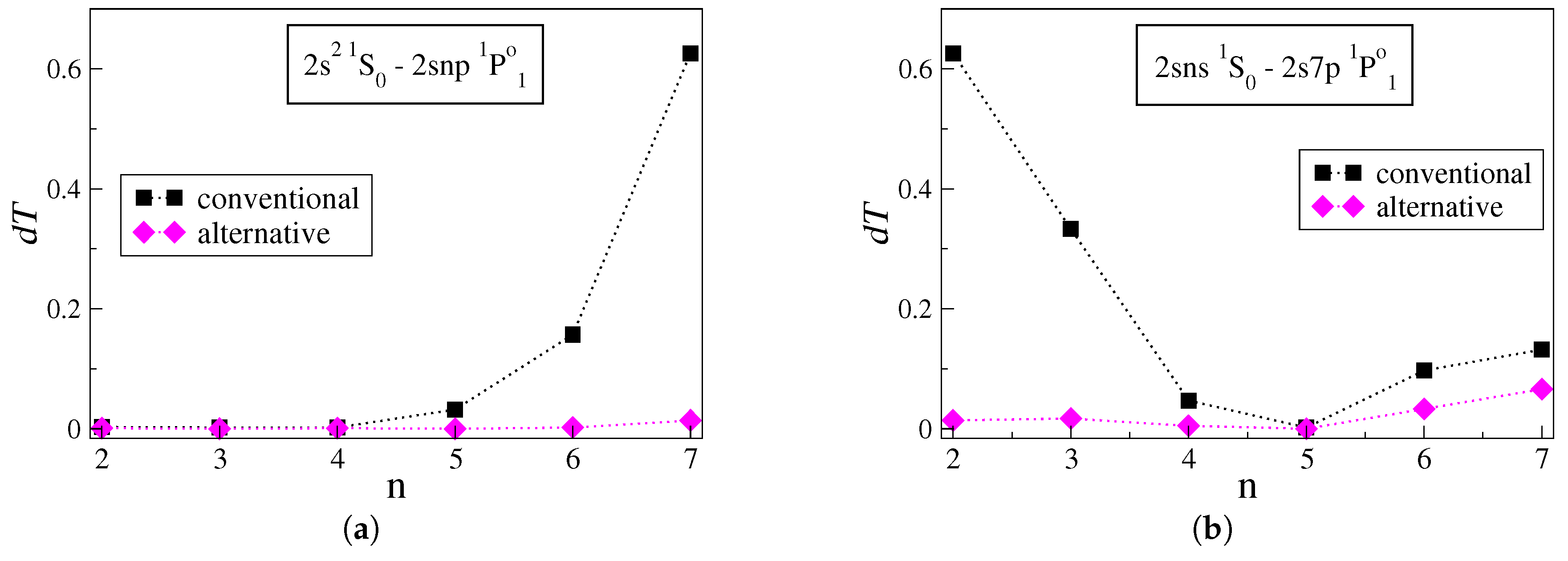
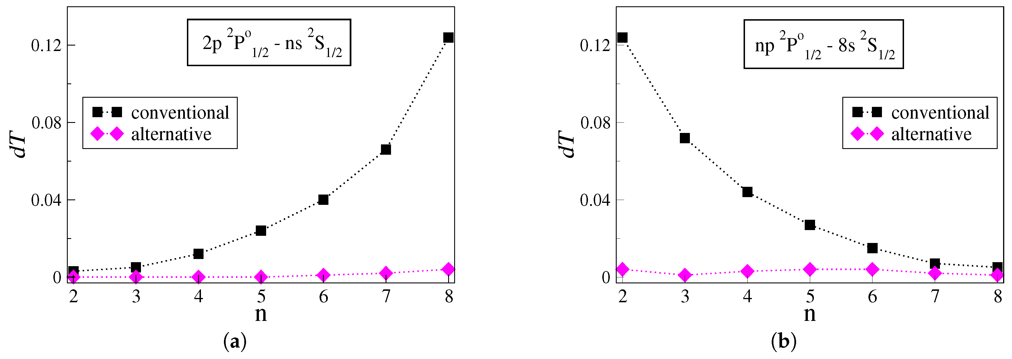
Transition rates A are produced based on the two different computational strategies. In the present computations, the uncertainties in the predicted excitation energies of two states associated with a transition most often cancel out, and consequently, the majority of the evaluated transition energies are ultimately in perfect agreement with the NIST values. The uncertainties of the computed transition rates solely emerge from the disagreement of the computed line strengths in the Babushkin and the Coulomb gauge, which are then reflected in the $dT$ values. When the conventional strategy is applied, most of the transition rates are predicted with uncertainties $dT$ lower than $1\%$ and $5\%$, in lithium-like and beryllium-like carbon, respectively. Yet, for transitions involving high Rydberg states, the uncertainties increase remarkably, especially for the more complex C III ion. The alternative strategy for optimizing the radial orbitals yields transition rates that are overall more accurate. The improvement in accuracy is significant for transitions that involve high Rydberg states.

The uncertainties $dT$ of the transition rates computed with the conventional and alternative approaches are presented and analyzed for groups of transitions in the studied carbon ions. Each group is selected to include transitions between a fixed state and Rydberg states described by electron distributions that are gradually localized farther from the atomic core. Accordingly, Figure 1a,b illustrates the uncertainties $dT$ for the $2p{}^2{P}_{1/2}^{\circ }-ns{}^2{S}_{1/2}$ and $np{}^2{P}_{1/2}^{\circ }-8s{}^2{S}_{1/2}$ groups of transitions in C IV. Similarly, Figure 2a,b illustrates the $dT$ values for the $2s^2{}^1{S}_0-2snp{}^1{P}_1^{\circ }$ and $2sns{}^1{S}_0-2s7p{}^1{P}_1^{\circ }$ groups of transitions in C III.

Figure 1a demonstrates the uncertainties for the series of transitions between the low-lying $2p{}^2{P}_{1/2}^{\circ }$ state and successively higher Rydberg $ns{}^2{S}_{1/2}$ states. The uncertainty $dT$ of the transition rates computed with the conventional approach grows almost exponentially with the increasing principal quantum number n. The transition rate for the $2p{}^2{P}_{1/2}^{\circ }-8s{}^2{S}_{1/2}$ transition, which is the transition between the two states with the largest energy difference in the plot, eventually exhibits the highest uncertainty—$12.4\%$. When the alternative approach is utilized instead, the uncertainties range between $0\%$ and $0.4\%$ for the respective transitions. The same trends are also observed in other groups of transitions in C IV, such as the $2p{}^2{P}^{\circ }-nd{}^{2}D$, the $2s{}^{2}S-np{}^2{P}^{\circ }$, and so forth.

Having as a starting point the $2p{}^2{P}_{1/2}^{\circ }-8s{}^2{S}_{1/2}$ transition, Figure 1b demonstrates the uncertainties for the series of transitions between the high Rydberg $8s{}^2{S}_{1/2}$ state and successively higher Rydberg $np{}^2{P}_{1/2}^{\circ }$ states. As n increases, the transition energy gets smaller. The uncertainties of the transition rates computed with the conventional approach exhibit a nearly exponential decay with increasing n. Similarly to Figure 1a, when following the alternative strategy, the uncertainties in the transition rates are substantially reduced, ranging between $0.1\%$ and $0.4\%$. Other groups of transitions in C IV, such as the $np{}^2{P}^{\circ }-8d{}^{2}D$ series and the $ns{}^{2}S-8p{}^2{P}^{\circ }$ series, follow analogous trends.

Figure 2a displays the $dT$ values for transitions between the low-lying $2s^2{}^1{S}_0$ state and successively higher Rydberg $2snp{}^1{P}_1^{\circ }$ states. Looking at Figure 2a, when the conventional approach is applied the uncertainties $dT$ increase sharply for $n>5$. For the $2s^2{}^1{S}_0-2s7p{}^1{P}_1^{\circ }$ transition, i.e., the transition between the two states with the largest energy difference, the $dT$ rises to $63\%$. The latter is about five times larger than the highest estimated $dT$ value in the figures above. Once more, when the radial orbitals are optimized using the alternative strategy, the uncertainties drop dramatically, ranging between $0\%$ and $1.4\%$ for the respective transitions. More groups of transitions in C III that reveal similar behavior are the $2s2p{}^1{P}_1^{\circ }-2sns{}^1{S}_0$ series and the $2p^2{}^3{P}_0-2snp{}^3{P}_1^{\circ }$ series.

Starting with the $2s^2{}^1{S}_0-2s7p{}^1{P}_1^{\circ }$ transition, Figure 2b displays the $dT$ values for transitions between the high Rydberg $2s7p{}^1{P}_1^{\circ }$ state and successively higher Rydberg $2sns{}^1{S}_0$ states. Likewise, in Figure 1b, the increase in n corresponds to transitions between states that gradually come closer in energy. The uncertainties of the transition rates computed with the conventional approach reduce rapidly as n increases. Applying the alternative strategy results in much lower uncertainties, which extend between $0.5\%$ and $6.6\%$. A similar trend is also observed in the $2snp{}^1{P}_1^{\circ }-2s7s{}^1{S}_0$ series of transitions in C III. Although the last two points in Figure 2b correspond to transitions between states lying close in energy, the uncertainties are comparatively high. Nevertheless, the alternative strategy still predicts the transition rates with lower uncertainties.

Altogether, for transitions between low-lying states, the transition rates are accurately predicted independently of whether the conventional or the alternative computational strategy is employed. Further, when both states involved in a transition in C IV are high Rydberg states, the transition rates are also predicted with high accuracy in both computations. On average, the same holds for transitions between high Rydberg states in C III. The line strengths of transitions between two states close in energy, and with the outer electrons occupying nearly the same region of space, are relatively large, and therefore, weakly affected by the optimization strategy of the radial orbitals. Quite the contrary, transitions between a low-lying state and a high Rydberg state are problematic in both carbon ions. The line strength of transitions between two states with large energy differences, and with the outer electrons occupying different parts of space, take smaller values, which are more sensitive to how the radial orbitals are optimized with regard to correlation.

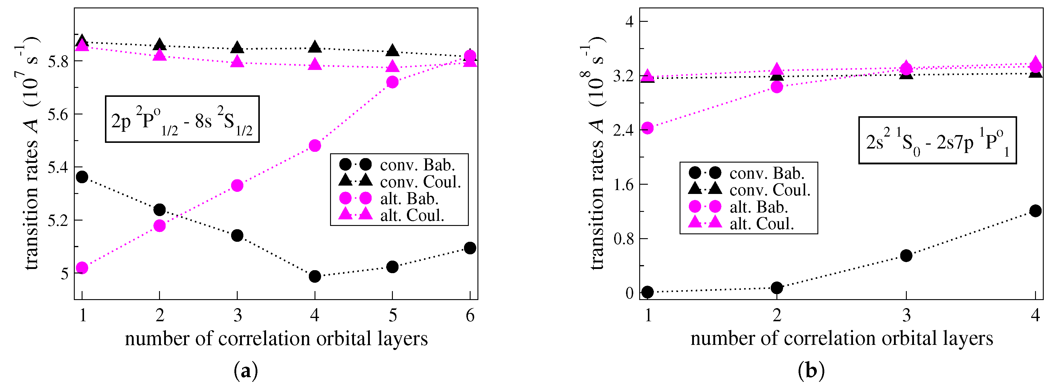
To better understand the origins of the large $dT$ values in transitions between low-lying states and high Rydberg states, the convergences of the individual transition rates $A_B$ and $A_C$, computed in the Babushkin and the Coulomb gauges respectively, are studied with respect to the increasing active set of correlation orbitals. In connection with the figures above, this is done for the $2p{}^2{P}_{1/2}^{\circ }-8s{}^2{S}_{1/2}$ transition in C IV (see Figure 3a) and $2s^2{}^1{S}_0-2s7p{}^1{P}_1^{\circ }$ transition in C III (see Figure 3b); i.e., the transitions with the highest uncertainties $dT$. In Figure 3a,b, the convergences of the $A_B$ and $A_C$ values are illustrated for the two different computational approaches.

As seen in Figure 3a,b, when the computations are performed in the alternative manner, the transition rates given by $A_B$ and $A_C$ ultimately come really close in value. Considering the small final $dT$ value, the agreement between the $A_B$ and $A_C$ values is expected. One observes that the transition rate given by $A_C$ is rather stable with respect to the increasing orbital set. The $A_C$ value varies by only $1\%$ and $6.2\%$ for each of the transitions displayed in the figures below. On the contrary, the $A_B$ value varies by $13.7\%$ and $27.2\%$, respectively. In the $2p{}^2{P}_{1/2}^{\circ }-8s{}^2{S}_{1/2}$ transition, it takes five correlation layers for the $A_B$ value to start converging, while in the $2s^2{}^1{S}_0-2s7p{}^1{P}_1^{\circ }$ transition it takes three layers of correlation orbitals for the $A_B$ value to converge.

Looking at Figure 3a,b, when the conventional approach is applied, the individual $A_B$ and $A_C$ values do not converge, as the large final uncertainties $dT$ reveal. The transition rate given by $A_C$ is, however, again stable and is also consistent with the $A_B$ and $A_C$ values provided by the alternative computational strategy. Throughout the optimization of the radial orbitals in the conventional manner, the $A_C$ value varies by only $0.9\%$ and $2.3\%$ for each of the transitions displayed in Figure 3a,b, respectively. Although it seems that the $A_B$ values will eventually approach the $A_C$ ones, this would require a very large orbital basis, which is beyond the reach of the available computational resources. One may deduce that when the conventional computational strategy is applied the transition rates $A_B$, computed in the Babushkin gauge, are problematic and unreliable.

5. Discussion

Transition data, such as transition rates A, are expressed in terms of reduced matrix elements of the transition operator (see Equation (5)), which can be computed in different gauges. According to Equation (10), the uncertainty of the computed A values is assessed by the agreement of the transition rates computed in the different gauges. Computations of reduced matrix elements in different gauges, however, probe separate parts of the wave functions. Hence, the radial parts of the wave functions must be well approximated as a whole to obtain gauge invariant transition rates.

For transitions between low-lying states, both computational strategies yield reduced matrix elements of the transition operator that almost reach gauge invariance, and the transition rates are, overall, accurately predicted. There are enough correlation orbitals spatially localized between the core and the inner valence orbitals that make up the low-lying states. As a result, the inner parts of the wave functions are adequately approximated. Moreover, the spectroscopic outer valence orbitals, which make up the higher Rydberg states and are localized farther from the atomic core, improve the description of the outer parts of the wave functions for representing the low-lying states, ensuring that they have the correct asymptotic behavior. The radial parts of the latter wave functions are then effectively described at all r values, being insensitive to the choice of the optimization strategy with regard to correlation.

For transitions between a low-lying state and a high Rydberg state, the conventional computational strategy fails to produce accurate transition rates. The correlation orbitals are significantly contracted compared to the outer Rydberg orbitals. Further, there are no spectroscopic orbitals farther localized to correct for the fact that the asymptotic behavior of the tail of the wave functions that represent the higher Rydberg states is not well approximated. Thus, the Babushkin gauge that probes the outer part of the wave functions does not produce trustworthy results. The inner parts of the wave functions representing the higher Rydberg states are, however, adequately approximated, and as a result, the Coulomb gauge yields transition rates that are more reliable (see also, Figure 3a,b).

The alternative computational strategy generates correlation orbitals that are more extended, increasing the overlap with the spectroscopic orbitals that make up the higher Rydberg states. In this case, the correlation orbitals are properly localized to ably describe the asymptotic behavior of the outer part of the wave functions representing the higher Rydberg states. That being so, after the final MCDHF and RCI computations in the alternative manner, the reduced matrix elements of the transition operator are practically gauge invariant and the transition rates are also accurately predicted for the transitions between low-lying states and high Rydberg states (see also, Figure 3a,b).

The radial transition integrals (8) and (9) that take part in the computations of the reduced matrix elements of the transition operator have an upper integration bound that goes to infinity. In (8) and (9), $P(r)$ and $P^{\prime }(r)$ are the radial parts of the spectroscopic and correlation orbitals that are included in the computations. If we express the transition integrals as a function of the upper integration bound R, we get

$${\int }_0^{R}P(r)r{P}^{\prime }(r)dr$$

(11)

and

$${\int }_0^{R}P(r)\frac{d}{dr}{P}^{\prime }(r)dr,$$

(12)

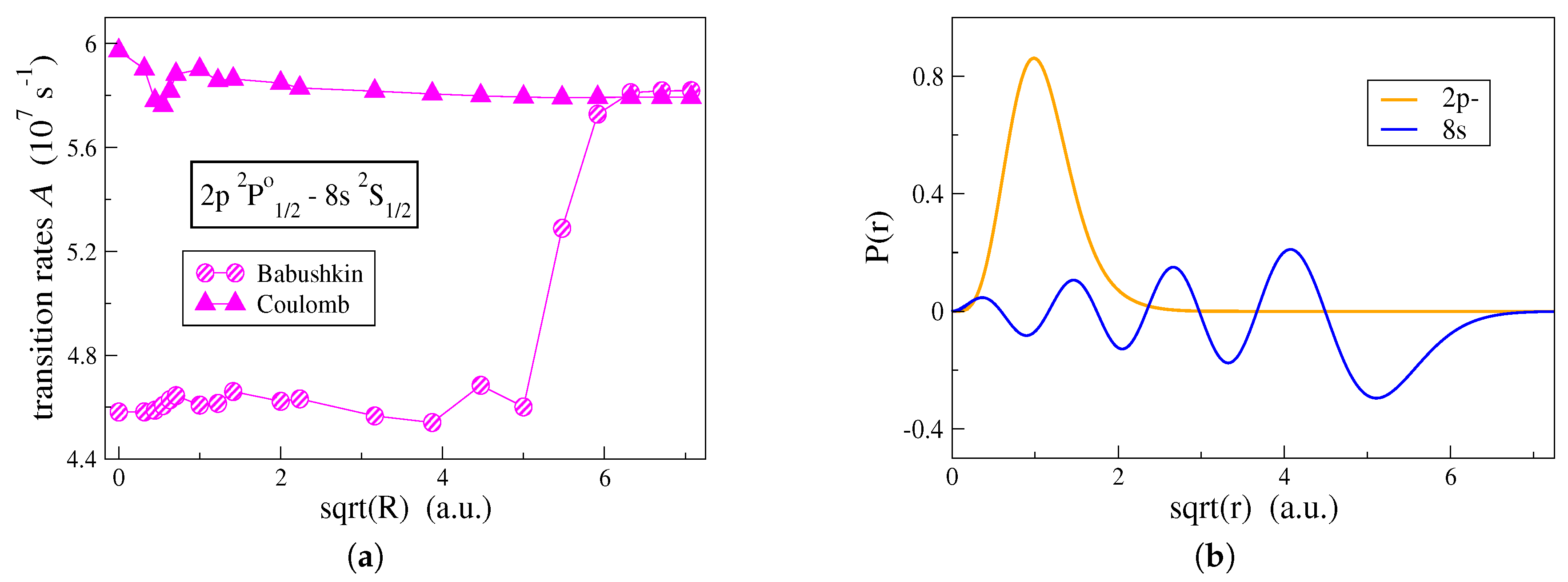
respectively. We can keep $R=\infty$ for the spectroscopic orbitals so that they extend to their full values and only introduce a cut-off value for R in the transition integrals involving correlation orbitals. In this manner, the effect on the transition rate values, from correlation orbitals gradually localized farther from the origin, can be studied. In connection with Figure 3a, the effect that the shape of the correlation orbitals has on the computation of transition rates is, in Figure 4a, examined for the $2p{}^2{P}_{1/2}^{\circ }-8s{}^2{S}_{1/2}$ transition in C IV. In Figure 4a, the transition rates are computed by employing the alternative computational strategy and both Babushkin and Coulomb gauges are displayed. One observes that the two gauges are affected differently by the outer parts of the correlation orbitals.

In Figure 4a, the transition rate computed in the Coulomb gauge is mainly influenced by the correlation orbitals that are localized close to the origin and in the vicinity of the atomic core. Correlation orbitals occupying regions with $\sqrt{R}>1$ have an insignificant effect on the Coulomb gauge. This explains the fact that the conventional computational strategy, which generates more contracted orbitals, still predicts with accuracy, the transition rates in the Coulomb gauge. Oppositely, the Babushkin gauge is hugely affected by the correlation orbitals occupying the region between $\sqrt{R}=5$ and $\sqrt{R}=6$. Looking at Figure 4b, the $8s$ radial orbital, which extends far out from the $1s^2$ atomic core, begins its asymptotic decay at about $\sqrt{R}=5$ and dies out at $\sqrt{R}\approx 6$. Only when we have orbitals extending into this region, the asymptotic behavior of the wave function representing the $8s{}^2{S}_{1/2}$ state is well described, and thus, the Babushkin gauge will yield accurate transition rates. As previously seen, the conventional computational strategy fails to do so.

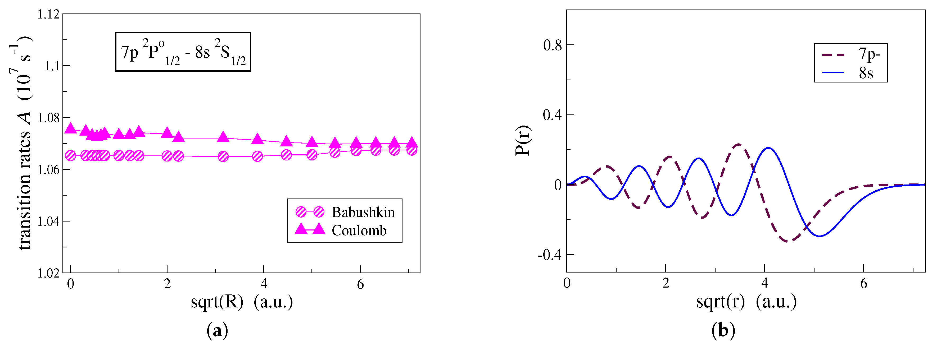
A similar study was performed for a transition between two high Rydberg states. In Figure 5a, the effect of the shape of the correlation orbitals on the computed transition rates is examined for the $7p{}^2{P}_{1/2}^{\circ }-8s{}^2{S}_{1/2}$ transition in C IV. As seen in Figure 5a, correlation has nearly the same effect on both gauges. Although the $7p$ and $8s$ orbitals extend far out from the atomic core (see Figure 5b), correlation orbitals occupying the large R region remain unimportant in the Babushkin gauge. For transitions between states close in energy, the line strengths take large values and the change in the transition rates due to correlation is very small. For this reason, the conventional computational strategy also yields accurate transition rates for transitions between high Rydberg states.

To clarify the fact that the asymptotic behavior of the wave function at large distances is (or is not) well approximated, depending on the alternative (or the conventional) optimization strategy, Brillouin’s theorem [33,34] can be put forward to emphasize the importance of the variational content of the wave functions. When being interested into the description of Rydberg states $1s^{2}nl{}^{2}L$$(L=l)$ in the single-configuration non-relativistic HF approximation, node counting of the valence radial function, $nc=n-l-1$, provides a simple and efficient way to select the desired state in the self-consistent procedure [34]. Each separately optimized state implicitly contains all single-electron excitations $nl\to n^{\prime }l$ of both lower and upper parts of the spectrum, including the continuum $1s^2ϵl$, with the associated interesting property

$$\langle {\Phi }^{\mathrm{HF}}(1s^{2}nl{}^{2}L)|\mathcal{H}|\Phi (1s^2{n}^{\prime }l{}^{2}L)\rangle =\langle {\Phi }^{\mathrm{HF}}(1s^{2}nl{}^{2}L)|\mathcal{H}|\Phi (1s^2ϵl{}^{2}L)\rangle =0,\forall (n^{\prime },ϵ)$$

(13)

where $\mathcal{H}$ is the scalar non-relativistic Hamiltonian that is used in the energy functional to derive the HF equations. The annihilation property of the $(M_L,M_S)$-independent interaction matrix elements between the reference HF CSF built with the optimized HF orbitals, i.e., ${\Phi }^{\mathrm{HF}}$, and all single-electron excitation CSFs $\Phi$, defines Brillouin’s theorem and explains the reasonable accuracy of the HF approximation through the richness of its variational content. The above discussion can be extended to the relativistic framework by considering $n\kappa \to (n^{\prime },ϵ)\kappa$ single-electron excitations and taking for $\mathcal{H}$ the relativistic Hamiltonian that is used for deriving the DHF equations [17].

In the present work, it is hard to define the variational content of the MCDHF approach due to the complexity of the energy functional, but one should keep in mind that the optimization strategy is based (i) on a layer-by-layer approach in which only the last layer is variational while the previous ones are kept frozen, and (ii) on the use of the EOL method targeting, simultaneously, a large number of states for a spectrum calculation. The resulting lack of variational freedom for the individual states can (partially) be counterbalanced by the inclusion of enough interacting states in the Hamiltonian matrix. Going back to the single-configuration approximation case mentioned above, any member of a Rydberg series can be described through configuration interaction involving Brillouin one-electron excitations with a resulting CI-expansion strictly equivalent to the single approximation HF wave function if the basis of single-excitation CSFs is large and rich enough. This equivalence has been exploited to solve convergence problems encountered in the MCHF study of Rydberg series in strontium [35] or to demonstrate the correspondence between different orbital optimization schemes for describing the discrete-continuum interactions in complex systems [36]. In the context of our work, one illustrates the inadequacy of the orbitals obtained in the conventional approach that are used to compensate the lack of variational freedom in the representation of the high-lying Rydberg members. On the contrary, the alternative strategy proposed produces orbitals that have a better localization for describing the single-electron excitations, which would have been implicitly included with a fully optimized MCDHF wave function targeting a single Rydberg state.

6. Summary and Conclusions

The computations of transition data in the systems of lithium-like and beryllium-like carbon are examples of spectrum calculations that involve Rydberg series. In this work, we showed that, independently of the optimization scheme of the radial orbitals, transition parameters corresponding to the lower part of the spectrum are computed with high accuracy. As astronomical spectroscopy raises the demand on atomic data, highly accurate transition parameters are, however, also required for transitions that involve high Rydberg states. We demonstrated how this can be achieved by paying special attention to the optimization scheme of the radial orbitals with respect to correlation. Finally, we showed that the Babushkin gauge should not, by default, be considered as the preferred gauge, and that, in the computations of Rydberg series, it might be required that the transition rates in the Coulomb gauge are used as a reference for the interpretation of astrophysical observations.