Diagnostic of Langmuir Solitons in Plasmas Using Hydrogenic Spectral Lines

Abstract

The development of various spectroscopic diagnostics of relatively weak Langmuir waves in plasmas and their successful implementation have a history of over 50 years. As for spectroscopic diagnostics of Langmuir solitons (i.e., relatively strong Langmuir waves) in plasmas, there have only been very few theoretical papers. The most promising result so far was based on using satellites of the dipole-forbidden spectral lines of He, Li, or He-like and Li-like ions. It was shown that, in the case of Langmuir solitons, the peak intensity of the satellites of the dipole-forbidden lines can be significantly enhanced—by orders of magnitude—compared to the case of non-solitonic Langmuir waves. This distinctive feature of satellites under Langmuir solitons allows them to be distinguished from non-solitonic Langmuir waves. In the present paper, we perform a general study of the effects of Langmuir solitons on arbitrary spectral lines of hydrogen or hydrogen-like ions. Then, using the Ly-beta line as an example, we compare the main features of the profiles for the case of the Langmuir solitons with the case of the non-solitonic Langmuir waves of the same amplitude. We also show how the line profiles depend on the amplitude of the Langmuir solitons and on their separation from each other within the sequence of the solitons.

1. Introduction

The development of various spectroscopic diagnostics of relatively weak Langmuir waves in plasmas and their successful implementation have a history of over 50 years (see, e.g., books [1,2,3] and references therein). As for spectroscopic diagnostics of Langmuir solitons (i.e., relatively strong Langmuir waves) in plasmas, there have only been very few theoretical papers, as follows.

In paper [4], the author calculated analytically the shape of satellites of dipole-forbidden lines in a spectrum spatially integrated through a Langmuir soliton (or through a sequence of Langmuir solitons separated by a distance L). The dipole-forbidden lines are the characteristic feature of He and Li spectral lines (or of the spectral lines of He-like and Li-like ions); Langmuir waves can cause the appearance of satellites of the dipole-forbidden lines. The main result of paper [4] (presented also in Section 7.3 of book [1]) is the following.

In the case of Langmuir solitons, the peak intensity of the satellites of the dipole-forbidden lines can be significantly enhanced—by orders of magnitude—compared to the case of non-solitonic Langmuir waves. This distinctive feature of satellites under Langmuir solitons allows them to be distinguished from non-solitonic Langmuir waves.

As for using hydrogenic spectral lines (in distinction to the above method based on the dipole-forbidden spectral lines of He, Li, and He-like and Li-like ions), Hannachi et al. [5] performed simulations to find the effect of Langmuir solitons on the hydrogen Lyα line. The effect was an additional broadening. However, even at the low electron density Ne = 10¹⁴ cm⁻³, the effect was very small compared to the Stark broadening by plasma microfields. Moreover, the additional broadening rapidly diminished with the increase of Ne, so there would be practically no additional broadening at Ne > 10¹⁵ cm⁻³. In paper [6], Hannachi et al. added a magnetic field into consideration and performed simulations at the electron density Ne = 10¹³ cm⁻³. However, this electron density is unrealistic (too low) for the modern tokamaks (applications to which were hoped by the authors of paper [6]), and again, the additional broadening would rapidly diminish for more realistic (higher) values of Ne. Therefore, it seems that the results by Hannachi et al. [5,6] would not be useful for the experimental diagnostics of Langmuir solitons. 1

Therefore, in the present paper, we perform a general study of the effects of Langmuir solitons on arbitrary spectral lines of hydrogen or hydrogen-like ions. Then, using the Ly-beta line as an example, we compare the main features of the profiles for the case of the Langmuir solitons with the case of the non-solitonic Langmuir waves of the same amplitude. We also show how the line profiles depend on the amplitude of the Langmuir solitons and on their separation from each other within the sequence of the solitons.

2. Brief Overview of the Theory

Langmuir solitons (or a sequence of Langmuir solitons separated by a distance L) have the following form in space [9]:

F(x, t) = E(x) cos ωt, E(x) = E₀/ch(x/λ), λ << L

(1)

Here,

$$\mathsf{\omega }={\mathsf{\omega }}_{\mathrm{pe}}-3T_{e }/\left(2{\mathrm{m}}_{\mathrm{e}}{\mathsf{\omega }}_{\mathrm{pe}}{\mathsf{\lambda }}^2\right),$$

(2)

where ω_pe is the plasma electron frequency, and λ is the characteristic size of the soliton. For diagnosing solitons, it is necessary not only to find experimentally an electric field oscillating at the frequency ~ω_pe but also to make sure that the spatial distribution of the amplitude corresponds to the formfactor E(x) from Equation (1).

We start by considering the splitting of hydrogenic spectral lines at the fixed value of x. Then, we will average the result over the formfactor E(x) from Equation (1) to produce new results.

In 1933, Blochinzew considered the splitting of a model hydrogen line, consisting of just one Stark component, under a linearly polarized electric field E₀ cos ωt and showed that it splits in satellites separated by pω (p = ± 1, ± 2, ± 3, …) from the unperturbed frequency ω₀ of the spectral line [10]:

$$\mathrm{S}\left(\Delta \mathsf{\omega }/\mathsf{\omega }\right)={\displaystyle \sum }_{\mathrm{p}=-\infty }^{+\infty }[{{\mathrm{J}}_{\mathrm{p}}}^2\left({\mathrm{X}}_{\mathrm{k}}\mathsf{\epsilon }\right)]\left(\mathsf{\delta }\left(\frac{\Delta \mathsf{\omega }}{\mathsf{\omega }}\right)-\mathrm{p}\right),$$

(3)

where J_p(u) are the Bessel functions, and ε is the scaled amplitude of the field:

ε = 3ħE₀/(2Z_rm_eeω),

(4)

Here, Z_r is the nuclear charge of the radiating atom/ion and

$${\mathrm{X}}_{\mathrm{k}}=\mathrm{nq}-{\mathrm{n}}_0{\mathrm{q}}_0,$$

(5)

where n, q and n₀, q₀ are the principal and electric quantum numbers of the upper and lower energy levels, respectively, involved in the radiative transition. Physically, the larger the product X_kε, the greater is the phase modulation of the atomic oscillator.

In paper [11], Blochinzew’s result was generalized to profiles of real, multicomponent hydrogenic spectral lines in the “reduced frequency” scale as follows (also presented later in book [3], Section 3.1)

$$\mathrm{S}\left(\Delta \mathsf{\omega }/\mathsf{\omega }\right)={\displaystyle \sum }_{\mathrm{p}=-\infty }^{+\infty }\mathrm{I}\left(\mathrm{p},\mathsf{\epsilon }\right)\mathsf{\delta }\left(\Delta \mathsf{\omega }/\mathsf{\omega }\right)-\mathrm{p}),$$

(6)

where

$$\mathrm{I}\left(\mathrm{p},\mathsf{\epsilon }\right)=[{\mathrm{f}}_0{\mathsf{\delta }}_{\mathrm{p}0}+2{\displaystyle \sum }_{\mathrm{k}=1}^{\mathrm{kmax}}{\mathrm{f}}_{\mathrm{k}}{{\mathrm{J}}_{\mathrm{p}}}^2\left({\mathrm{X}}_{\mathrm{k}}\mathsf{\epsilon }\right)]/({\mathrm{f}}_0+2{{\displaystyle \sum }}^{\text{}}{\mathrm{f}}_{\mathrm{k}}),$$

(7)

Here, f₀ is the total intensity of all central Stark components, and f_k is the intensity of the lateral Stark component with the number k = 1, 2, …, kmax.

In the practically important case of the strong modulation (X_kε >> 1) from Equations (3), (6), and (7), it follows that there could be numerous satellites of significant intensities. Frequently, the individual satellites merge together by broadening mechanisms, so only the envelope of these satellites can be observed. The most intense part of the satellite envelope has the shape of the Airy function, as shown in paper [11] and reproduced in book [3], Section 3.1. Based on these analytical results, the following practical formula has been derived and presented in [3,11] (Section 3.1) for the position p_max of the satellite having the maximum intensity (and thus corresponding to the experimental peak):

p_max(a) = a + (a/2)^1/3d_Ai = a − 0.809(a)^1/3, a = X_kε

(8)

where d_Ai = −1.019 is the first zero of the derivative of the Airy function.

3. New Results

The averaging over the formfactor E(x) from Equation (1) starts by substituting E(x) into the argument of the Bessel function in Equation (3) and integrating over x from −λ to λ, or equivalently:

$$\mathrm{f}\left(\mathrm{p},\mathrm{a},\mathrm{b}\right)=\left(1/\mathrm{b}\right)\underset{-\mathrm{b}/2}{\overset{\mathrm{b}/2}{{\displaystyle \int }}}\mathrm{dy}{{\mathrm{J}}_{\mathrm{p}}}^2\left[\mathrm{a}/\mathrm{ch}\left(\mathrm{y}\right)\right],$$

(9)

where we denote

b = L/λ, y = x/λ.

(10)

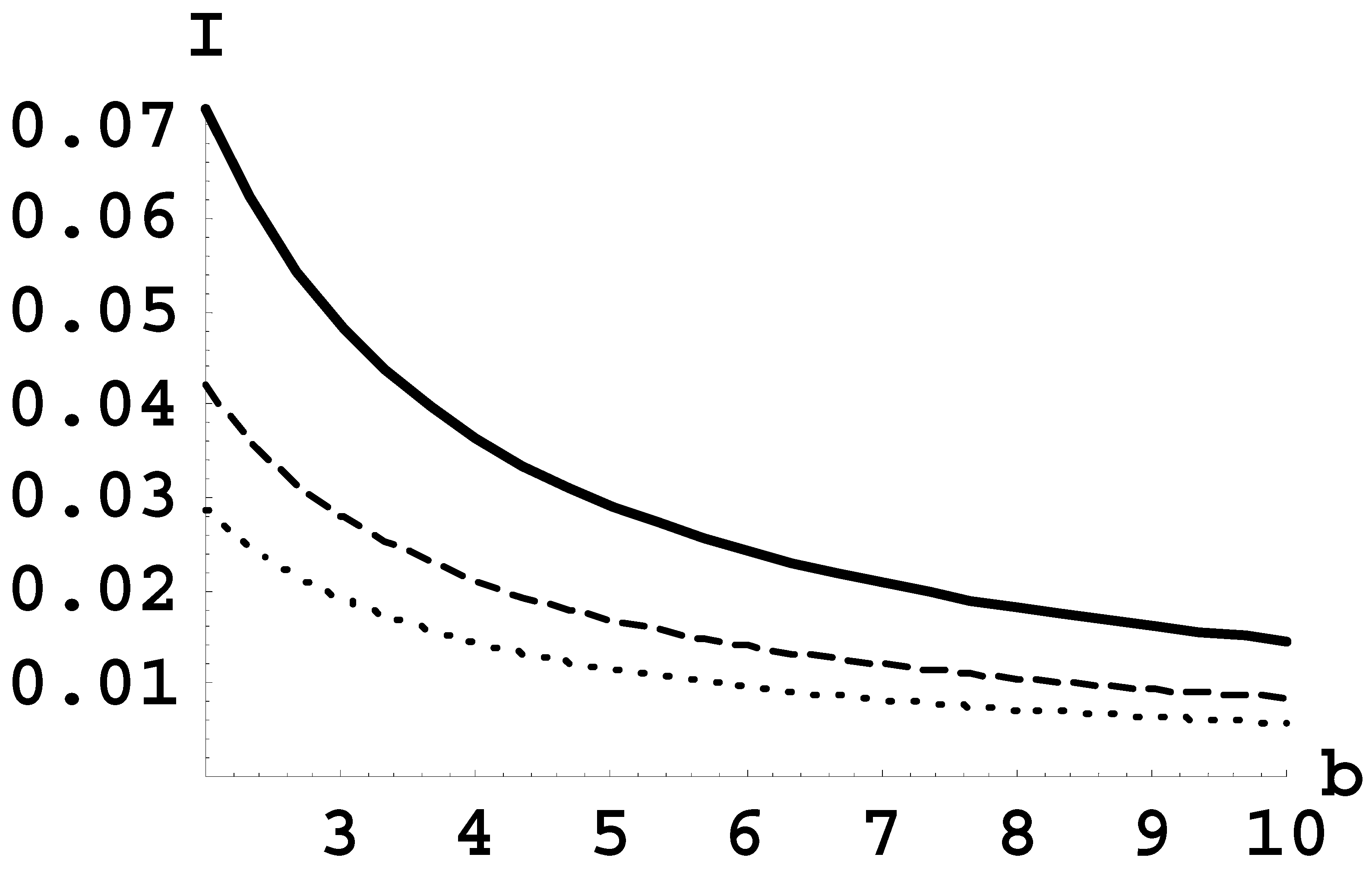
Because the maximum intensity has the satellite at the position p_max(a), given by Equation (8), its spatially integrated intensity from Equation (9) is I = f[p_max(a), a, b]. Figure 1 shows I versus b for a = 10 (solid line), a = 15 (dashed line), and a = 20 (dotted line). It can be seen that the integrated intensity of the most prominent satellite decreases as either a increases (e.g., the field amplitude E₀ increases) or as b increases (i.e., the distance L between Langmuir solitons in the sequence increases).

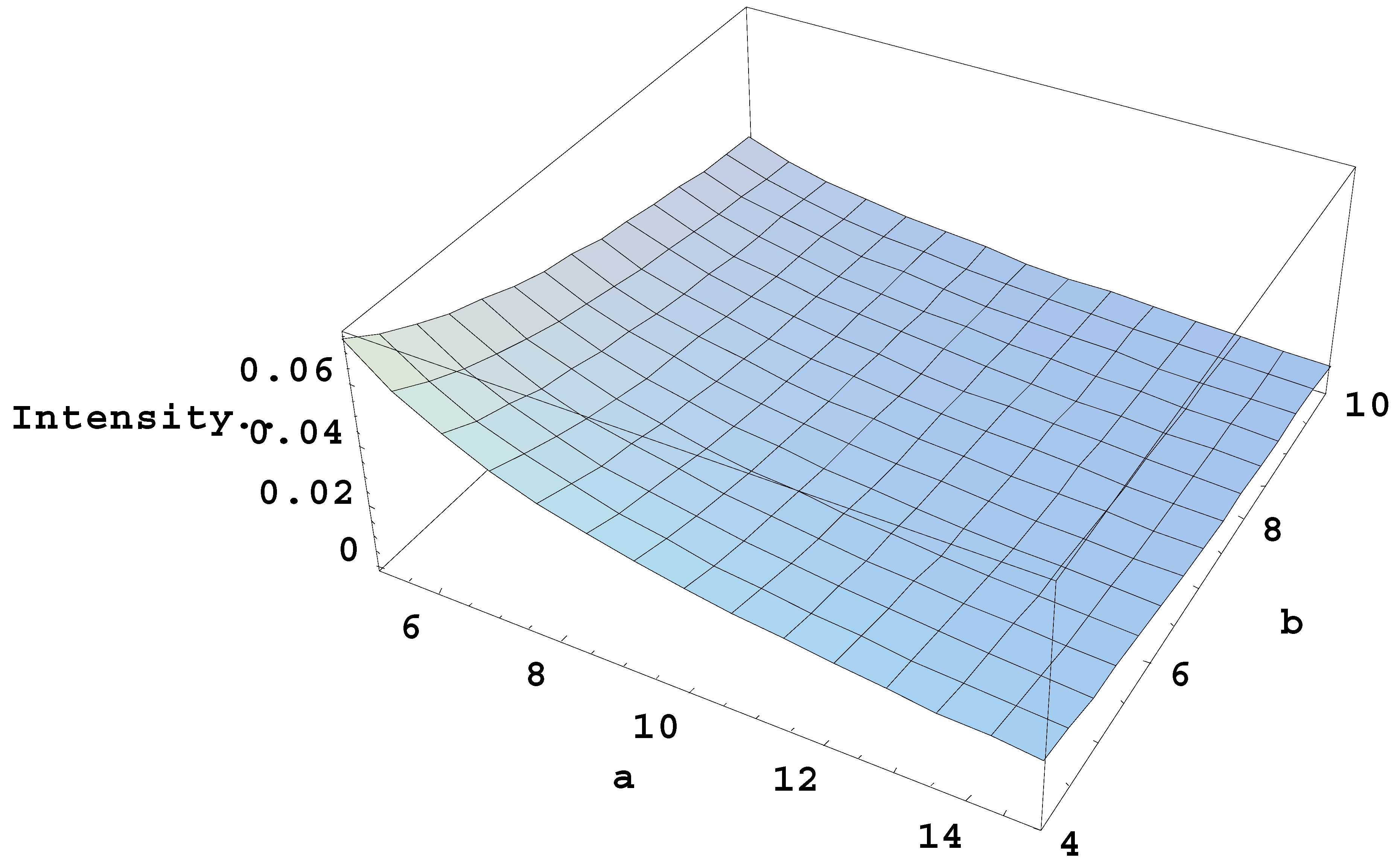
Figure 2 presents a three-dimensional plot of the spatially integrated intensity of the most prominent satellite versus both a and b.

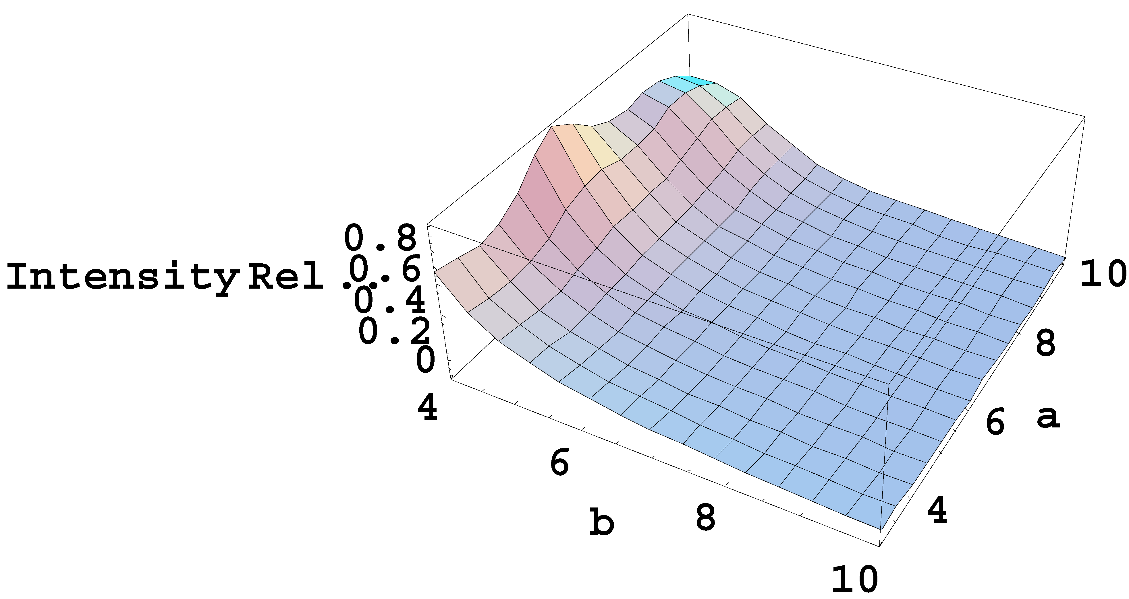
Figure 3 shows a three-dimensional plot of the ratio f[p_max(a), a, b]/ f[0, a, b] versus a and b. This is the ratio of the spatially integrated intensity of the most prominent satellite to the spatially integrated intensity of the “zeroth” satellite, the latter being the intensity at the unperturbed position of the one-component spectral line. It can be seen that this ratio is generally a non-monotonic function of the scaled amplitude a of the solitons electric field.

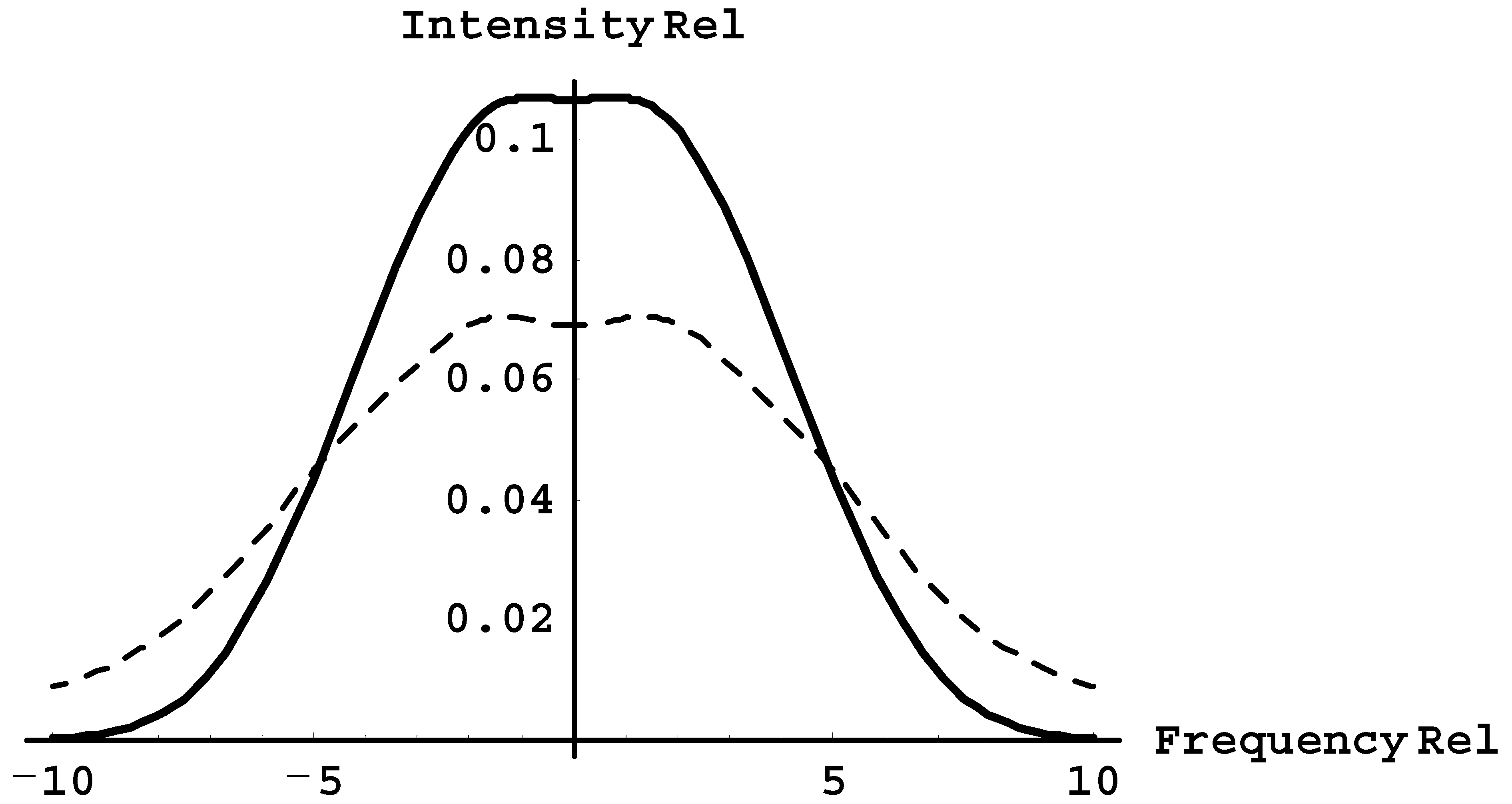
Now, we proceed to real, multicomponent hydrogenic spectral lines. As an example, we use the Ly-beta line in the observation perpendicular to the solitons electric field.

Figure 4 presents the profile of the Ly-beta line versus the scaled distance Δω/ω from the unperturbed position of this line for the (differently) scaled amplitude ε = 3ħE₀/(2Z_rm_eeω) = 1 and the scaled distance b = L/λ = 2 between the Langmuir solitons in the sequence (solid line). Also shown is the corresponding profile for the case of the non-solitonic Langmuir waves for the same value of ε = 1 (dashed line). The direction of the observation is perpendicular to vector E₀. The profiles are continuous (rather than being a set of satellites isolated from each other) because additional broadening mechanisms (the Stark broadening by plasma microfields and the Dopler broadening) were taken into account in amount of δω = 2ω. An example of the fulfillment of the latter relation could be plasmas of multicharged ions produced by a powerful Nd-glass laser, where, at the surface of the critical density, the electron density is N_e = 10²¹ cm⁻³ (or slightly higher due to relativistic effects), and the temperature would be up to T ~ 10³ eV.

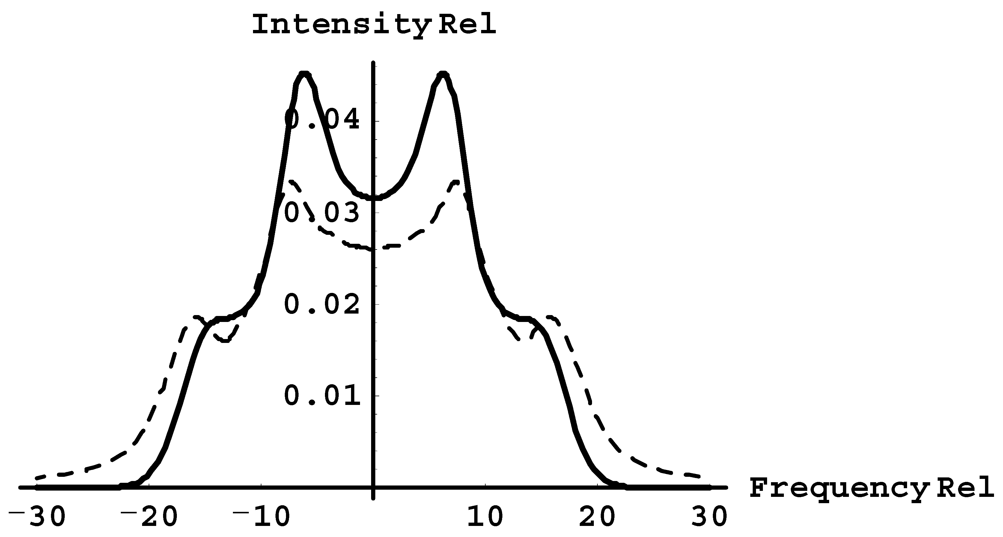
It can be seen that, in the case of the solitons, the profile is narrower than in the non-solitonic case. It can also be seen that both profiles have practically the bell shape without any significant features.

Figure 5 shows the same as Figure 4 but for stronger Langmuir waves, corresponding to ε = 3. Both profiles have features. In the non-solitonic case (dashed line), the profile has two maxima, both in the red and blue sides; in the case of solitons, the primary maximum in each side remains, but the secondary maximum in each side transforms into a shoulder.

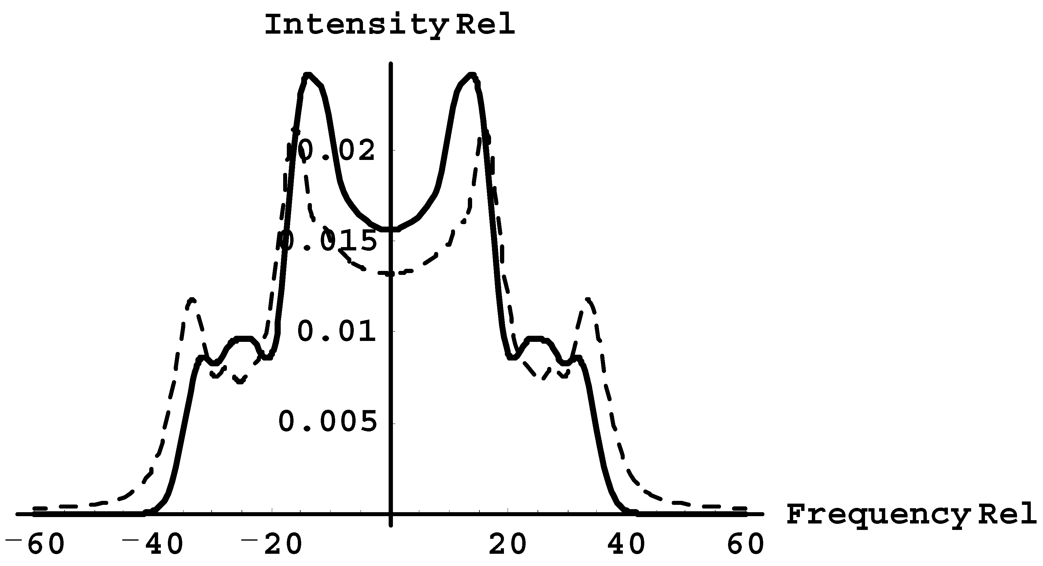
Figure 6 shows the same as Figure 5 but for even stronger Langmuir waves, corresponding to ε = 6. Both profiles have more features than in Figure 5: three maxima both in the red and blue sides. In the case of solitons, the second maximum in each side is more pronounced than for the non-solitonic case. For the third maximum, the situation is opposite; in the case of solitons, the third maximum is less pronounced than for the non-solitonic case.

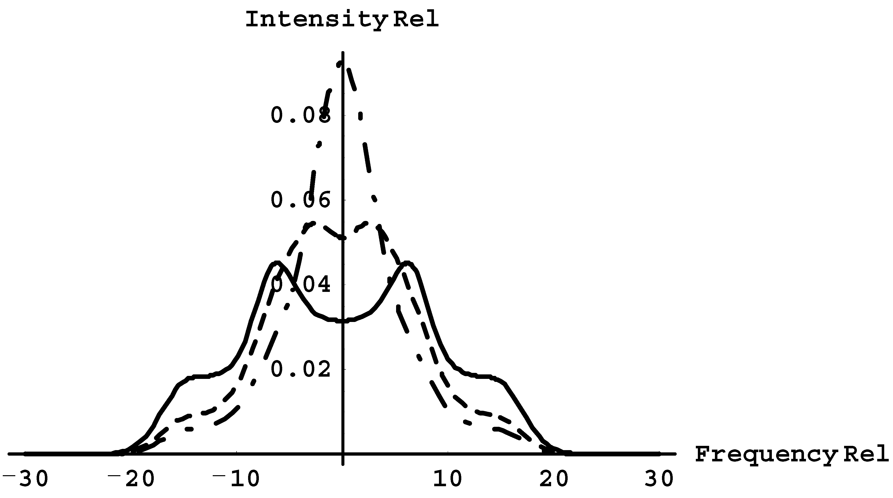
Now, we demonstrate how the Ly-beta profiles for the case of the Langmuir solitons depend on the scaled distance b = L/λ between Langmuir solitons in the sequence. In Figure 7, the Ly-beta profiles corresponding to ε = 3 are presented for b = 2 (solid line), b = 4 (dashed line), and b = 6 (dash-dotted line). It can be seen that, as the scaled distance b = L/λ between Langmuir solitons in the sequence increases, the features (such as maxima, minima, shoulders) gradually disappear.

Therefore, the diagnostic of Langmuir solitons while employing, for example, the Ly-beta line, can be based on the following observation. In the non-solitonic case, there could be distinct secondary maxima in each wing of the line, whereas in the case of solitons, the would-be secondary maxima look more or less like shoulders (see Figure 5 and Figure 6, and the solid line in Figure 7).

4. Conclusions

We studied the general effects of Langmuir solitons on arbitrary spectral lines of hydrogen or hydrogen-like ions. We showed that the integrated intensity of the most prominent satellite in the spectrum of a line component decreases as either the Langmuir field amplitude increases or as the separation between Langmuir solitons in the sequence increases.

For real, multicomponent hydrogenic lines, we used the Ly-beta line as an example to compare the main features of the profiles for the case of the Langmuir solitons with the case of the non-solitonic Langmuir waves of the same amplitude. The outcome was that, for the case of the Langmuir solitons, some maxima in the line profile became less pronounced or even transformed into shoulders.

Finally, we demonstrated that, as the amplitude of the Langmuir solitons increases, more features (such as maxima and minima) appear in the line profiles. We also showed that as the separation between the solitons within their sequence increases, there are less features in the line profiles.

The above results can be used for detecting the Langmuir solitons. They can also be used for determining the amplitude of the Langmuir solitons and their separation from each other in the sequence of solitons.