1. Introduction
Most of our knowledge about atoms derives from spectroscopic studies. Conventional spectroscopy provides precise information about the energy of electronic states in an atom. These states can be represented as poles in the frequency response of the atom to an applied field. A complementary approach can be found in the recently developed technique of tune-out spectroscopy, in which zeros of the atomic frequency response are measured [
1,
2]. Although tune-out measurements are generally more complicated to implement than conventional spectroscopy, it is still possible to achieve high accuracy results [
3,
4,
5,
6,
7].
An important feature of tune-out spectroscopy is that it provides information about the relationship between the atomic response of different states. For example, in between a nearby pair of dipole-allowed transitions there is a zero in the dynamic electric polarizability, where the positive polarizability from one state perfectly cancels the negative polarizability from the other state. The location of the zero depends primarily on the ratio of the electric dipole matrix elements of the two states. While there are techniques to directly measure matrix elements for some states, the ratio determined via tune-out spectroscopy can be much more accurate than the ratio of direct measurements. For instance, our recent tune-out frequency measurement for the rubidium
states improved the accuracy of the matrix element ratio by a factor of 100 compared to direct measurements [
6]. Furthermore, for many states it is difficult to measure the matrix elements directly with good precision. Tune-out spectroscopy can be used in such cases to relate the desired matrix element to that of a more easily measured transition. For instance, Herold
et al. improved knowledge of the
matrix elements in rubidium by a factor of ten by relating them to the better-known
elements [
4].
While these results demonstrate the utility of tune-out spectroscopy, a challenge is that to some degree the frequency of any single response zero depends on all of the accessible states and matrix elements in the atom [
2]. To deal with this, theoretical estimates are used for contributions that are not of direct interest. This introduces additional sources of uncertainty and limits the applicability of the measurements to systems where high-quality theoretical estimates are available.
We present here a technique to reduce this dependence on theory. Up to now, most studies have centered on the scalar response of the atom, which can be obtained by averaging over the atomic spin states and/or the optical polarization of the light. However, spin-polarized atoms also have a strong vector response, which can be measured by varying the light polarization and the spin orientation. The effect on the tune-out wavelength was measured in a recent study by Schmidt
et al. [
7].
Like the scalar response, the vector response depends on multiple transition matrix elements. However, these elements combine in a different way for the scalar and vector quantities. We show here that by making joint measurements of both responses, different contributions to the electric polarizability can be experimentally resolved. This can lead to improved accuracy and can provide experimental information about matrix elements that cannot easily be observed directly.
Of particular significance, it is possible to independently determine the effects of the atomic core and of the infinite manifold of high-lying valence states. The electric polarizability of the ionic core can in some cases be determined directly by Rydberg atom experiments [
8], but such a measurement requires a theoretical correction to account for core-valence interactions in the ground-state atom [
9]. The “tail” contribution from the valence manifold is even more challenging, and no direct measurement of its effect seems possible due to the many states involved [
10].
These core and tail contributions are small but have significant importance. In particular, the well known experimental measurements of parity violation in cesium [
11] can be related to fundamental quantities in high-energy physics, but this requires precise knowledge of atomic dipole matrix elements including the core and tail contributions. Theoretical uncertainty in the tail is currently the dominant source of error in interpreting the experimental results [
10]. Experimental measurement of the tail contribution using the tune-out spectroscopy technique discussed here could therefore be of great utility.
Accurate knowledge of atomic matrix elements is useful for other applications as well. Important examples include the prediction and characterization of Feshbach resonances in atomic collisions [
12,
13] and estimation of blackbody shifts for atomic clocks [
14,
15].
This paper presents calculations regarding the utility of vector tune-out measurements in alkali atoms, with rubidium as a specific example.
Section 2 presents an analysis of the lowest tune-out frequency, while
Section 3 shows that more information can be obtained by combining measurements at several tune-out frequencies.
Section 4 discusses experimental considerations, and
Section 5 offers conclusions.
2. Vector Tune-out Analysis
The response of an atom to an off-resonant optical field at frequency
ω is largely governed by the electric polarizability,
. For an alkali atom in state
i, this can be expressed as [
16]
The sum is over all excited states
f of the valence electron, and
is the transition frequency between
i and
f. Here we neglect hyperfine structure and let
i and
f represent individual Zeeman states
and
. The matrix element
is
where
is the dipole operator and
is the polarization vector of the light. Given the
S ground state for alkali atoms, only excited
P states will appear in the sum. The polarizability contribution of the core electrons is represented by
, while
is the correction accounting for core-valence interactions [
2].
Using Equation (
1), the interaction energy of the atom with the field can be expressed as
where
is the electric field of the light and the angle brackets denote a time average.
It is often convenient to decompose Equation (
1) into spherical tensor components. The interaction energy can then be expressed as [
17]
where the
is the scalar component and
is the vector component. The quantization axis for the states is defined by a magnetic field pointing in the
direction. The polarizability components themselves can be calculated in terms of reduced matrix elements
as
and
Here the sums over excited states
f include
and
but not
. The reduced matrix elements
are defined using the convention of, for instance, Reference [
2]. In
,
is either −2 or +1 depending on the excited state angular momentum. Since the ionic core has zero spin, the core term
has only a scalar contribution. The core-valence term
can have a vector component as well, denoted by
.
High precision measurements require that hyperfine structure be taken into account, resulting in more complicated formulas for the
components [
17]. However, this will not produce any qualitative changes to the results described here.
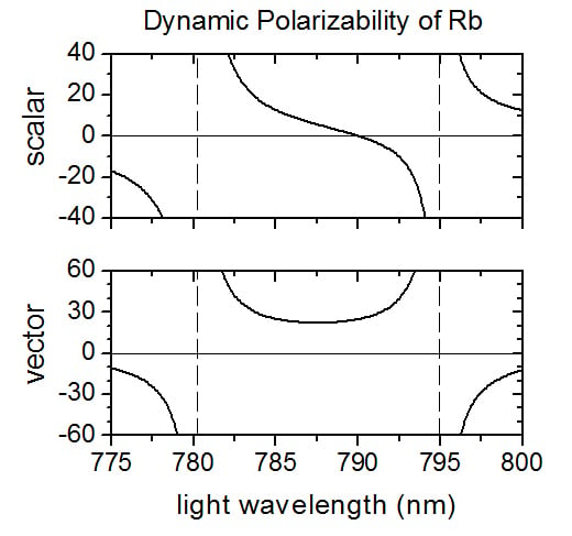
Tune-out spectroscopy locates frequencies where . Our concern here is to relate the value of to the dipole matrix elements and core contributions. We consider first the lowest tune-out frequency for Rb atoms, located in between the transition at 795 nm and the transition at 780 nm. The atoms are initially spin polarized with .
Figure 1 shows the scalar and vector polarizabilities in this wavelength range. The atomic parameters used for the calculation are summarized in
Table 1 and
Table 2, and will be discussed further below. The tune-out frequency
is the solution of
, where
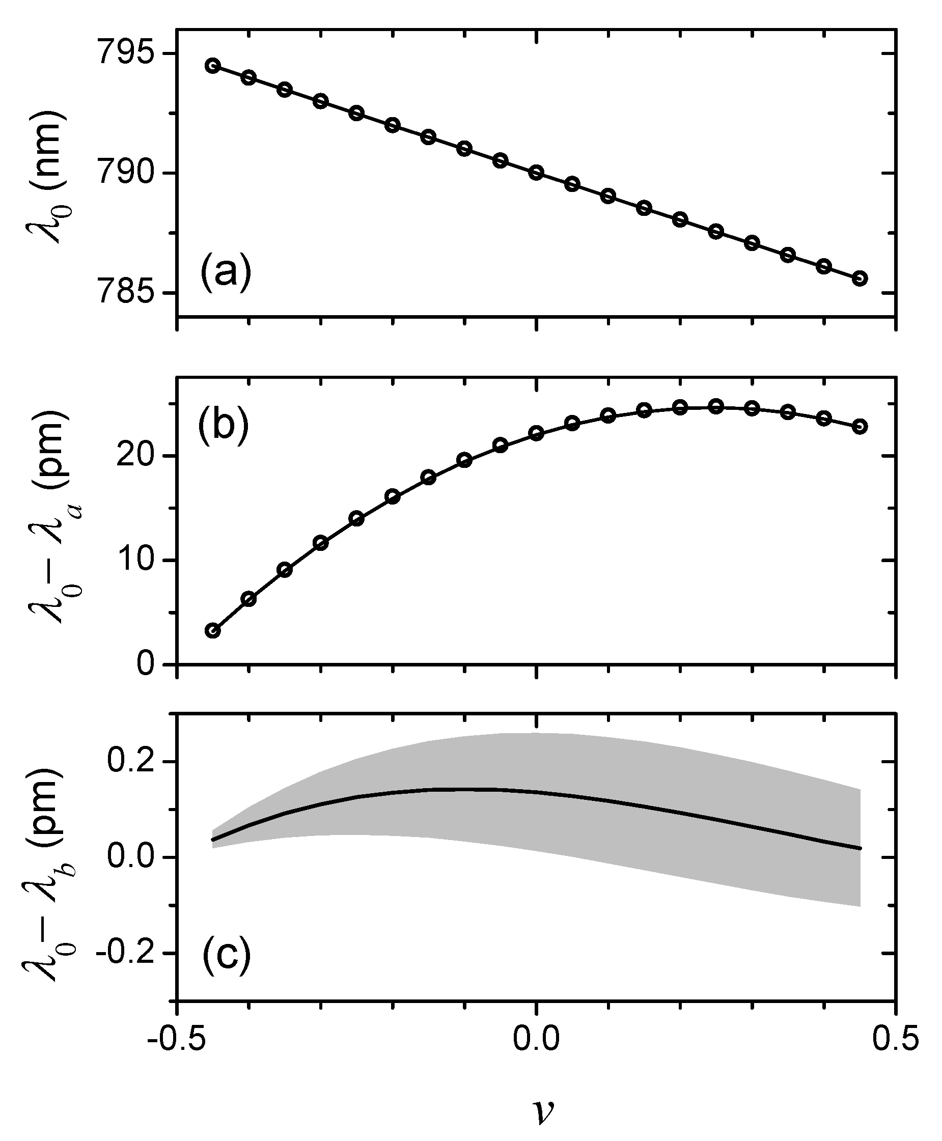
can vary from −1/2 to +1/2 as the light polarization and magnetic field direction are adjusted. The data points in
Figure 2a plot the wavelengths
corresponding to numerical solutions for
at different
v. The dominant behavior is clearly linear, which can be understood as follows:
In this frequency range, the two
transitions dominate the sums in Equations (
4) and (
5). In the limit that the fine structure splitting is small compared to
ω, it is reasonable to keep only the
terms and approximate them as
where we abbreviate here
for
,
for
, and
for
. We can also approximate
, as the state degeneracies would suggest. The root of Equation (
6) is then easily found as
for
. The corresponding wavelength is plotted as the line in
Figure 2a, and evidently accounts for the main features of the exact solution. At this level, no useful information is obtained from the tune-out measurement, since the fine structure splitting is already known from conventional spectroscopy.
However, the deviations between the linear approximation and the exact solution are significant, as seen in
Figure 2b. These deviations can be compared to the 0.03-pm accuracy of the experimental measurements in [
6]. To analyze these deviations we develop a more accurate approximation. We retain the
states as the dominant terms, and in particular assume that the frequency variation of the other terms in Equations (
4) and (
5) can be neglected since those states are far from resonance. We also allow for a non-ideal matrix element ratio as
. The polarizability can then be expressed as
for
and
We use
au as a common normalizing factor [
6,
18]. The sums in
A and
B are over valence states with
. We evaluate these terms at
. Since the
term includes a small denominator, we approximate it more accurately using
from Equation (
7). This gives
independent of
v to lowest order.
The solution of
can be obtained analytically as
, and then the effect of the small terms give an approximate root
with the derivative evaluated at
. Expanding this to second order in the fine-structure splitting Δ and to first order in the small parameters
A,
B and
yields a cubic polynomial in
v,
with
and
This approximate solution is shown as the curve in
Figure 2b, and agrees well with the full numerical results. The difference between the polynomial approximation and the full solution is shown in
Figure 3c, where the shaded area represents the uncertainty in the theoretical parameters of the model.
It is observed that the polynomial approximation
depends on the non-
state parameters only through the combinations
and
B. The first combination can be obtained anyway from a scalar measurement with
, so
B is of more interest here. The sum in Equation (
11) can be broken into a finite number of terms from
to some
, plus an infinite sum over states very near the dissociation limit. It is possible to obtain accurate theoretical estimates for the matrix elements in the finite terms. For instance,
Table 1 shows results up to
taken from Reference [
6], which together provide a contribution to
B of
au.
For the remaining tail contribution, theoretical estimates are uncertain due to significant dependence on the calculational methods used. The estimates used in Reference [
6] were
with
au and
au, both with error estimates comparable to their values. In Equation (
19),
corresponds to the ionization frequency at a wavelength of 297.8 nm. The contribution of these terms to
B will be
au.
We are not aware of any previous calculations of the vector core contribution
. The scalar term
is calculated to be
au [
19]. From the general form of the polarizability expansion, we expect the vector term to be smaller by a factor on the order of
where
is the lowest excitation frequency of the ionic core. For Rb
this lies at a wavelength of 74 nm, so we expect
au. If we estimate the uncertainty as comparable to this value, we obtain a total estimate for
B of
au, with uncertainty dominated by the tail and core terms. A precise measurement of
B would therefore provide an experimental constraint on these uncertain quantities.
To estimate the feasible measurement accuracy, we use the error estimates discussed in Reference [
6]. The reported wavelength error
pm corresponds to
au. Considering, for instance, the linear term
from Equation (
16) and assuming that
v can be varied by about one, we get an expected accuracy
Since this is smaller than the theoretical uncertainty, it can be expected that experimental measurements will provide useful information.
3. Multiple Tune-out Frequency Analysis
The previous discussion illustrates that measurement of vector tune-out wavelengths can provide an experimental constraint on parameters of theoretical interest, thanks to the differing character of their polarization dependence. However, the measurements near 790 nm cannot provide definitive values for these parameters. We show now that by combining vector measurements around multiple tune-out frequencies, we can obtain more direct results. This is possible because the different components have different frequency dependence, in addition to the polarization dependence. By varying both the frequency and polarization, enough information can be obtained to extract the values of individual contributions.
After the tune-out wavelength at 790 nm, the next longest tune-out wavelengths in Rb are a pair associated with the states near 420 nm. The scalar zeros were measured by Herold et al. to be 423.018(7) nm and 421.075(2) nm. We show that vector measurements near these wavelengths are sufficient to extract the polarizability terms of interest. Another pair of tune-out wavelengths near 360 nm is associated with the 7P states, and is also reasonably accessible.
The polarizabilities near 420 nm can be calculated using the same Equations (
4) and (
5). To good approximation, the core terms should be the same as at 790 nm, since
is still much larger than
ω [
16].
Figure 3 shows plots of the tune-out wavelengths as functions of
v. The behavior is more complicated here since there are comparable contributions from several states, and an algebraic analysis involves solutions to high-order polynomials. So, rather than developing an analytical model, we consider a numerical fit to artificially generated synthetic data.
To generate a synthetic data set, we calculated
for nine
v values near each of the three tune-out wavelength at 790 nm, 423 nm, and 421 nm. To each point we added a random experimental error. To account for variations in experimental sensitivity, we used an error estimate
with
and
calculated numerically at each measurement point. Here
accounts for the overall experimental sensitivity and
accounts for experimental polarization control. From the
results in [
6] we estimate
au and
. The resulting
values are used as the standard deviation for a random Gaussian error. This generated a total of 27 simulated data points
.
To this data set we fit the solutions of
, using seven adjustable parameters. Three are the matrix element ratios
,
and
where
. Two more parameters are the core polarizabilities
and
. The last two parameters describe the tail contributions. We define effective matrix elements
so that the scalar tail contribution is
We normalize these and use fit parameters
. For excited states
to 12, we use the theoretical matrix elements in
Table 1.
Values for the fit parameters were obtained by minimizing
. We generated 100 different synthetic data sets using the same model parameters but different errors. We fit each, and the average value of the fitted parameters agreed well with the model parameters used. We report the standard deviation of the fitted parameters as an estimated error for the procedure. The results are shown in
Table 2. The core and tail parameters have been multiplied by
to report the physically interesting values. It can be observed that the fitting errors are generally lower than current accuracies, and in particular that definite values for the core and tail contributions can be obtained.
To gain a clearer understanding of why measuring multiple tune-out wavelengths is effective, we can return to the decomposition of the polarizability used in
Section 2. There, measurements provided a value for the
B parameter and for a combination of
R and
A. The more complicated dependence on
v observed at the 421 nm and 423 nm zeros breaks the degeneracy between
A and
R, so that at each of these zero a value for
A,
B, and
R can be determined. The unknown contributions to
A and
B are the core and tail terms, which have distinctly different frequency dependence. By relating the measurements near 790 nm and 420 nm, these components can be distinguished and the core parameters isolated. Since
A and
B depend differently on the
and
tail parameters, these components can be distinguished as well.
4. Experimental Implementation
We briefly discuss how an experimental measurement of the type described might be implemented. A variety of experimental techniques have been demonstrated for tune-out spectroscopy, including atom interferometry [
3,
6], Bragg coupling in an optical lattice [
4,
7,
20], or direct dipole force measurements [
5]. The highest precision has been achieved with the method of [
6]. Here an atom interferometer is implemented in a time-orbiting magnetic trap potential. An off-resonant standing-wave laser is used to split and recombine the atoms in a Bose-Einstein condensate. While the atomic wave packets are separated, one packet is exposed to a focused traveling-wave Stark laser beam. This shifts the energy of the atoms according to Equation (
2), which can then be detected as a phase shift in the interferometer output. The tune-out wavelength is located by adjusting the Stark laser frequency such that no phase shift is observed.
This method is intrinsically very sensitive. For the measurements proposed here, however, it is also necessary to precisely control the polarization of the Stark beam. This is difficult to achieve with purely optical techniques because the vacuum window through which the beam passes can change the polarization in an uncontrolled way due to stress-induced birefringence. In the work of [
6], we were able to achieve
by alternating the direction of
and thus the sign of
v. By ensuring that the interferometer phase did not vary in response, we could adjust the polarization to provide
at the atoms. Also, during the actual measurement, the magnetic field establishing
rotated rapidly so that any residual polarization error was time-averaged to zero. These methods cannot be directly applied to the measurements needed here since non-zero values of
v are required.
Instead, we propose to apply pure circularly polarized light to the atoms. This can be established by, for instance, tuning the Stark laser to the resonance. Since atoms in our ground state cannot scatter polarized light on this transition, the light polarization can be optimized by minimizing the scattering rate. The residual scattering rate obtained can serve to characterize the purity of the polarization.
To this end it is convenient that circularly polarized light is not highly sensitive to birefringence errors. If the vacuum window or other optical elements have a small birefringence β, then the effect on v varies only as . This can be compared to the linearly polarized case, where v generally varies linearly with β around . From our measurements with linearly polarized light we find β to drift by about , so in the circularly-polarized case stabilities of should be achievable.
Circularly polarized light corresponds to . In order to vary v, we propose to vary the magnetic field direction . In our magnetic trap the bias field rotates at a frequency kHz. If we ensure that the plane of rotation contains the propagation vector of the Stark beam, then v will vary in time as . The total interferometer phase developed varies as the time average . By applying pulses of the Stark beam that are appropriately synchronized with the field rotation, arbitrary values of can be achieved. Since timing measurements can be very precise, accurate control of is possible. Initial alignment in space and time between the pulses and the field can be obtained using the resonance as described above, since pure light can only be obtained when is exactly parallel to the Stark beam.
We estimate that this technique can provide adequate polarization control for the measurements suggested here. An alternative approach would be to use a vacuum window design that minimizes uncontrolled birefringence [
21] and use conventional optical control to provide the required light polarization.
5. Conclusions
On the basis of the analysis discussed here, we conclude that practical tune-out spectroscopy measurements can provide detailed information about various components contributing to the atomic polarizability. We expect that such information will be useful for interpreting atomic parity violation experiments and similar studies.
It can be noted the all the parameters discussed here are normalized to a reference matrix element, in our case
. It is easy to see that such normalization is unavoidable, since tune-out measurements never provide an absolute magnitude for the polarizability, but only a relationship between different components. In the case of Rb this imposes a relative error of about
, which would become the dominant error for the
and
matrix elements if a measurement result such as in
Table 2 were achieved. However, this would have negligible impact on the core and tail parameters. The accurate matrix element ratio measurements achievable with tune-out spectroscopy also mean that any improved direct measurement of a matrix element could be applied to several other states. Similar benefits would be obtained from an accurate measurement of the dc polarizability
[
22].
It can also be noted that the measurement technique proposed here uses a Bose condensate in a magnetic trap. This limits its applicability in cases where Bose condensation is impossible, or where interactions make magnetically trapped condensates unfavorable. However, other measurement techniques might be feasible for such cases. In particular, Cs measurements would be of interest for more direct application to existing parity violation results. While Cs is not favorable for magnetic trapping [
23], it might be possible to achieve similar precision using an optically trapped condensate interferometer, such as demonstrated in [
24].
While extending this type of study to Cs atoms may be a challenge, we expect that results obtained in atoms like Rb and K would still be useful in providing guidance for improving theoretical techniques. Several methods have been developed to calculate, for instance, tail contributions [
10]. Experimental results would allow such methods to be evaluated, and by using the best method the theoretical errors for unmeasured atoms like Cs can be improved. Precise measurements of matrix elements ratios are also useful, since they can provide a useful benchmark for checking theory calculations [
6]. It might also be possible to develop semi-empirical methods that incorporate experimental ratio values, similar to the scaling techniques that incorporate experimental spectroscopic results for state energies [
16].


