Ion Dynamics Effect on Stark-Broadened Line Shapes: A Cross-Comparison of Various Models


 ,
, 
Abstract
:1. Introduction
2. Theory, Models and Simulations
- to find the time evolution of for a given microfield configuration, which means solving the following equation:where represents the Liouvillian of the unperturbed radiator and represents the Stark effect that connects the dipole operator to the microfield created by surrounding charged particles (including ions and electrons),
- and to average it over a statistical ensemble of the microfields .
2.1. The Numerical Simulations
2.2. The Models
3. Comparisons and Discussion
3.1. Hydrogen Lyman-α and Lyman-β Lines
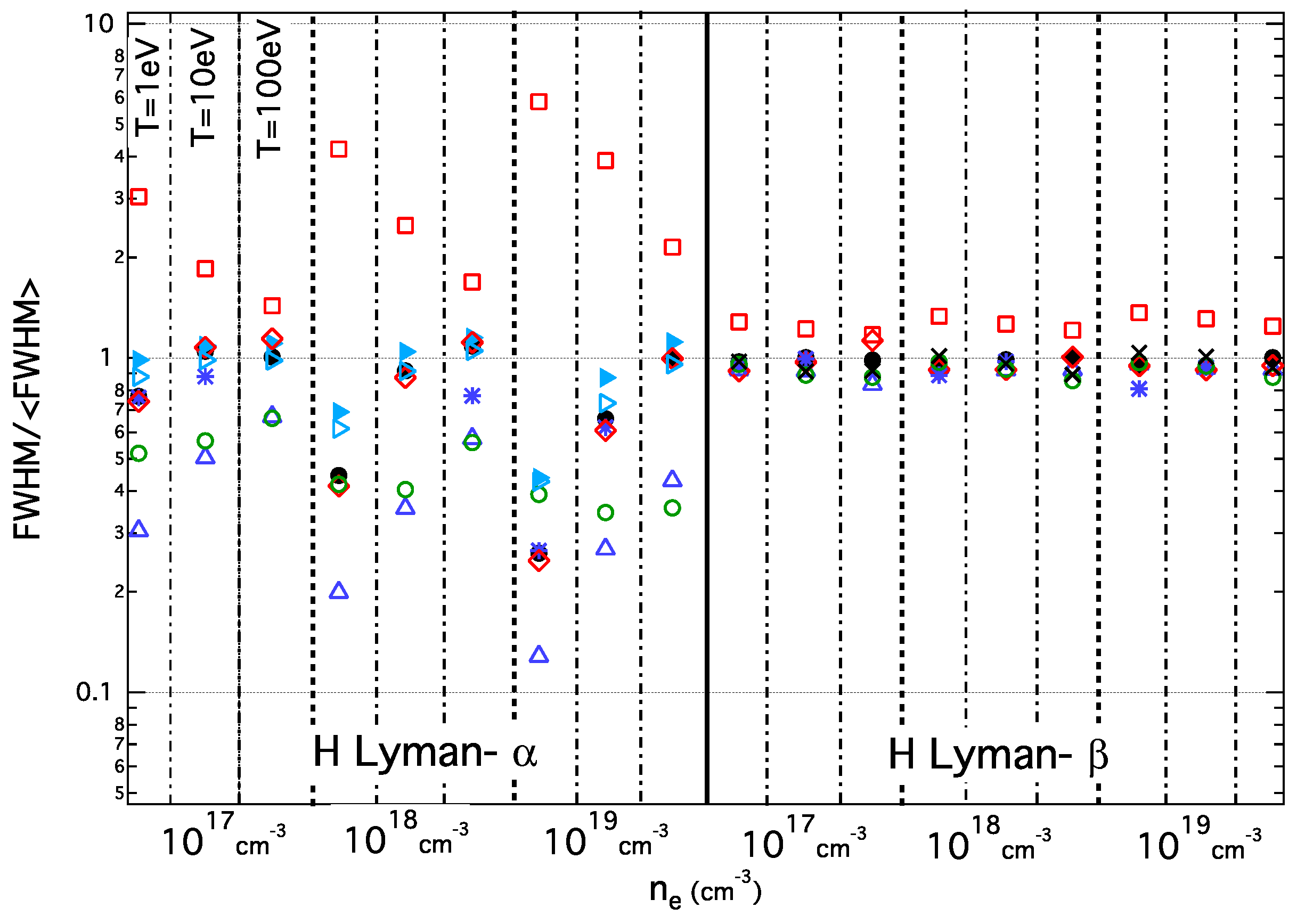
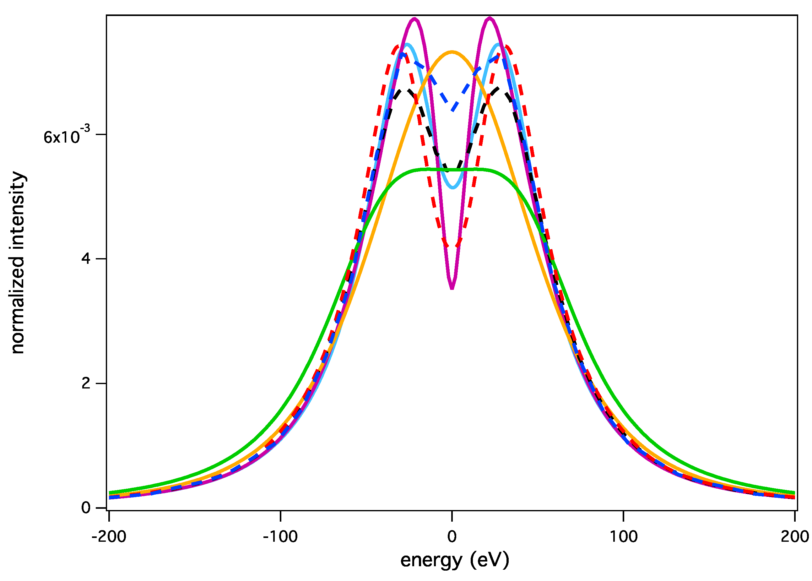
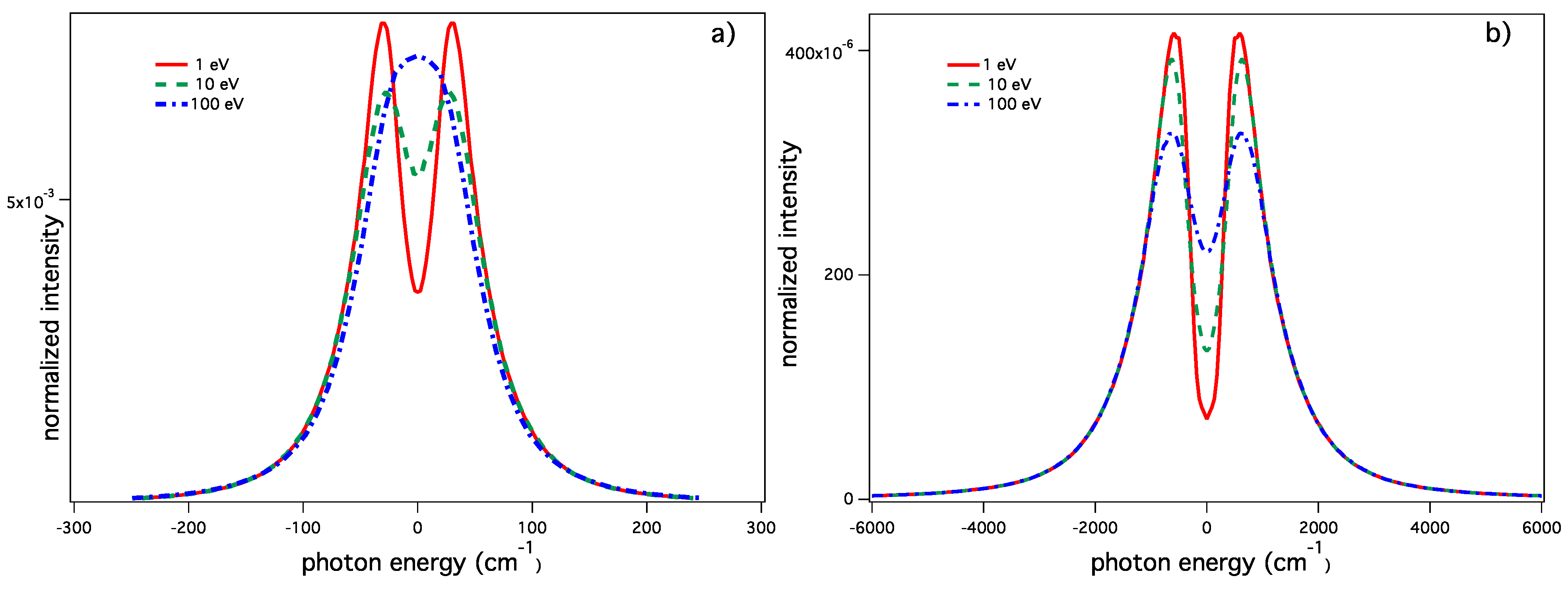
3.1.1. The Lyman-α Line


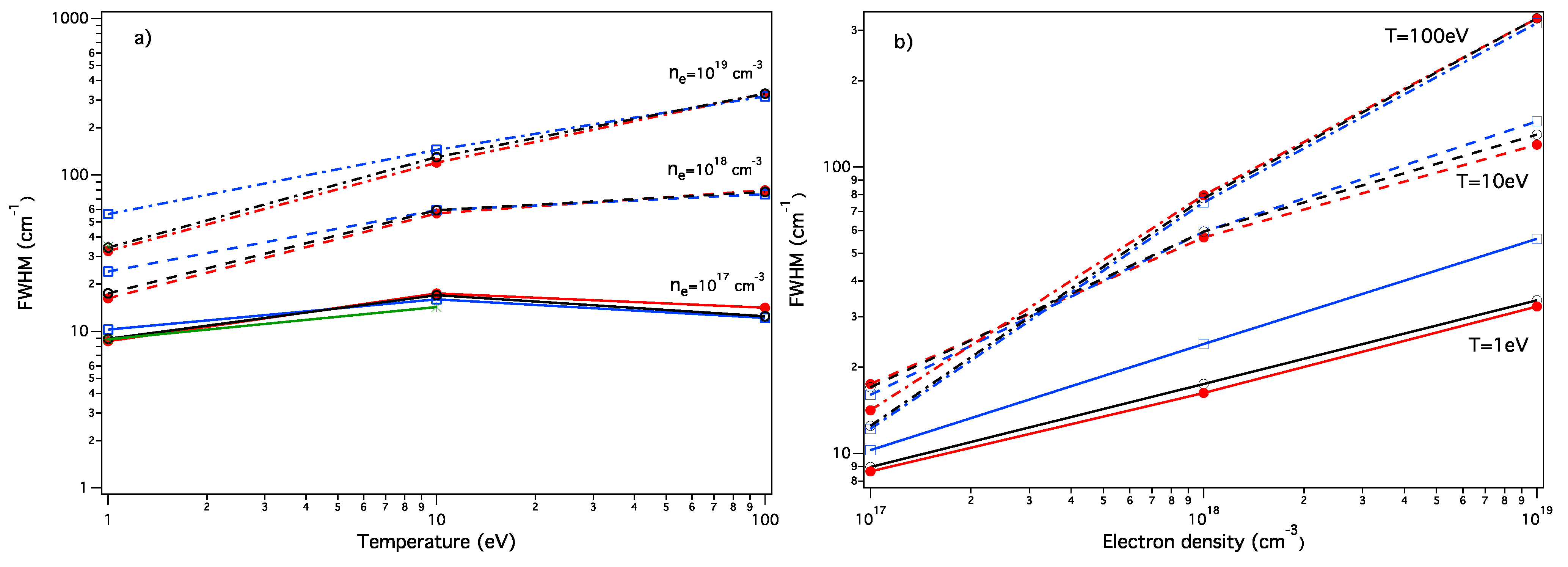
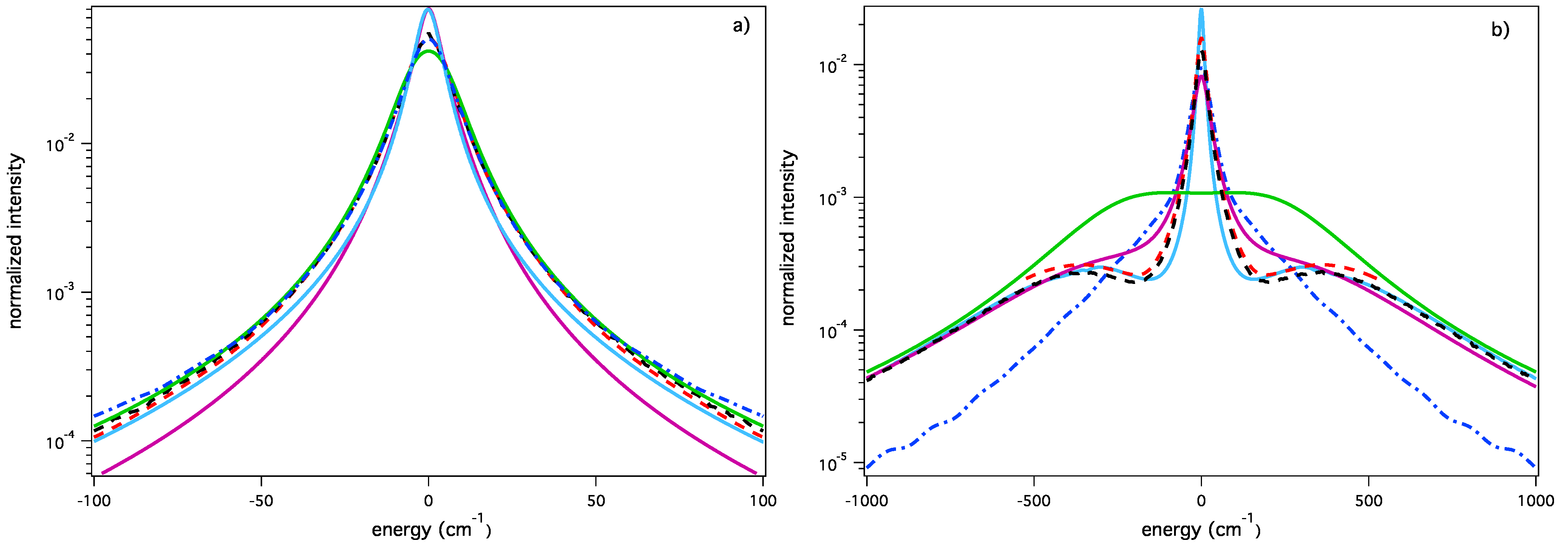
3.1.2. The Lyman-β Line


| T (eV) = | 1 | 10 | 100 |
| ER-simulation | 75 | 44 | 10 |
| SimU | 56 | 19 | 0 |
| Xenomorph | 56 | 14 | / |
| PPP | 70 | 31 | 0 |
| QuantSt.MMM | 71 | 55 | 32 |
| UTPP | 0.6 | 0.6 | 0 |
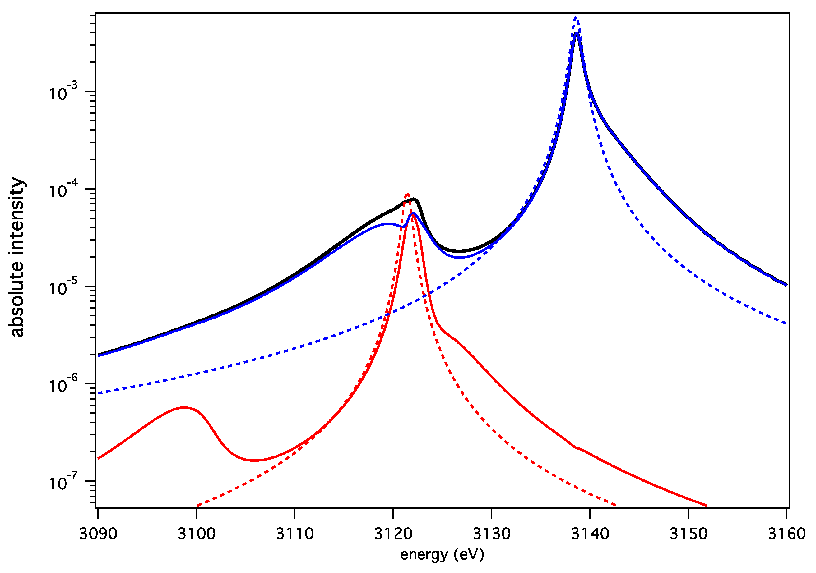
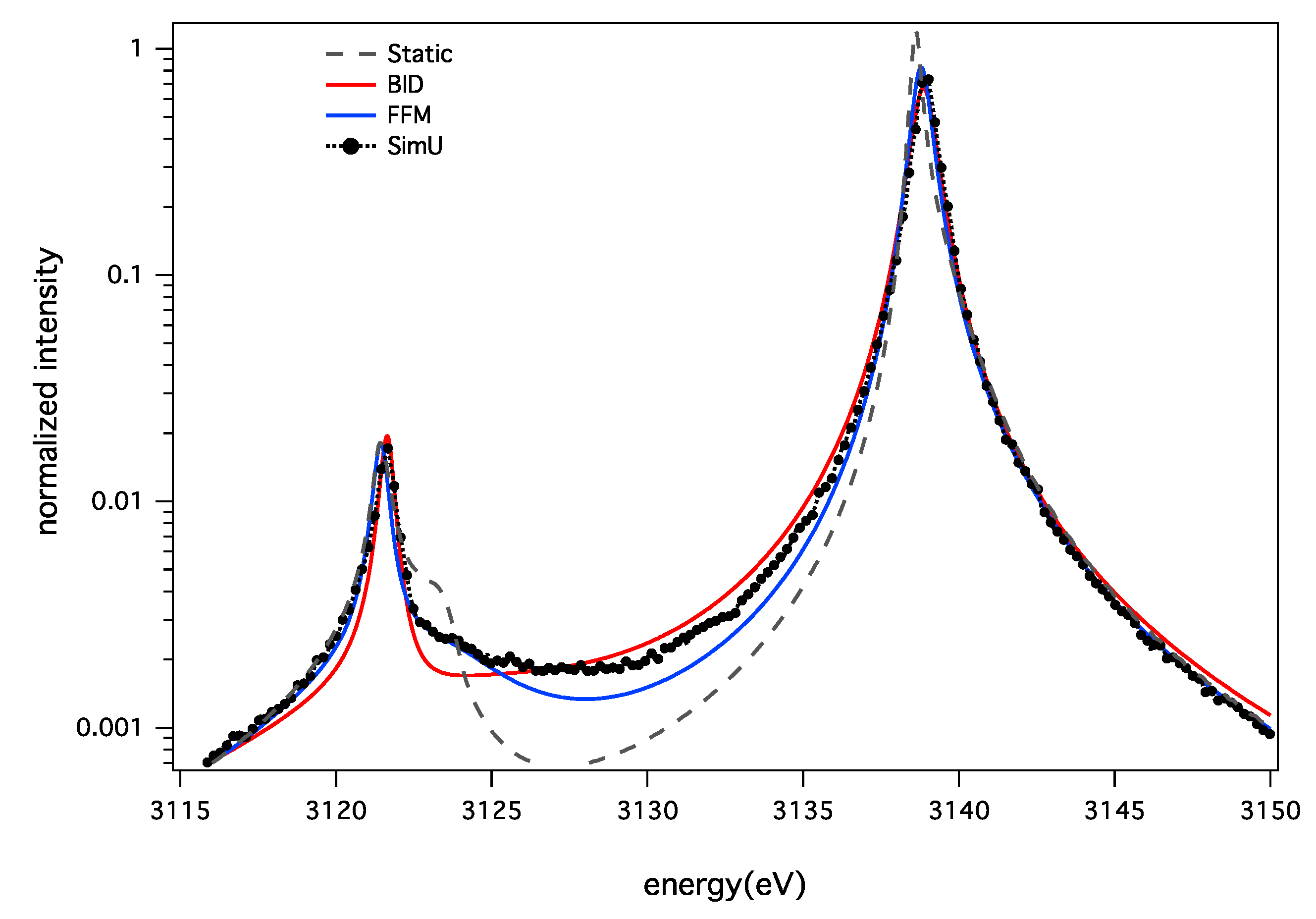
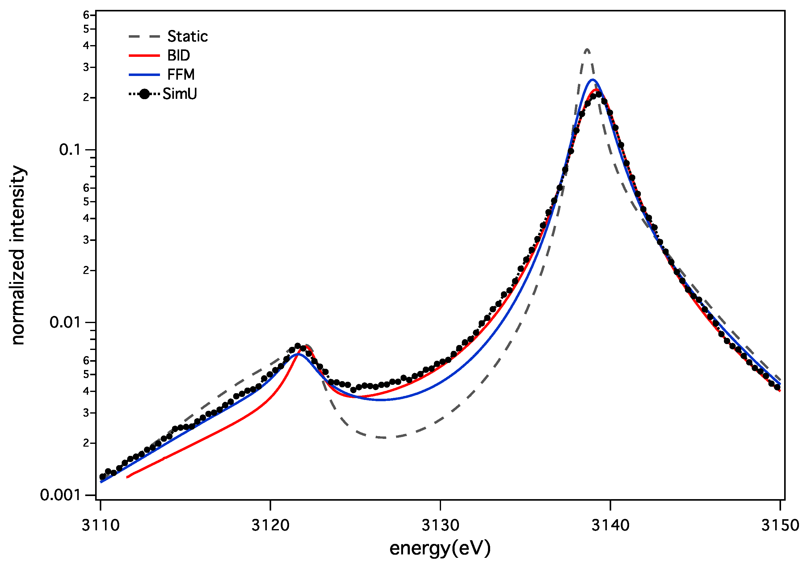
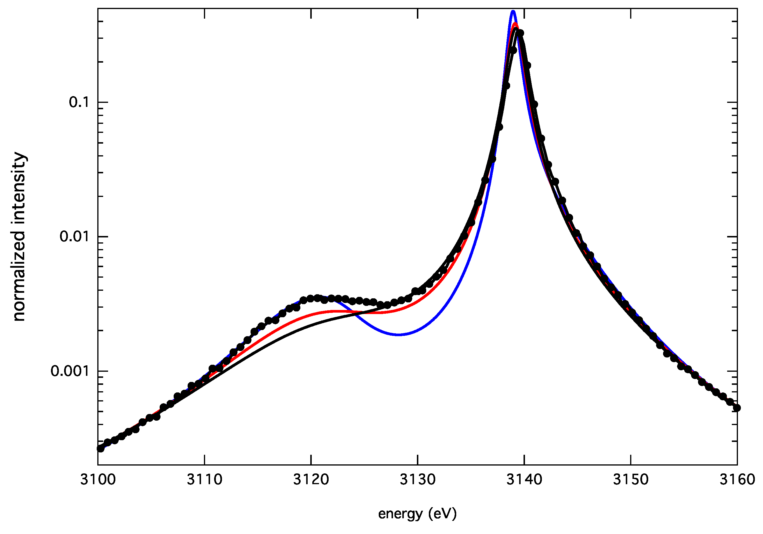
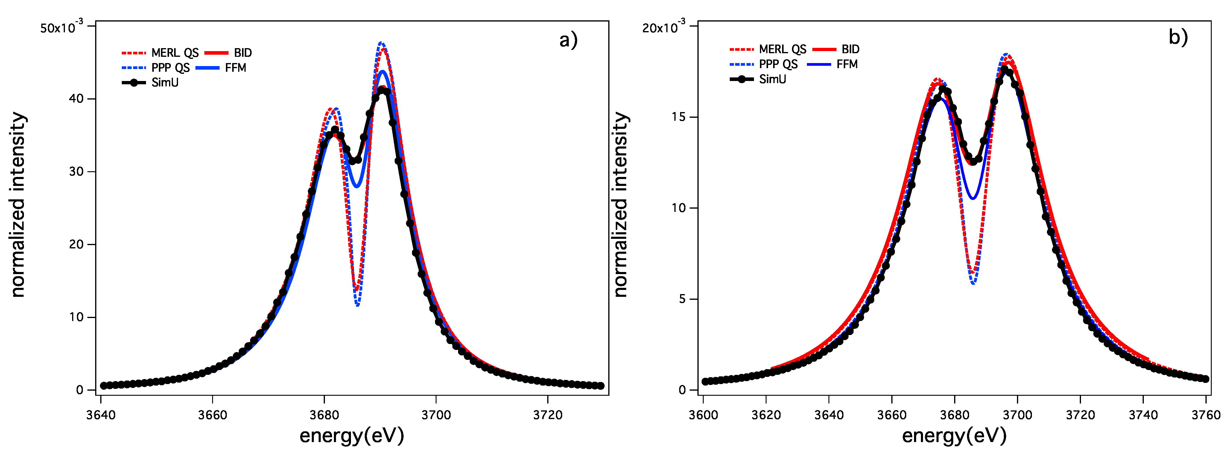
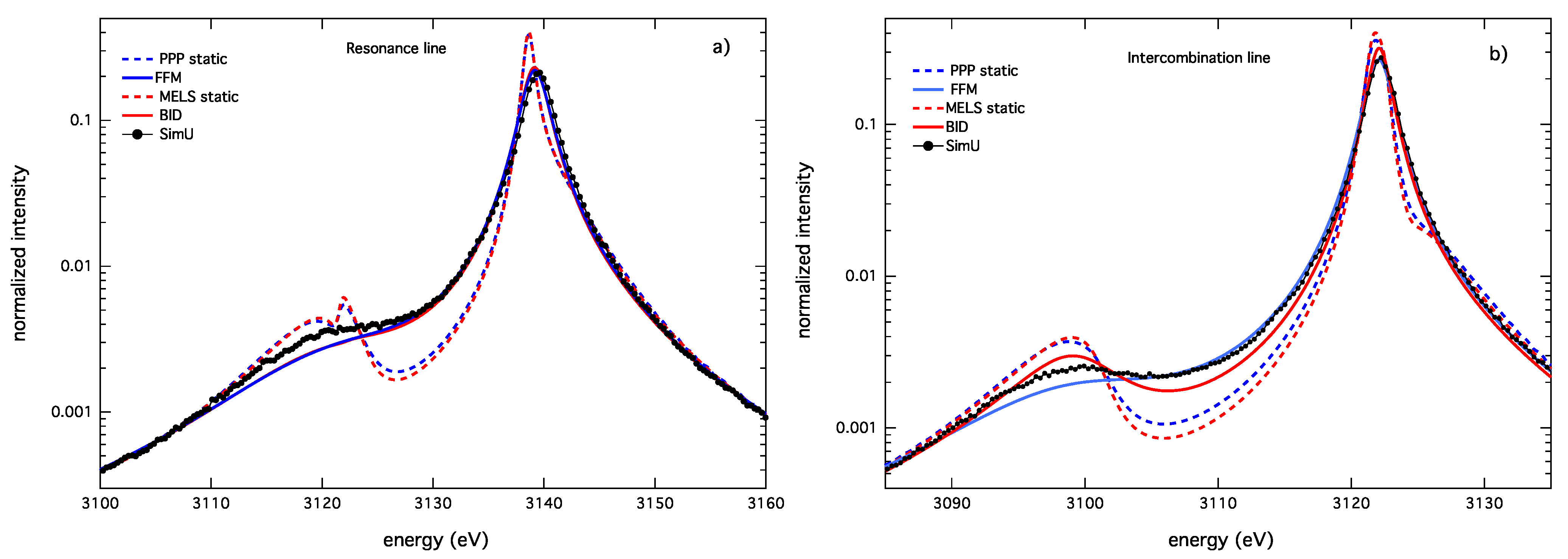
3.2. Argon He-α and He-β Lines


| Models | BID | FFM |
|---|---|---|
| cm | 58 | 57 |
| cm | 50 | 51 |
| cm | 47 | 48 |
4. Conclusions
Acknowledgments
Author Contributions
Conflicts of Interest
References
- Griem, H.R. Principles of Plasma Spectroscopy; Cambridge University Press: Cambridge, UK, 1997. [Google Scholar]
- Griem, H.R. Spectral Line Broadening by Plasmas; Academic Press: New York, NY, USA, 1974; ISBN 0-12-302850-7. [Google Scholar]
- Stambulchik, E.; Maron, Y. Plasma line broadening and computer simulations: A mini-review. High Energy Density Phys. 2010, 6, 9–14. [Google Scholar] [CrossRef]
- Calisti, A.; Mossé, C.; Ferri, S.; Talin, B.; Rosmej, F.; Bureyeva, L.A.; Lisitsa, V.S. Dynamic Stark broadening as the Dicke narrowing effect. Phys. Rev. E Stat. Nonlin. Soft Matter Phys. 2010, 81, 016406. [Google Scholar] [CrossRef]
- Stambulchik, E. Review of the 1st Spectral Line Shapes in Plasmas code comparison workshop. High Energy Density Phys. 2013, 9, 528–534. [Google Scholar] [CrossRef]
- Gigosos, M.A.; Gonzalez, M.A. Comment on “A study of ion-dynamics and correlation effects for spectral line broadening in plasmas: K-shell lines”. J. Quant. Spectrosc. Radiat. Transf. 2007, 105, 533–535. [Google Scholar] [CrossRef]
- Alexiou, S. Stark broadening of hydrogen lines in dense plasmas: Analysis of recent experiments. Phys. Rev. E Stat. Nonlin. Soft Matter Phys. 2005, 71, 066403. [Google Scholar] [CrossRef]
- Alexiou, S. Implementation of the Frequency Separation Technique in general lineshape codes. High Energy Density Phys. 2013, 9, 375–384. [Google Scholar] [CrossRef]
- Stambulchik, E.; Maron, Y. A study of ion-dynamics and correlation effects for spectral line broadening in plasma: K-shell lines. J. Quant. Spectrosc. Radiat. Transf. 2006, 99, 730–749. [Google Scholar] [CrossRef]
- Stambulchik, E.; Alexiou, S.; Griem, H.R.; Kepple, P.C. Stark broadening of high principal quantum number hydrogen Balmer lines in low-density laboratory plasmas. Phys. Rev. E Stat. Nonlin. Soft Matter Phys. 2007, 75, 016401. [Google Scholar] [CrossRef]
- Gomez, T.A.; Mancini, R.C.; Montgomery, M.H.; Winget, D.E. White dwarf line shape theory including ion dynamics and asymmetries. 2014. in preparation. [Google Scholar]
- Lorenzen, S. Comparative Study on Ion-Dynamics for Broadening of Lyman Lines in Dense hydrogen Plasmas. Contrib. Plasma Phys. 2013, 53, 368–374. [Google Scholar] [CrossRef]
- Stambulchik, E.; Maron, Y. Quasicontiguous frequency-fluctuation model for calculation of hydrogen and hydrogen-like Stark-broadened line shapes in plasmas. Phys. Rev. E Stat. Nonlin. Soft Matter Phys. 2013, 87, 053108. [Google Scholar] [CrossRef]
- Iglesias, C.A.; Vijay, S. Robust algorithm for computing quasi-static Stark broadening of spectral lines. High Energy Density Phys. 2010, 6, 399–405. [Google Scholar] [CrossRef]
- Woltz, L.A.; Hooper, C.F., Jr. Calculation of spectral line profiles of multielectron emitters in plasmas. Phys. Rev. A 1988, 38, 4766–4771. [Google Scholar] [CrossRef] [PubMed]
- Mancini, R.C.; Kilcrease, D.P.; Woltz, L.A.; Hooper, C.F. Calculational Aspects of the Stark Line Broadening of Multielectron Ions in Plasmas. Comput. Phys. Commun. 1991, 63, 314–322. [Google Scholar] [CrossRef]
- Calisti, A.; Khelfaoui, F.; Stamm, R.; Talin, B.; Lee, R.W. Model for the line shapes of complex ions in hot and dense plasmas. Phys. Rev. A 1990, 42, 5433–5440. [Google Scholar] [CrossRef] [PubMed]
- Alexiou, S.; Poquérusse, A. Standard line broadening impact theory for hydrogen including penetrating collisions. Phys. Rev. E Stat. Nonlin. Soft Matter Phys. 2005, 72, 046404. [Google Scholar] [CrossRef]
- Rosato, J.; Capes, H.; Stamm, R. Influence of correlated collisions on Stark-broadened lines in plasmas. Phys. Rev. E Stat. Nonlin. Soft Matter Phys. 2012, 86, 046407. [Google Scholar] [CrossRef]
- Boercker, D.B.; Iglesias, C.A.; Dufty, J.W. Radiative and transport properties of ions in strongly coupled plasmas. Phys. Rev. A 1987, 36, 2254–2264. [Google Scholar] [CrossRef] [PubMed]
- Talin, B.; Calisti, A.; Godbert, L.; Stamm, R.; Lee, R.W.; Klein, L. Frequency-fluctuation model for line shape calculations in plasma spectroscopy. Phys. Rev. A 1995, 51, 1918–1928. [Google Scholar] [CrossRef] [PubMed]
- Holtsmark, J. Über die Verbreiterung von Spektrallinien. Ann. Phys. 1919, 58, 577–630. [Google Scholar] [CrossRef]
- Iglesias, C.A.; Boercker, D.B.; Iglesias, C.A. Electric field distributions in strongly coupled plasmas. Phys. Rev. A 1985, 31, 1681–1686. [Google Scholar]
- Gigosos, M.A.; Gonzalez, M.A.; Cardeñoso, V. Computer simulated Balmer-alpha, -beta and -gamma Stark line profiles for non-equilibrium plasmas diagnostics. Spectrochim. Acta Part B 2003, 58, 1489–1504. [Google Scholar] [CrossRef]
- Gigosos, M.A.; Cardeñoso, V. New plasma diagnostics table of hydrogen Stark broadening including ion dynamics. J. Phys. B-At. Mol. Opt. Phys. 1996, 29, 4795–4838. [Google Scholar] [CrossRef]
- Hegerfeldt, G.; Kesting, V. Collision-time simulation technique for pressure-broadened spectral lines with applications to Ly-α. Phys. Rev. A 1988, 37, 1488–1496. [Google Scholar] [CrossRef] [PubMed]
- Filon, L.N.G. On a quadrature formula for trigonometric integrals. Proc. R. Soc. Edinb. 1928, 49, 38–47. [Google Scholar]
- Pfennig, H. On the Time-Evolution Operator in the Semiclassical Theory of Stark-Broadening of hydrogen Lines. J. Quant. Spectrosc. Radiat. Transf. 1972, 12, 821–837. [Google Scholar] [CrossRef]
- Lisitsa, V.S.; Sholin, G.V. Exact Solution of the Problem of the Broadening of the hydrogen Spectral Lines in the One-Electron Theory. Sov. J. Exp. Theor. Phys. 1972, 34, 484–489. [Google Scholar]
- Gigosos, M.A.; González, M.A. Calculations of the polarization spectrum by two-photon absorption in the hydrogen Lyman-α line. Phys. Rev. E Stat. Nonlin. Soft Matter Phys. 1998, 58, 4950–4959. [Google Scholar] [CrossRef]
- Djurović, S.; Ćiris̎an, M.; Demura, A.V.; Demchenko, G.V.; Nikolić, D.; Gigosos, M.A.; Gonzalez, M.Á. Measurements of Hβ Stark central asymmetry and its analysis through standard theory and computer simulations. Phys. Rev. E Stat. Nonlin. Soft Matter Phys. 2009, 79, 046402. [Google Scholar] [CrossRef] [PubMed]
- Frisch, U.; Brissaud, A. Theory of Stark broadening—I soluble scalar model as a test. J. Quant. Spectrosc. Radiat. Transf. 1971, 11, 1753–1766. [Google Scholar] [CrossRef]
- Frisch, U.; Brissaud, A. Theory of Stark broadening—II exact line profile with model microfield. J. Quant. Spectrosc. Radiat. Transf. 1971, 11, 1767–1783. [Google Scholar]
- Günter, S.; Hitzschke, L.; Röpke, G. Hydrogen spectral lines with the inclusion of dense-plasma effects. Phys. Rev. A 1991, 44, 6834–6844. [Google Scholar] [CrossRef] [PubMed]
- Lorenzen, S.; Omar, B.; Zammit, M.C.; Fursa, D.V.; Bray, I. Plasma pressure broadening for few-electron emitters including strong electron collisions within a quantum-statistical theory. Phys. Rev. E Stat. Nonlin. Soft Matter Phys. 2014, 89, 023106. [Google Scholar] [CrossRef]
- Dufty, J.W. Spectral Lines Shapes; Wende, B., Ed.; De Gruyter: New York, NY, USA, 1981. [Google Scholar]
- Stambulchik, E.; Maron, Y. Stark effect of high-n hydrogen-like transitions: Quasi-contiguous approximation. J. Phys. B-At. Mol. Opt. Phys. 2008, 41, 095703. [Google Scholar] [CrossRef]
- Mossé, C.; Calisti, A.; Stamm, R.; Talin, B.; Lee, R.W.; Klein, L. Redistribution of resonance radiation in hot and dense plasmas Phys. Rev. A 1999, 60, 1005–1014. [Google Scholar] [CrossRef]
- Iglesias, C. Efficient algorithms for stochastic Stark-profile calculations. High Energy Density Phys. 2013, 9, 209–221. [Google Scholar] [CrossRef]
- Rosato, J.; Reiter, D.; Kotov, V.; Marandet, Y.; Capes, H.; Godbert-Mouret, L.; Koubiti, M.; Stamm, R. Progress on radiative transfer modelling in optically thick divertor plasmas. Contrib. Plasma Phys. 2010, 50, 398–403. [Google Scholar] [CrossRef]
- Rosato, J.; Capes, H.; Stamm, R. Divergence of the Stark collision operator at large impact parameters in plasma spectroscopy models. Phys. Rev. E Stat. Nonlin. Soft Matter Phys. 2013, 88, 035101:1–035101:3. [Google Scholar] [CrossRef]
- Rosato, J.; Capes, H.; Stamm, R. Ideal Coulomb plasma approximation in line shape models: Problematic issues. Atoms 2014, 2(2), 277–298. [Google Scholar] [CrossRef]
- Lisitsa, V. Private communication.
- Calisti, A.; Demura, A.V.; Gigosos, M.A.; González-Herrero, D.; Iglesias, C.A.; Lisitsa, V.S.; Stambulchik, E. Influence of Microfield Directionality on Line Shapes. Atoms 2014, 2, 259–276. [Google Scholar] [CrossRef]
- Chung, H.-K.; Lee, R.W. Application of NLTE population kinetics. High Energy Density Phys. 2009, 5, 1–14. [Google Scholar] [CrossRef]
- Woolsey, N.C.; Hammel, B.A.; Keane, C.J.; Asfaw, A.; Back, C.A.; Moreno, J.C.; Nash, J.K.; Calisti, A.; Mossé, C.; Stamm, R.; et al. Evolution of electron temperature and electron density in indirectly driven spherical implosions. Phys. Rev. E Stat. Nonlin. Soft Matter Phys. 1996, 56, 2314. [Google Scholar] [CrossRef]
- Haynes, D.A.; Garber, D.T.; Hooper, C.F.; Mancini, R.C.; Lee, Y.T.; Bradley, D.K.; Delettrez, J.; Epstein, R.; Jaanimagi, P.A. Effects of ion dynamics and opacity on Stark-broadened argon line profiles. Phys. Rev. E Stat. Nonlin. Soft Matter Phys. 1996, 53, 1042–1050. [Google Scholar] [CrossRef]
- Mancini, R.C.; Iglesias, C.A.; Ferri, A.; Calisti, S.; Florido, R. The effects of improved satellite line shapes on the argon Heβ spectral feature. High Energy Density Phys. 2013, 9, 731–736. [Google Scholar] [CrossRef]
© 2014 by the authors; licensee MDPI, Basel, Switzerland. This article is an open access article distributed under the terms and conditions of the Creative Commons Attribution license (http://creativecommons.org/licenses/by/3.0/).
Share and Cite
Ferri, S.; Calisti, A.; Mossé, C.; Rosato, J.; Talin, B.; Alexiou, S.; Gigosos, M.A.; González, M.A.; González-Herrero, D.; Lara, N.; et al. Ion Dynamics Effect on Stark-Broadened Line Shapes: A Cross-Comparison of Various Models. Atoms 2014, 2, 299-318. https://doi.org/10.3390/atoms2030299
Ferri S, Calisti A, Mossé C, Rosato J, Talin B, Alexiou S, Gigosos MA, González MA, González-Herrero D, Lara N, et al. Ion Dynamics Effect on Stark-Broadened Line Shapes: A Cross-Comparison of Various Models. Atoms. 2014; 2(3):299-318. https://doi.org/10.3390/atoms2030299
Chicago/Turabian StyleFerri, Sandrine, Annette Calisti, Caroline Mossé, Joël Rosato, Bernard Talin, Spiros Alexiou, Marco A. Gigosos, Manuel A. González, Diego González-Herrero, Natividad Lara, and et al. 2014. "Ion Dynamics Effect on Stark-Broadened Line Shapes: A Cross-Comparison of Various Models" Atoms 2, no. 3: 299-318. https://doi.org/10.3390/atoms2030299
APA StyleFerri, S., Calisti, A., Mossé, C., Rosato, J., Talin, B., Alexiou, S., Gigosos, M. A., González, M. A., González-Herrero, D., Lara, N., Gomez, T., Iglesias, C., Lorenzen, S., Mancini, R. C., & Stambulchik, E. (2014). Ion Dynamics Effect on Stark-Broadened Line Shapes: A Cross-Comparison of Various Models. Atoms, 2(3), 299-318. https://doi.org/10.3390/atoms2030299