Abstract
Positron scattering by beryllium atoms in the low-energy range (≤4.0 eV) was studied within ab initio and semiempirical frameworks. When interpreting the static dipole polarizability and the scattering length as representative quantities of the target and positron–atom correlations, the scattering observables obtained in the ab initio calculation were extrapolated by applying a semiempirical approach. Our results ratify previous ones, since no Ramsauer minimum structures or shape resonances were found in the cross sections. The presence of a () bound state was also identified as a function of the dipole polarizability.
Keywords:
elastic scattering; positron scattering; ab initio; semiempirical potentials; scattering length; polarizability; many-body PACS:
34.80.Bm; 34.80.-i
1. Introduction
Low-energy positron scattering by atoms and molecules forms an interesting source of information about the interaction dynamics of antielectrons with ordinary matter [1]. In particular, a considerable challenge is present in the low-energy region, where the correlation–polarization effects are important and high-energy standard approaches, such as the first Born approximation and its variations, are not valid.
Specifically, the positron scattering by the alkaline earth atoms has been the subject of investigations from time to time. These chemical species are closed shell-like systems, for which the theoretical procedures are similar to those found in calculations with noble gas atoms.
As far as we know, the first specific calculation of low-energy positron–Be scattering was that reported by Kurtz and Jordan [2] in the early 1980s. They applied the Harris method [3] while considering an ad hoc polarization potential. A Ramsauer minimum at 1.6 eV was found in the s-wave phase shift, but it was obscured in the total cross section due to the large contributions from the p and d waves near this energy. This peculiarity was also observed in positron scattering by rare gas atoms [4]. Interestingly, a virtual state was found from the identification of a pole in the S matrix on the imaginary k axis [2].
In 1993, Szmytkowski applied the relativistic polarized orbital method to investigate the problem [5]. Unlike in the previous calculations of Kurtz and Jordan [2], the polarization potential was calculated in a fully ab initio framework by solving the coupled Dirac–Hartree–Fock equations. The large positive value that was found for the scattering length suggested that the scattering potential could support a weakly bound state.
The existence of a bound state was theoretically established in 1998 in a fixed-core stochastic variational method (FCSVM) calculation performed by Ryzhikh et al. [6]. Afterward, the weak binding energy (0.00278 Hartree) found in the FCSVM was used by Bromley et al. [7] to tune different semiempirical potentials and investigate low-energy positron–Be elastic scattering.
The Ramsauer effect in electron and positron scattering by Be was examined by Reid and Wadehra [8]. They used an energy-dependent correlation–polarization model potential, and no Ramsauer effect was found for positrons.
More recently, Poveda et al. [9] applied an ab initio local model potential based on a finite nuclear mass correction. They found an interesting structure in the elastic cross section around 1 eV due to the p-wave scattering associated with a frustrated shape resonance. In particular, the existence of a bound state was verified through a direct calculation from the potential curve.
Therefore, one might conclude that there is a weak bound state, and that the Ramsauer minima and shape resonances are absent in the elastic cross section.
In this work, we investigated the low-energy positron–Be scattering while taking a well-established many-body ab initio (AI) method as a reference for the positron–target correlation. Then, by using a semiempirical (SEMP) approach, we extrapolated how the scattering observables varied according to target polarizability.
The AI calculations were performed with the Schwinger multichannel method (SMC) for positrons [10], which we have already applied to investigate the elastic scattering and rotational excitation of H2 [11], Li2 [12], and N2 [13] as a result of positron impact. Curiously, as far as we know, helium is the only atomic target that has been studied with this method [14,15]. Since beryllium has only four electrons and a simple closed-shell electronic structure, it is the next system in the order of complexity and an excellent candidate for AI many-body calculations.
In the absence of any experimental data on this system,1 an AI investigation is rather welcome. Every theoretical methodology is built from an interaction model that is composed of a description of the target and the short- and long-range electron–positron correlations. From an AI calculation, it is expected that the results will be as accurate as those of the interaction model adopted. If the physics of the problem are correctly described, such calculations are able to accurately predict what should be experimentally observed. A field of research that illustrates this reasoning is the study of the polarizabilities of atoms, molecules, and clusters [17].
In the particular context of positron–atom scattering, although it is possible to control some aspects (basis set size, representation of scattering orbitals, representation of target state, et cetera), SMC calculations provide parameter-free answers to the problem under investigation. However, the computational cost and intrinsic complexity of a many-body calculation prohibit a study on how the cross sections vary with relevant target properties. Semiempirical methods, on the other hand, depend on how the model parameters are calibrated, but, in general, they provide information regarding the relevant variables in the description of the phenomenon, and they are mainly used to identify validation intervals of the physical quantities involved with simple calculations.
With these arguments, the objectives of this work are to find out what the many-body AI calculation with the SMC predicts for positron–Be scattering—more precisely, the phase shifts, scattering length, and elastic cross section—and then develop an extrapolation scheme based on physical grounds to investigate how the scattering observables vary depending on the polarizability of the target.
This paper is organized as follows: In Section 2, we describe the methods and computational procedures; in Section 3, we present the results obtained, with an emphasis on the analysis of possible scattering structures. Finally, in Section 4, we state our conclusions. Unless otherwise stated, we use atomic units throughout the text.
2. Methods and Procedures
2.1. Ab Initio Calculations
The AI calculations were performed with the SMC. The method was originally presented by Germano and Lima [10] and was applied to several molecular systems over time [18,19,20,21]. A complete description of the method can be found in [11,15], and in this work, we will provide only the main methodological elements.
Taking as the positron coordinate and as the coordinates for the electrons, the scattering wavefunction for the positron–atom system is written as
where forms a trial basis set. In this equation, denotes the HF ground-state wavefunction of the target () and the excited states (). The term represents the positron scattering orbitals—in this case, these are taken as the orbitals coming from the SCF calculation.
Considering the functional variation of the amplitude according to the Schwinger variational principle with respect to the coefficients , we get the working expression for the body–frame scattering amplitude:
with
In the equation above, is a solution of the unperturbed Hamiltonian (molecular Hamiltonian plus the kinetic energy operator for the incident positron); each Latin label compactly denotes , and P and Q are projectors onto energetically open and closed states of the target. The term V is the many-body electrostatic positron–target potential, is the total energy minus the scattering Hamiltonian, and is the projected Green function, which is written in this way in order to avoid the calculation of the target continuum states present in the free-particle Green function .
The initial input used in a standard SMC calculation is a set of Cartesian Gaussian functions (CGFs). This set is then used to generate the atomic ground-state wavefunction and the excited-state determinants. The drawback comes from the dependence of the cross sections on the CGF set that is elected to represent the target and the positron scattering orbitals [15,22].
The initial criterion for the selection of a basis set is the description of basic atomic properties, such as the ground-state energy and dipole polarizability. For practical applications of the SMC, we additionally consider the criteria described in [11,13], which, briefly speaking, verify if the basis is consistent with the first Born approximation and exhibit convergence between the methods used to compute the Green function.
For this work, we chose the one listed in Table 1, which was taken from [23] and augmented with s, p, and d functions. The energy obtained in the SCF calculation was Hartree, which presents a good agreement with the theoretical and experimental values [24,25]. For this basis set, we found the dipole polarizability of , which was computed with the GAMESS quantum chemistry package [26] by using a finite field approach. This value is in agreement with those given by Maroulis and Thakkar [27], who provided and for the two basis sets considered in their investigation at the SCF level of approximation.

Table 1.
Basis set of Cartesian Gaussian functions (CGFs) considered to describe the ground state of the Be atom and the positron scattering orbitals in this work. The CGF core was extracted from [23], and functions were added to obtain 15 of each kind. All functions are uncontracted.
2.2. Connecting Polarization, Correlation, and Scattering Length
It is well known that low-energy positron–atom cross sections are determined by the balance between static repulsive interactions and the attractive correlation–polarization ones. From perturbation theory, the asymptotic form of the potential (to the second order) is known as [28]:
where is the static dipole polarizability of the target. One concern, if not the major problem in the field, is the description of the positron–target correlation effects. These effects compete with the electrostatic effects when the positron gets close and penetrates the atomic cloud.
In model potential approaches, the correlation effects are generally modeled as if the positron distorts a gas of electrons as it superposes to the electronic cloud [29]. The disadvantage of this approach lies in the way that the asymptotic polarization potential (Equation (4)) is connected with the correlation potential. For practical purposes, the correlation and polarization potentials are piecewise connected at the point at which they cross each other for the first time [29,30]. In the SMC, the correlation–polarization effects are treated in a full many-body AI way through virtual excitations of the target. This standard of excellence demands its price: the scattering observables depend on the description adopted for the target and, mainly, on how the interaction model is assumed to describe the positron–target correlations. Once a CGF basis set is selected for the calculation (as discussed in [11,13]), this methodology is non-functional for the study of how the scattering observables change as the target or interaction parameters vary. This kind of investigation is better performed by using model or semiempirical approaches.
In the SMC, the target is described by using an HF wavefunction. This implies that the target electronic correlation is described at the SCF level. According to Table 3 of Maroulis and Thakkar [27], when electronic correlation is taken into account, the dipole polarizability goes to ≈37.0 a, i.e., ≈19% lower in magnitude than the SCF value of 45.6 a. From the point of view of positron scattering, this means that an SCF polarization such as that considered here provides an attractive asymptotic component of the potential that is deeper than the one that should be found if the target wavefunction used for scattering calculations considers the electronic correlation beyond, regardless of the SCF level.
At this point, the question that we wish to answer is the following: Taking the SMC correlation as a reference, how would the scattering parameters predicted by this method vary if a more sophisticated target electronic correlation was considered?
From a pragmatic point of view, the target correlation manifests in the value of , while the the intrinsic positron–target correlation of the SMC manifests at the scattering at zero energy, i.e., in the value of the scattering length A. So, if the function and the incorporation of the correlation is somehow known, then, this question can be answered.
Fortunately, this problem has already been tackled by Szmytkowski [31,32]. Assuming that the interaction potential has the form
where is the short-range component of the interaction, which is taken here as the positron–atom electrostatic potential, the scattering length A as a function of the polarizability is given by
where , and is the scattering length associated with the short-range component of the potential.
To find how A varies with in Equation (6), we adopted a similar procedure when studying the same problem for positron–Ar [4]. In practice, we need to determine the parameter R. Defining the dimensionless variables , , and , we get a transcendental equation:
The input values considered were , , and , which are, respectively, the dipole polarizability and the scattering lengths obtained with the SMC with and without polarization. The numerical solution of this equation provided or .
In what follows, we assume that:
- (1)
- is representative of the positron–target correlation of the SMC, and from now on, it will be considered a fixed value;
- (2)
- is representative of the electronic correlation of the target as considered in the SMC.
Figure 1 shows the plot of the scattering length A as a function of as given by Equation (6) in order to reproduce the scattering length obtained with the SMC. The range of values for goes from 37 to [27], but a larger range was considered in order to observe the change in sign of the scattering length for . Physically, this means that a virtual state turns into a bound state for , which, interestingly, is slightly below the lowest value for foreseen in the calculations of Maroulis and Thakkar [27].
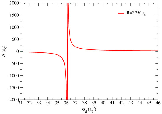
Figure 1.
Scattering length A as a function of the dipole polarizability according to Equation (6). The curve was obtained with in order to reproduce the scattering length obtained with the SMC.
2.3. Semiempirical Approach
Once the variation of A with is determined, we investigate the variation of the scattering observables for positron–Be by applying a semiempirical model [4,33,34,35]. The positron–atom scattering problem is treated by using the following single-body Hamiltonian:
where the first term represents the kinetic energy of the positron, represents the electrostatic positron–atom interaction that was calculated from the same CGFs as those considered in the SMC calculations, and the polarization potential, in turn, is taken as
where is an adjustable parameter. As expected, the values of were adjusted to reproduce the scattering lengths as a function of , as predicted from Equation (6). These values are shown in Table 2 for representative values of .
Table 2.
Table for the polarizabilities and scattering lengths for the semiempirical calculations.
In order to visualize the confidence level of the model, in Figure 2, we show the phase shifts computed from the scattering amplitude of the SMC (Equation (2)) and those obtained from the semiempirical calculation (; ). As we can see, some small discrepancies are seen in the p () and d () waves for energies above 1 eV, while the s wave () is very well described. There is nothing surprising in the quality of this fitting because the criterion for fixing the parameter was defined to privilege s-wave scattering, which is dominant at low energies. In spite of these small discrepancies in the p and d waves, we proceed in the exploration of the results because, as we can see, the model managed to capture the essence of the physics in question. The effects of the p and d deviations in the elastic cross section will be discussed in Figure 4.
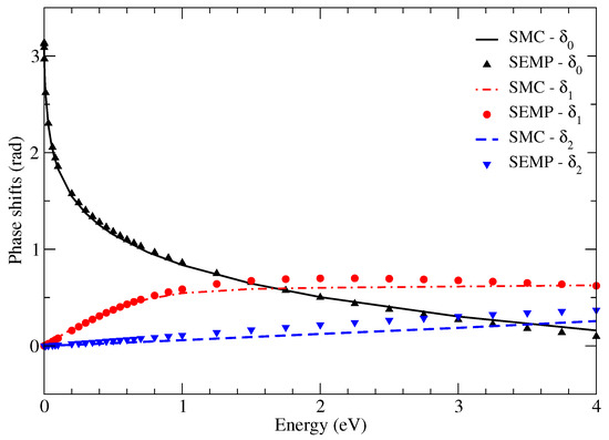
Figure 2.
Phase shifts in radians as a function of the impact energy in eV computed with the SMC and the semiempirical model (SEMP) according to the SMC reference data: a, a, and a (see the first line of Table 2). , , and denote the s-, p-, and d-wave phase shifts, respectively. Some small discrepancies are seen for the p and d waves for energies above 1 eV, while the s wave is well described, as expected.
2.4. A Final Remark
As a final remark to close this section, over the last few years, we have studied how polarization terms of an order higher than affect positron–atom [36] and positron–molecule [37] scattering by using semiempirical [34] and model potentials [38]. Recently, in an investigation on positron scattering by F2 molecules [39], we showed that the SMC provides similar cross sections to those calculated with model correlations when only the term is considered. Consequently, in this work, we focus on the study of cross sections while considering exclusively the effect of the polarization. Hyperpolarization effects will be addressed in a future article.
3. Results and Discussion
With the methodology defined in the previous section, we now proceed to the analysis of the results. The first set of scattering observables to be analyzed are the phase shifts. These are plotted in Figure 3 and Figure 4 for the s and p waves, respectively, for the set of polarizabilities in Table 2 as a function of the impact energy in eV.
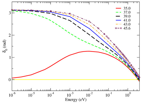
Figure 3.
S-wave phase shifts for positron–Be as a function of the dipole polarizability . The values of are given in . A yellow line marks in order to identify the suppression of the s-wave cross section.
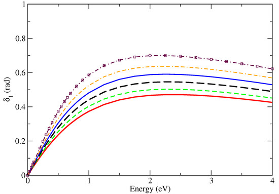
Figure 4.
The same as Figure 3, but for the p wave. Note that no shape resonance is found for any value of . The legends are the same.
In Figure 3, we see that for , starts from zero and quickly grows with the energy, indicating that the potential is on the verge of forming an s-wave bound state. For , the scattering length changes sign (see Figure 1 and Table 2), and the bound state is formed. It is interesting to observe that according to the correlation model adopted here, a measure of would indicate whether a bound state exists. According to Levinson’s theorem, at zero energy, we shall find . It is interesting to observe that crosses the zero value for energies next to 4 eV. In practice, this means that no noticeable Ramsauer minimum structure will appear in the elastic cross section, since, at this energy, the other partial waves fill the background. The graph of the p-wave phase shift in Figure 4, on the other hand, shows no bound-state structure or any sign of shape resonance.
Now that the phase shifts have been shown, we look at the cross sections in Figure 5. In the upper panel, we can visualize how the cross sections vary with . Clearly, the cross sections exhibit the typical energy dependence observed in other atomic systems, such as those of Ar, Kr, and Xe [34], and they grow in magnitude with the value of for a fixed energy. When analyzing these graphs, it is important to be aware that the ionization potential of Be is 9.3 eV [40], which implies a threshold for positronium formation of 2.5 eV. In addition, the threshold for the electronic excitation 1s22s2 (1S) → 1s22s2p (1P0) is 2.7 eV [41]. Therefore, the scattering is genuinely elastic for impact energies below ≈2.5 eV.
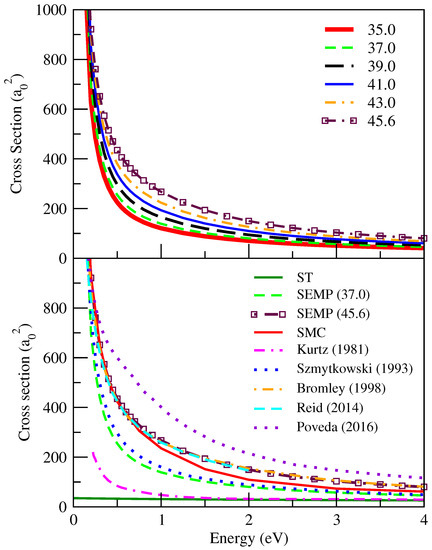
Figure 5.
Elastic integral cross sections for positron–Be. Upper panel: cross sections as a function of given in . Bottom panel: this work compared to previous ones. (Refs. [2,5,7,8,9]).
In the bottom panel, we see how the cross sections computed in this work compare to the previous ones reported in the literature. For the sake of completeness, in Table 3, we show the respective polarizabilities and scattering lengths. We first pay attention to the model calculation of Kurtz and Jordan [2]. These authors worked with a correlation–polarization potential similar to that found in Equation (5), but with a criterion for defining R associated with the angular momentum barrier. Thus, a different R was adopted for each partial wave. As we can see, their results are very similar to those computed in the static (ST) approximation, which suggests that the polarization that they considered was underestimated. The results obtained within the semiempirical approach for (SEMP (37.0)) and (SEMP (45.6)) are shown, in addition to the results directly produced by the SMC. A small discrepancy is seen between the SMC and SEMP (45.6) for energies above 1 eV, as expected from the phase shifts in Figure 2.
Table 3.
Scattering lengths A and dipole polarizabilities considered for positron–Be according to previous works. All values are in atomic units.
The AI results that Szmytkowski [5] obtained with the relativistic polarized orbital method are quite close to ours for in the range of 0.25 to 4.0 eV. Nevertheless, there is no agreement in the values for the scattering lengths, which indicates that our s-wave phase shift is appreciably different from his. This is expected because the potentials are distinct. The semiempirical and model potential results of Bromley et al. [7] and Reid and Wadehra [8] are practically equal and coincide with our semiempirical ones for . Finally, the AI cross section of Poveda et al. [9] clearly shows the higher magnitude when compared to all other results.
4. Conclusions
Low-energy positron scattering by beryllium was primarily studied in the ab initio context. Specifically, the calculations were performed with the Schwinger multichannel method, a variational treatment that incorporates the many-body character of the problem. In order to understand how the scattering observables vary with the inherent correlation schemes incorporated in this method, we took the static dipole polarizability and the scattering length A as the main parameters that carry information on the target and positron–atom correlations. Through the calculation of A as a function of based on Szmytkowski’s theory, we extrapolated the scattering observables predicted in the ab initio calculation by applying a semiempirical approach. According to the correlation model adopted here, a measure of would indicate whether a bound state exists.
Our results corroborate the findings of previous investigations, i.e., a () bound state was found for , and no Ramsauer minimum or shape resonances were present in the cross sections. Phase shifts and elastic cross sections were reported as a function of in the range of values discussed in the work of Maroulis and Thakkar [27].
Future perspectives are the extension of this investigation to study the effect of higher-order polarization effects in the low-energy cross sections—a point that still needs to be better understood in the context of alkaline earth metals—and to improve the description of the correlation effects within the SMC.
Author Contributions
Conceptualization, M.V.B., W.T. and F.A.; methodology, M.V.B., W.T. and F.A.; writing—original draft preparation, F.A.; writing—review and editing, M.V.B., W.T. and F.A. All authors have read and agreed to the published version of the manuscript.
Funding
This research received no external funding.
Data Availability Statement
The data of this research is available upon request to the authors.
Acknowledgments
M.V. Barp would like to thank the Conselho Nacional de Desenvolvimento Científico e Tecnológico for the financial support. M.V. Barp, F. Arretche, and W. Tenfen would like to thank the Programa de Pós-Graduação em Física of Universidade Federal de Santa Catarina and Universidade Federal de Pelotas for the support.
Conflicts of Interest
The authors declare no conflict of interest.
Abbreviations
The following abbreviations are used in this manuscript:
| HF | Hartree–Fock |
| SMC | Schwinger multichannel method |
| CGF | Cartesian Gaussian functions |
| FCSVM | Fixed-core stochastic variational method |
| ST | Static |
| AI | Ab initio |
| SEMP | Semiempirical |
| MP | Model potential |
| SCF | Self-consistent field |
| GAMESS | General atomic and molecular electronic structure system |
| ICS | Integral cross section |
Note
| 1 | With regard to experimental data for alkaline earth atoms, total cross section data are available for Mg [16]. |
References
- Surko, C.M.; Gribakin, G.; Buckman, S.J. Low-energy positron interactions with atoms and molecules. J. Phys. B At. Mol. Opt. Phys. 2005, 38, R57. [Google Scholar] [CrossRef]
- Kurtz, H.; Jordan, K. Theoretical study of low-energy electron and positron scattering on Be, Mg and Ca. J. Phys. B At. Mol. Phys. 1981, 14, 4361. [Google Scholar] [CrossRef]
- Harris, F.E. Expansion approach to scattering. Phys. Rev. Lett. 1967, 19, 173. [Google Scholar] [CrossRef]
- Arretche, F.; Barp, M.V.; Tenfen, W.; Seidel, E.P. The Hidden Ramsauer-Townsend Effect in Positron Scattering by Rare Gas Atoms. Braz. J. Phys. 2020, 50, 844–856. [Google Scholar] [CrossRef]
- Szmytkowski, R. Theoretical study of low-energy positron scattering on alkaline-earth atoms in the relativistic polarized orbital approximation. J. Phys. II 1993, 3, 183–189. [Google Scholar] [CrossRef]
- Ryzhikh, G.; Mitroy, J.; Varga, K. The structure of exotic atoms containing positrons and positronium. J. Phys. B At. Mol. Opt. Phys. 1998, 31, 3965. [Google Scholar] [CrossRef][Green Version]
- Bromley, M.W.; Mitroy, J.; Ryzhikh, G. The elastic scattering of positrons from beryllium and magnesium in the low-energy region. J. Phys. B At. Mol. Opt. Phys. 1998, 31, 4449. [Google Scholar] [CrossRef][Green Version]
- Reid, D.D.; Wadehra, J. Scattering of low-energy electrons and positrons by atomic beryllium: Ramsauer–Townsend effect. J. Phys. B At. Mol. Opt. Phys. 2014, 47, 225211. [Google Scholar] [CrossRef][Green Version]
- Poveda, L.A.; Assafrão, D.; Mohallem, J.R. Positron elastic scattering from alkaline earth targets. Eur. Phys. J. D 2016, 70, 152. [Google Scholar] [CrossRef]
- Germano, J.S.; Lima, M.A. Schwinger multichannel method for positron-molecule scattering. Phys. Rev. A 1993, 47, 3976. [Google Scholar] [CrossRef]
- Zanin, G.; Tenfen, W.; Arretche, F. Rotational excitation of H2 by positron impact in adiabatic rotational approximation. Eur. Phys. J. D 2016, 70, 179. [Google Scholar] [CrossRef]
- Seidel, E.P.; Barp, M.V.; Tenfen, W.; Arretche, F. Elastic scattering and rotational excitation of Li2 by positron impact. J. Electron Spectrosc. Relat. Phenom. 2018, 227, 9–14. [Google Scholar] [CrossRef]
- Barp, M.V.; Seidel, E.P.; Arretche, F.; Tenfen, W. Rotational excitation of N2 by positron impact in the adiabatic rotational approximation. J. Phys. B At. Mol. Opt. Phys. 2018, 51, 205201. [Google Scholar] [CrossRef]
- da Silva, E.P.; Germano, J.S.; Lima, M.A. Z eff according to the Schwinger multichannel method in positron scattering. Phys. Rev. A 1994, 49, R1527. [Google Scholar] [CrossRef] [PubMed]
- Varella, M.T.d.N.; de Carvalho, C.R.; Lima, M.A. The schwinger multichannel method (smc) calculations for zeff were off by a factor of z. Nucl. Instrum. Methods Phys. Res. Sect. B Beam Interact. Mater. Atoms 2002, 192, 225–237. [Google Scholar] [CrossRef]
- Stein, T.; Jiang, J.; Kauppila, W.; Kwan, C.; Li, H.; Surdutovich, A.; Zhou, S. Measurements of total and (or) positronium-formation cross sections for positrons scattered by alkali, magnesium, and hydrogen atoms. Can. J. Phys. 1996, 74, 313–333. [Google Scholar] [CrossRef]
- Maroulis, G. Atoms, Molecules and Clusters in Electric Fields: Theoretical Approaches to the Calculation of Electric Polarizability; World Scientific: Singapore, 2006; Volume 1. [Google Scholar]
- de Carvalho, C.R.; do N Varella, M.T.; Lima, M.A.; da Silva, E.P.; Germano, J.S. Progress with the Schwinger multichannel method in positron–molecule scattering. Nucl. Instrum. Methods Phys. Res. Sect. B Beam Interact. Mater. Atoms 2000, 171, 33–46. [Google Scholar] [CrossRef]
- Sanchez, S.d.; Arretche, F.; Lima, M. Low-energy positron scattering by CO2. Phys. Rev. A 2008, 77, 054703. [Google Scholar] [CrossRef]
- Lino, J.L. Elastic scattering of positrons by H2O at low energies. Rev. Mex. Física 2014, 60, 156–160. [Google Scholar]
- Moreira, G.M.; da Costa, R.F.; Bettega, M.H. Elastic positron-uracil scattering cross sections. Phys. Rev. A 2021, 103, 012804. [Google Scholar] [CrossRef]
- Arretche, F.; Lima, M. Electronic excitation of H2 by positron impact. Phys. Rev. A 2006, 74, 042713. [Google Scholar] [CrossRef]
- Neto, A.C.; Jorge, F. All-electron double zeta basis sets for the most fifth-row atoms: Application in DFT spectroscopic constant calculations. Chem. Phys. Lett. 2013, 582, 158–162. [Google Scholar] [CrossRef]
- Lindroth, E.; Persson, H.; Salomonson, S.; Mårtensson-Pendrill, A. Corrections to the beryllium ground-state energy. Phys. Rev. A 1992, 45, 1493. [Google Scholar] [CrossRef] [PubMed]
- Fischer, C.F. Hartree–Fock Method for Atoms. A Numerical Approach; John Wiley & Sons: Hoboken, NJ, USA, 1977. [Google Scholar]
- Barca, G.M.J.; Bertoni, C.; Carrington, L.; Datta, D.; De Silva, N.; Deustua, J.E.; Fedorov, D.G.; Gour, J.R.; Gunina, A.O.; Guidez, E.; et al. Recent developments in the general atomic and molecular electronic structure system. J. Chem. Phys. 2020, 152, 154102. [Google Scholar] [CrossRef] [PubMed]
- Maroulis, G.; Thakkar, A.J. Static hyperpolarisabilities and polarisabilities for Be: A fourth-order Moller-Plesset perturbation theory calculation. J. Phys. B At. Mol. Opt. Phys. 1988, 21, 3819. [Google Scholar] [CrossRef]
- Bransden, B.; Joachain, C.; Plivier, T. Physics of Atoms and Molecules; Pearson Education, Prentice Hall: Hoboken, NJ, USA, 2003. [Google Scholar]
- Jain, A. Low-energy positron-argon collisions by using parameter-free positron correlation polarization potentials. Phys. Rev. A 1990, 41, 2437. [Google Scholar] [CrossRef]
- O’Connell, J.K.; Lane, N.F. Nonadjustable exchange-correlation model for electron scattering from closed-shell atoms and molecules. Phys. Rev. A 1983, 27, 1893–1903. [Google Scholar] [CrossRef]
- Szmytkowski, R. Analytical calculations of scattering lengths in atomic physics. J. Phys. A Math. Gen. 1995, 28, 7333–7345. [Google Scholar] [CrossRef]
- Szmytkowski, R. Calculation of the electron-scattering lengths for the rare-gas atoms. Phys. Rev. A 1995, 51, 853–854. [Google Scholar] [CrossRef]
- Mitroy, J.; Ivanov, I.A. Semiempirical model of positron scattering and annihilation. Phys. Rev. A 2002, 65, 042705. [Google Scholar] [CrossRef]
- Arretche, F.; Barp, M.V.; Scheidt, A.; Seidel, E.P.; Tenfen, W. Semiempirical models for low energy positron scattering by Ar, Kr and Xe. J. Phys. B At. Mol. Opt. Phys. 2019, 52, 215201. [Google Scholar] [CrossRef]
- Arretche, F.; Tenfen, W.; Sahoo, B.K. Semiempirical Calculations on Low-Energy Electron Scattering by Zn and Cd Atoms. Atoms 2022, 10, 69. [Google Scholar] [CrossRef]
- Arretche, F.; Andermann, A.M.; Seidel, E.P.; Tenfen, W.; Sahoo, B.K. Polarization effects, shape resonances and bound states in low energy positron elastic scattering by Zinc and Cadmium vapours. J. Electron. Spectrosc. Relat. Phenom. 2022, 257, 147186. [Google Scholar] [CrossRef]
- Tenfen, W.; Seidel, E.P.; Barp, M.V.; Arretche, F. Higher order polarizabilities and the positron forward scattering problem: Convergence between calculated and measured cross sections in the very low energy regime. J. Electron. Spectrosc. Relat. Phenom. 2022, 255, 147160. [Google Scholar] [CrossRef]
- Tenfen, W.; Barp, M.V.; Arretche, F. Low-energy elastic scattering of positrons by O2. Phys. Rev. A 2019, 99, 022703. [Google Scholar] [CrossRef]
- Tenfen, W.; de Souza Glória, J.; Arretche, F. Low Energy Positron Scattering by F and F2. J. Phys. Chem. A 2022, 126, 7901–7915. [Google Scholar] [CrossRef] [PubMed]
- Rumble, J.R.; Lide, D.R.; Bruno, T.J. CRC Handbook of Chemistry and Physics; CRC Press: Boca Raton, FL, USA, 2018; Volume 100. [Google Scholar]
- Kramida, A.; Martin, W.C. A compilation of energy levels and wavelengths for the spectrum of neutral beryllium (Be I). J. Phys. Chem. Ref. Data 1997, 26, 1185–1194. [Google Scholar] [CrossRef]


Disclaimer/Publisher’s Note: The statements, opinions and data contained in all publications are solely those of the individual author(s) and contributor(s) and not of MDPI and/or the editor(s). MDPI and/or the editor(s) disclaim responsibility for any injury to people or property resulting from any ideas, methods, instructions or products referred to in the content. |
© 2023 by the authors. Licensee MDPI, Basel, Switzerland. This article is an open access article distributed under the terms and conditions of the Creative Commons Attribution (CC BY) license (https://creativecommons.org/licenses/by/4.0/).