No Cooperative Lamb Shift in Response of Thin Slab to cw Beam of Resonant Light

Abstract

We review the definition of cooperative Lamb shift originally introduced by ourselves and S. R. Hartmann in 1973. We point out that the definition specified the preparation of a sample of identical two-level atoms prepared with partial excitation by a short pulse. We spell out in some detail the reasoning behind our assertion that the CLS does not enter into the dielectric constant, which determines the transmission of cw radiation through a sample. We give a prescription, using the transfer matrix formalism, for determining the transmission coefficient through a slab, given the thickness in wavelengths and the dielectric constant. We explore the possibility of achieving a true measurement of the CLS in a gaseous cold-atom cloud, with the help of a large foreign gas broadening of the resonant line.

1. Introduction

The term “cooperative Lamb shift” (CLS) was introduced by S. R. Hartmann and the present authors in 1973 [1]. It was defined as a frequency shift in the emission of resonant light from a sample of identical two-level atoms previously prepared by a pulse of resonant light, so as to have a fraction of the atoms in the upper state and the rest in the lower, due to the exchange of excitation $\uparrow \downarrow \to \downarrow \uparrow$ mediated by transverse photons in the radiation (Coulomb) gauge. It was distinguished theoretically from the “Coulomb” shift arising from the instantaneous exchange potential between two atoms.

The distinction may seem artificial since only the sum of the two effects is gauge invariant. However, in a different scenario, where the dielectric constant $ϵ$ is to be evaluated, only the Coulomb shift enters. Moreover, in a gas there may be an additional shift, the collision shift, in both prepared emission and the dielectric constant. All three of these shifts are of the same order of magnitude, $O(S=n{p}^2/\hslash )$ where n is the atomic number density and p is the reduced dipole matrix of the resonant transition. Generally the analysis in [1] was restricted to leading order in the small ratio $S/{\omega }_0$ where $\hslash {\omega }_0$ is the energy of a resonant photon.

The Coulomb shift is affected by the fact that the exchange potential between two atoms with separation $\overrightarrow{r}$ contains a factor $exp(i\overrightarrow{k}·\overrightarrow{r})$, where $\overrightarrow{k}$ is the wave vector of the exciting pulse, or of the radiation presented to the dielectric. This factor makes the shift depend on the shape of the whole sample. In a small sphere, for example, the Coulomb shift vanishes, but in a slab with $\overrightarrow{k}$ normal to the faces it becomes the well-known Lorentz shift ${\Delta }_{LL}=-\frac{4}{3}S$.

Throughout the present paper, we use the term CLS only in its original meaning [1]. We do not use it to signify the sum of the Coulomb shift and CLS, or the Coulomb shift alone, or any shift seen in a gaseous sample confined by walls, or a shift in $ϵ$.

2. Overcounting

The basic reason that the CLS does not enter into $ϵ$ has to do with overcounting. There are several ways to explain this.

In [1], at the bottom of p. 138, it is pointed out that $ϵ-1$ in a slab is due to the “local field correction” by which each atom is acted on by $\overrightarrow{E}+4\pi \overrightarrow{P}$, where $\overrightarrow{P}$ is the local polarization density, instead of by $\overrightarrow{E}$, the Maxwell field. “The transverse photons impinging on an atom are counted as part of this (Maxwell) field and should not be counted again in the potential (between atoms)”.

The most careful explication is given by one of us (JTM) in [2], where the method of Feynman diagrams in quantum field theory is fully developed with some elaboration to deal with statistical mechanics as well. The essential point is that in calculating the dielectric constant, one must represent the interaction between atoms only by the sum of all “one-particle irreducible” four-vertex insertions, because an insertion that can be reduced to a product of two smaller insertions is already counted in another diagram containing the two smaller insertions sequentially. This idea is presented in many textbooks on QFT. We give a simple paraphrase as follows.

Consider a photon traveling through the slab. Let D be the photon propagator in the slab, and $D_0$ the propagator in vacuo. Let $\Pi$ be the quantity (proportional to $4\pi \overrightarrow{P}$) that represents the effect of a single atom on the photon. Then D can be represented simplistically as

$$D=D_0+D_0\Pi D_0+D_0\Pi D_0\Pi D_0+D_0\Pi D_0\Pi D_0\Pi D_0+...$$

(1)

as the photon travels through the medium. The sum on the right is a simple power series, and so

$$D=D_0{(1-\Pi D_0)}^{-1}$$

(2)

Inverting both sides, we have

$$D^{-1}=(1-\Pi D_0)D_0^{-1}=D_0^{-1}-\Pi .$$

(3)

Now suppose that $D_0$ is a simple Lorentzian

$$D_0=\frac{1}{(\omega -{\omega }_0+i\gamma )},$$

(4)

then

$$D^{-1}=(\omega -{\omega }_0+i\gamma )-\Pi =\omega -({\omega }_0+\Pi )+i\gamma ,$$

(5)

so that D is obtained from $D_0$ by simply replacing ${\omega }_0$ with ${\omega }_0+\Pi$. Essentially, that is how the local field correction yields a frequency shift.

Now, consider the third term in (1), $D_0\Pi D_0\Pi D_0$. It can be written as $D_0\Delta D_0$ where $\Delta =\Pi D_0\Pi$. We have omitted the subscripts reflecting the tensorial character of $D_0$, as well as the functional character of $D_0=D_0\left(\omega \right)$, the dependence of $D_0$ on the separation of the two atoms, etc. However, if all these are restored (as shown in [2]) the expression $\Delta$ is found to exactly describe the exchange of excitation via a virtual transverse photon that mediates the CLS. In other words, the transverse photon interaction is present already in the third term of (1), although it is absent from the Lorentzian denominator in Equation (2). To add it directly to the frequency shift by replacing $\Pi$ with $\Pi +\Delta$ in (2) would cause it to appear twice in (1). So, to keep the iteration (1) unaltered, the CLS must not be included in the frequency shift along with $\Pi$.

In [2], the atomic interactions pertinent to the dielectric constant are described diagrammatically in Figure 18, to the leading order in density. Only exchange diagrams are included, not diagrams such as that leading to the Lamb–Retherford shift or other diagrams leaving the excitation in the same atom that had it initially. Any shift that exists in an isolated atom, such as the Lamb–Retherford shift, is not density dependent, and a nonexchange diagram caused by near passage of another atom (the Van der Waals shift) is outside the two-level picture and classified as a nonresonant shift.The sum of all exchange diagrams is called ${\Gamma }^{ex}$. What contributes to $ϵ$, however, is only the one-photon irreducible part, called ${\tilde{\Gamma }}^{ex}$.

The way to get ${\tilde{\Gamma }}^{ex}$ is to subtract from ${\Gamma }^{ex}$ all the one-photon reducible interactions. This is accomplished in Figure 18 by first subtracting all the interactions mediated by a single exchange event—this is denoted by a wavy line—and then adding back the “hard-core” (h.c.) interaction that gives the Lorentz shift. The designation h.c. refers to the picture of the Lorentz shift as arising in the slab from the inability of two atoms to interpenetrate.

The wavy line differs from ${\Gamma }^{ex}$ by omitting 3-, 5-, etc., exchange events between the same two atoms. Such events are irreducible and are retained in ${\tilde{\Gamma }}^{ex}$ along with the Lorentz shift. Diagrams such as the one shown in Figure 19 that arise from the iteration of ${\Gamma }^{ex}$ are not counted in $ϵ$ because of the overcounting reasoning presented above. Other many-atom exchange diagrams that are truly irreducible are of higher than the first order in the density. The exchange diagram shown in Figure 16, giving rise to the collision shift, depends on changes in the direction of the dipole–dipole interaction during a near passage under conditions suitable for the impact approximation. It does not contribute to $ϵ$ when those conditions are not met.

3. Recent Literature

In the last decade, numerous studies, both experimental and theoretical, have explored frequency shifts in transmission of resonant or near-resonant light (Refs. [3,4,5,6,7,8] and references therein). Such studies on cw transmission do not explore the true CLS as defined in [1] as arising in a pulse-prepared sample. Nevertheless, the phrase “cooperative Lamb shift” is used repeatedly to refer to other quantities.

In particular, [3,4,7] citing [1], give for the “CLS” in a slab of thickness L the formula

$$\Delta ={\Delta }_{LL}-\frac{3}{4}{\Delta }_{LL}(1-\frac{sin\left(2kL\right)}{2kL}),$$

(6)

where ${\Delta }_{LL}=-\frac{4}{3}n{p}^2/\hslash$ is the Lorentz shift. In terms of $S=n{p}^2/\hslash$, this can be written

$$\Delta =-\frac{4}{3}S+S(1-\frac{sin\left(2kL\right)}{2kL}).$$

(7)

It is true that this formula appears in [1], in Equations (4.4) and (8.56). However, both of these citations refer to pulse-prepared emission, not absorption. Furthermore, the formula represents the sum of the CLS (the 3/4 term) and the Coulomb shift, not the CLS alone.

Admittedly Section 9 begins (p. 168) with the sentence “We have shown in Section 7 that the same frequency shifts are expected in absorption as in emission”. However, this statement must be interpreted with care. Thus, Section 5.12 begins by distinguishing (p. 138) the dielectric constant $ϵ$, the absorption coefficient $\alpha =\Im \sqrt{ϵ}$, and the absorption rate $\sigma =1-exp\left(\alpha L\right)$. Furthermore, on the emission side, there are details to consider which we have explored in a recent paper [9].

Altogether, the recent literature presents a rich variety of experimental results and theoretical insights, and in this short note we cannot undertake a critical review of it paper by paper. We note, however, the paper by Roof et al. [10], which studies the emission following weakly excited superradiance in an elliptical cloud and sees a frequency shift along with other line distortions. In that paper, the concept of CLS as referring to emission after a preparing pulse is fully recognized.

For the rest, we simply review previous calculations of ours pertaining to absorption in a slab-shaped sample without collision shift and without containing walls, and then describe our latest insights [9] into the original CLS problem: frequency shifts in pulse-prepared emission from such a sample.

All of our calculations have assumed a 0–1 transition ($J=0$ in the ground state, $J=1$ in the excited state). In real experiments, the atoms are quite variously chosen—cesium, potassium, rubidium—for practical reasons. Equation (6) should not be affected except that the coefficient (3/4) should be recalculated for the particular resonance transition under study. This applies also to Lorentzian parameters such as those in (8).

4. Absorption without Walls or Collision Shift

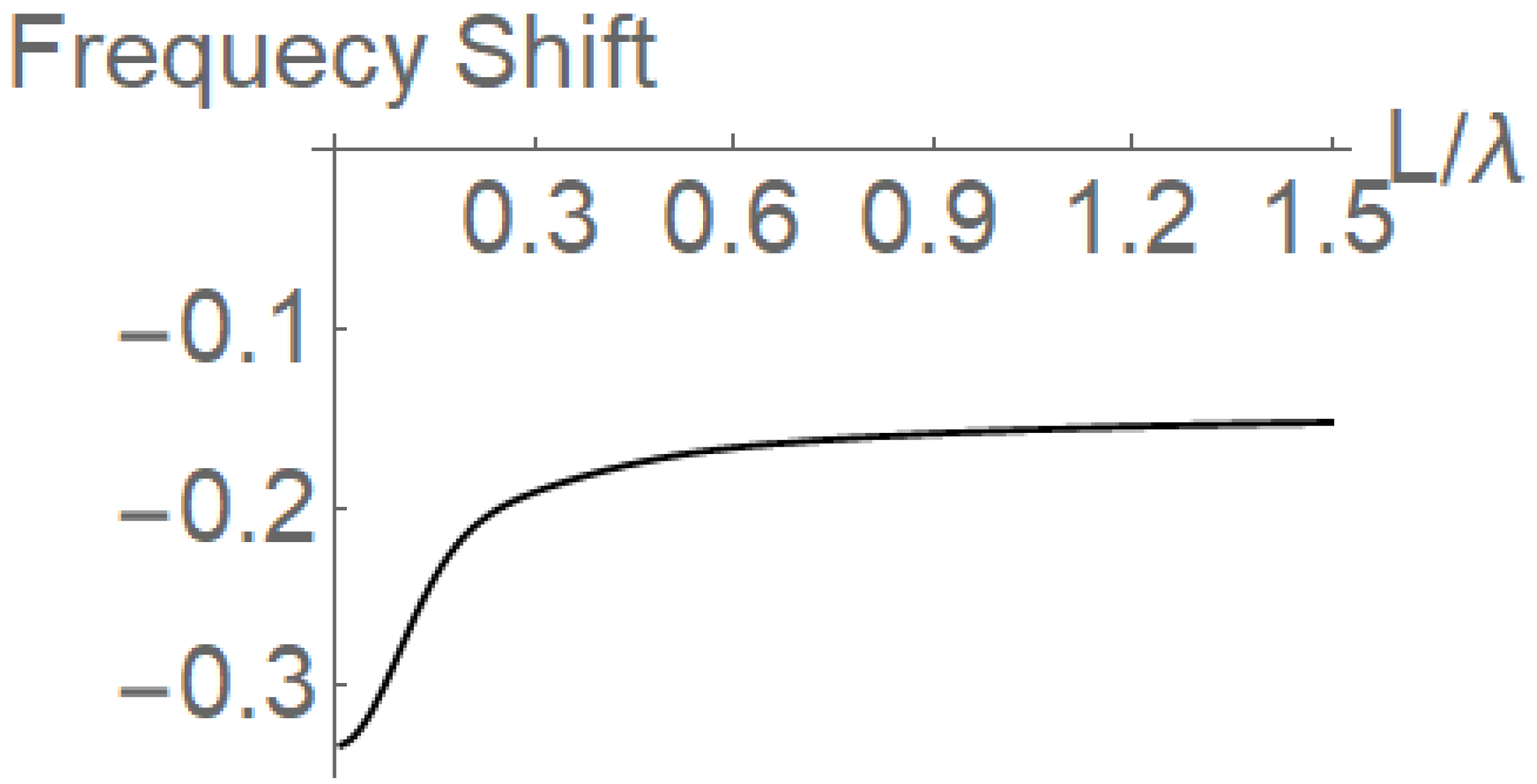
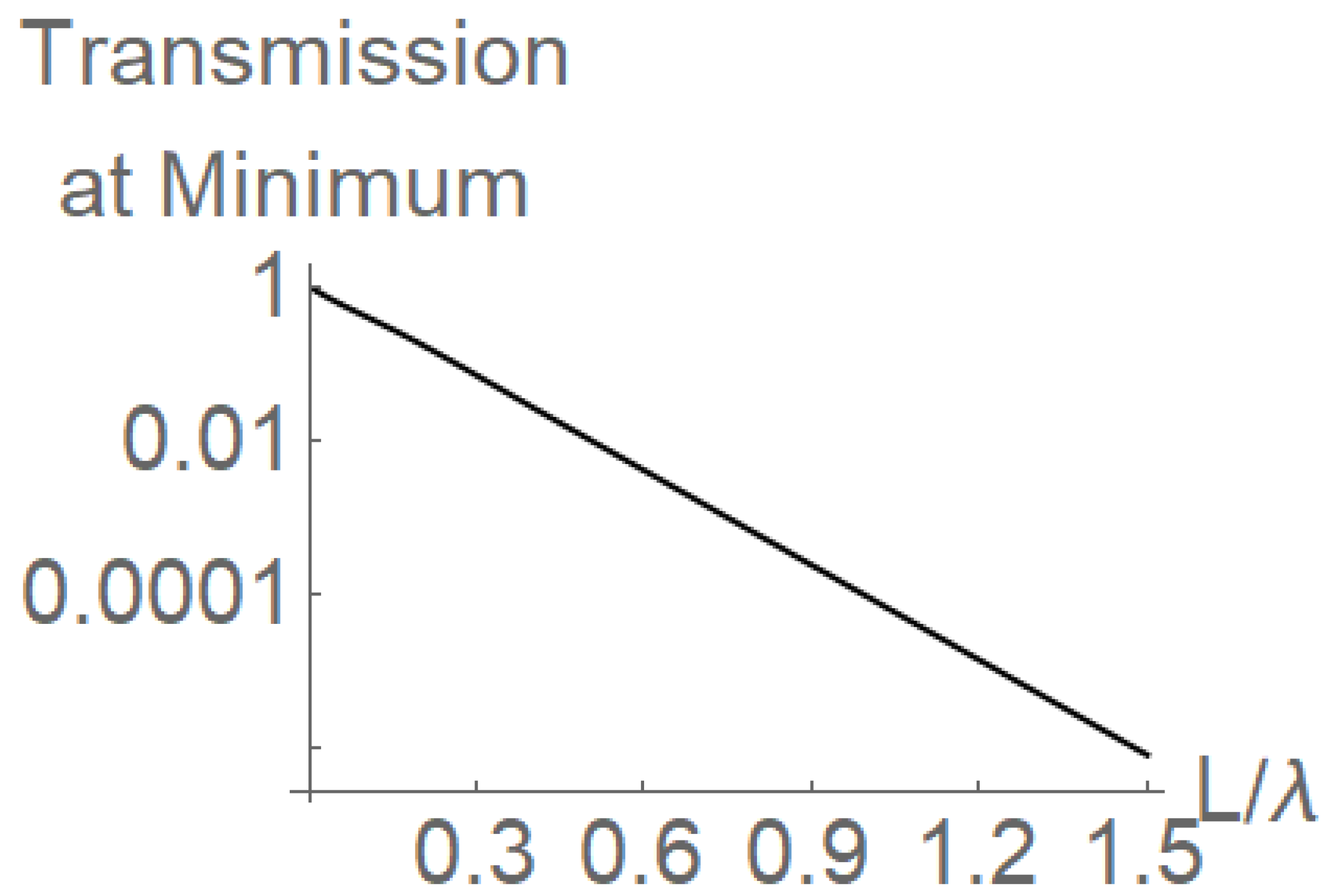
In this section, we summarize the theoretical predictions for the spectrum obtained as a result of the transmission of a cw beam following propagation in a slab configuration when no walls are present. The main qualitative results are:

(a) The magnitude of the frequency shift at the minimum of the transmission curve is a monotonically decreasing function of L (the dimension parallel to the direction of the beam propagation);

(b) The transmission curve as a function of the incident beam frequency is asymmetrical with respect to the line $\Omega ={\Omega }_{shift}$ (${\Omega }_{shift}$ is the value of the normalized frequency at which the transmission curve, for a specific sample length L, has its minimum);

(c) The degree of asymmetry in the transmission coefficient spectrum is dependent on both the length of the sample and the frequency difference, with the most asymmetry near the line center. The thickness L must be many times longer than the resonant wavelength in order for such an asymmetry to be predicted, a condition not satisfied in [3,7,8].

For quantitative predictions, we use the dielectric constant as computed for a pressure-broadened gas, with a $J=0\to J=1$ transition. This is given by the expression [1,2]

$${ϵ}_g(\Omega )=1-\frac{1}{\Omega +0.333+0.5835i}$$

(8)

where $\Omega =\frac{\omega -{\omega }_0}{4\pi n{p}^2/\hslash }$. The quantity $0.333=1/3$ includes only the contribution of the local field correction (Lorentz shift) and not the contribution of the collisional shift (given that the atoms are frozen in a cold-gas experiment), and the quantity 0.5835 is the contribution from the pressure-broadened width as computed in the statistical approximation (valid for frozen atoms).

What one observes in a cw absorption experiment is the ratio of power emerging from the exit face of the slab to the power striking the entrance face. This ratio, the transmission coefficient T, can be obtained from the total transfer matrix

$$M_T(\Omega )=M_{int}({\tilde{n}}_{vac},{\tilde{n}}_{gas})·M_{pp}({\tilde{n}}_{gas},L)·M_{int}({\tilde{n}}_{gas},{\tilde{n}}_{vac}),$$

(9)

where we write $\tilde{n}$ for the index of refraction (as opposed to n = atomic number density). The dielectric constant enters through the relation $\tilde{n}=\sqrt{ϵ}$ for a nonmagnetic medium; in the vacuum we have ${ϵ}_{vac}=1$ and hence ${\tilde{n}}_{vac}=1$.

The object $M_T$ is a (2 × 2) matrix which gives the forward and backward amplitudes in the final region (postexit face) in terms of both forward and backward amplitudes in the initial region (pre-entrance face), in the steady state. It is presented as the product of three (2 × 2) matrices, representing the entrance interface from vacuum to gas, the propagation in the gas from entrance to exit, and the exit interface from gas to vacuum. To obtain from it the transmission coefficient, one observes that there is no backward wave in the postexit region, so that if we represent the initial forward and backward amplitudes by $E_1^{init},E_2^{init}$, we must have

$${\left(M_T\right)}_{22}(E_1^{init},E_2^{init})=0.$$

(10)

This equation can be used to eliminate $E_2^{init}$ so that one is left with a relation between the final forward wave and the initial forward wave. Setting $E_1^{init}=1$, the forward exit amplitude gives the transmission coefficient

$$T=\frac{1}{|\left[M_T(\Omega )\right]{|}_{22}^2}.$$

(11)

This expression is a formal consequence of (9) and (10). To evaluate it, we must examine the three factors of (9). We define the (2 × 2) matrices

$$\mathbf{I}=\left(\begin{array}{cc}1& 0\\ 0& 1\end{array}\right)$$

(12)

$${\sigma }_1=\left(\begin{array}{cc}0& 1\\ 1& 0\end{array}\right)$$

(13)

$${\sigma }_3=\left(\begin{array}{cc}1& 0\\ 0& -1\end{array}\right).$$

(14)

The interface matrix at the entrance face (rightmost factor of (9)) is given by

$$M_{int}\left({\tilde{n}}_{gas}{\tilde{n}}_{vac}\right)=exp((1/2)ln({\tilde{n}}_{gas}/{\tilde{n}}_{vac})({\sigma }_1-\mathbf{I})),$$

(15)

and the one at the exit face (leftmost factor) is

$$M_{int}\left({\tilde{n}}_{vac}{\tilde{n}}_{gas}\right)=exp((1/2)ln({\tilde{n}}_{vac}/{\tilde{n}}_{gas})({\sigma }_1-\mathbf{I})).$$

(16)

The propagation matrix in the gas is

$$M_{pp}({\tilde{n}}_{gas},L)=exp\left(2\pi i{\tilde{n}}_{gas}{\sigma }_3\frac{L}{\lambda }\right)$$

(17)

The following Figure 1, Figure 2 and Figure 3 and Figure 4a,b are based on (11) with (8), (15)–(17). In these figures, the units of frequency are normalized so that the Lorentz shift has a magnitude of 1/3.

5. Cooperative Emission from a Slab without Walls or Collisions

The physical system studied in [9] is to some extent an idealization, in that it is described as a gaseous slab without confining walls; perhaps it can be achieved only in an ultra-cold experiment. Be that as it may, in this ideal system we are able to make extremely accurate (near machine accuracy) calculations, which we call “exact numerical results” (ENR); on the basis of these, we derive important new facts which can be expected to remain at least qualitatively true in achievable systems.

The sample consists of two-level atoms uniformly distributed in a slab with vacuum on both sides. The reason for making it gaseous is that one important finding requires the enlargement of the homogenous transverse line width ${\gamma }_t$ by the introduction of a foreign gas. Apart from this finding, the material could be a solid. If it is gaseous, however, we assume that it is pressure-broadened, i.e., that ${\gamma }_t$ is much greater than the Doppler width, and that the collision shift can be neglected.

The atoms are assumed to begin in the ground state, and are stimulated at time $t=0$ by a very short coherent pulse (duration $<<L/c$) traveling across the slab thickness. To be precise, we take $t=0$ to be the moment after the passage of the pulse, when the atoms (except for a negligibly small region next to the exit face) have not yet felt the reflection from the exit boundary between medium and vacuum. This sets up an initial state in which a fraction of the atoms are excited (we take the pulse to be weak so that this fraction is $<<1$) but the excitation is coherently distributed over all the atoms. The pulse, although short compared to $L/c$, is long compared to $1/{\omega }_0$, where ${\omega }_0$ is the resonance frequency; therefore, it supports a definite frequency which we set to be ${\omega }_0$.

We denote by $\overrightarrow{E}$ the Maxwell electric field, which we take as complex with a dominant $exp(-i\omega t)$ oscillation, and by $\overrightarrow{P}$ the polarization density which we regard as a continuous function of space and time. Actually, we assume that the only spatial dependence in the problem is on z, which measures movement from the entrance face. Thus, we take $\overrightarrow{P}$ as proportional to the quantum mechanical amplitude $b(z,t)$ for the excited state, which is the same for all atoms of a given $z,t$.

We detach the electrodynamics from the physical properties of the matter by starting with a one-dimensional integral operator, derived purely from Maxwell’s equations, that gives the field at one point due to the polarization at another, and introducing a single constant for the response of the polarization to the field. Thus, the field can be eliminated, and in the weak-pulse problem one is left with a linear equation giving the time rate of change of the polarization in terms of itself, after the passage of the exciting pulse.

We use an integral operator rather than the second-order differential form of Maxwell’s equations. The kernel $G(z,z^{\prime })=exp(i{k}_0|z-z^{\prime }\left|\right)$ (see Equation (19) below) contains the effect of both backward and forward waves, so that the neglect of the backward wave [11] is avoided. The price is that in the eigenfunctions of this operator, the wave number $k_0$ is replaced by a complex wave number $k^{\prime }$ so that the operator is not hermitian. Consequently orthogonality of two eigenfunctions is of the form $\int {\varphi }_1\left(z\right){\varphi }_2\left(z\right)dz=0$ rather than $\int {\varphi }_1\left(z\right){\varphi }_2{\left(z\right)}^{*}dz=0$.

The spatial direction of $\overrightarrow{E}$ is an unchanging direction in the lateral plane of the slab. Therefore, we write the field as a scalar E, but before entering the medium it oscillates as $exp(-i{\omega }_{0}t)$.The fundamental equations for the system are

$$\dot{b}(z,t)-i{\omega }_{L}b(z,t)+{\gamma }_{1}b(z,t)=3i{\omega }_{L}E(z,t),$$

(18)

where

$$E(z,t)=-i(k_0/2){\int }_{-z_0}^{z_0}exp(i{k}_0|z-z^{\prime }\left|\right)b(z^{\prime },t).$$

(19)

The quantity ${\omega }_L$ is taken in [9] to be positive; the actual Lorentz shift is $-{\omega }_L$. Furthermore, all frequencies in [9] are written in units of $4S$ (see Section 1) so that the magnitude of the Lorentz shift is $1/3=0.333$.

Note that E arises entirely from the polarization density, since the original pulse has already left through the exit face at the time $t=0$. Reflection from that face is included in b.

After eliminating E from (18) and (19), one gets a linear integrodifferential equation for b, whose eigenfunctions satisfy (writing $z_0$ for $L/2$)

$$\mu \varphi \left(z\right)=3{\omega }_L(k_0/2){\int }_{-z_0}^{z_0}G(z,z^{\prime })\varphi \left(z^{\prime }\right)d{z}^{\prime },$$

(20)

which has eigenfunctions of the form $\varphi \left(z\right)=a_{f}exp\left(i{k}^{\prime }z\right)+a_{b}exp(-i{k}^{\prime }z)$. The eigenfunctions turn out to be either odd or even in z, thus:

$$\begin{array}{c}\hfill {\varphi }_s^o\left(z\right)=sin\left({\left(k^{\prime }\right)}_s^{o}z\right)\\ \hfill {\varphi }_s^e\left(z\right)=cos\left({\left(k^{\prime }\right)}_s^{e}z\right)\end{array}$$

(21)

where the subscript s enumerates the modes of each type.

After some reasoning, we arrive at transcendental equations determining the complex wave numbers ${\left(k^{\prime }\right)}_s^o,{\left(k^{\prime }\right)}_s^o$ and the complex eigenvalues ${\mu }_s^o,{\mu }_s^e$. These equations are readily solved by computer; the computer-intensive task is to obtain quantities of physical interest by summing over a large number of modes. Empirically, we determined how many modes were necessary in a particular case by exploring whether the inclusion of additional modes changed the answer. The results of such summations constituted our “exact numerical results” (ENR). In certain cases, we were able to duplicate such a result by some other method that is completely independent of ENR, and the agreement to several decimals confirmed the validity of both methods.

A number of new results are described in [9], but we shall cite only a single one for our present purpose. The field strength emanating from the forward (exit) face at time ts was found by ENR to be

$$E_f\left(t\right)=Aexp\left([-({\gamma }_t-i{\omega }_L)t]\right){\mathrm{\Sigma }}_s[-{\left(c_s^o\right)}^2{N}_s^{o}exp(-{\mu }_s^{o}t)+{\left(c_s^e\right)}^2{N}_s^{e}exp(-{\mu }_s^{e}t)].$$

(22)

where $c_s,N_s$ are explicit functions of the complex wave vector $k_s^{\prime }$ for mode s.

This is easily integrated term by term to give the spectral amplitude as

$$f\left(\omega \right)={\int }_0^{\infty }{E}_f\left(t\right)exp\left(i\omega t\right)dt=A{\mathrm{\Sigma }}_s[-\frac{{\left(c_s^o\right)}^2{N}_s^o}{{\mu }_s^o+i\Omega +{\gamma }_t-{\omega }_L}+\frac{{\left(c_s^e\right)}^2{N}_s^e}{{\mu }_s^e+i\Omega +{\gamma }_t-{\omega }_L}],$$

(23)

where $\Omega =\omega -{\omega }_0$.

We then defined a “center-of mass” frequency shift as

$$\tilde{\Omega }=\frac{{\int }_{\infty }^{\infty }{\left|f(\Omega )\right|}^2\Omega d\Omega }{{\int }_{\infty }^{\infty }{\left|f(\Omega )\right|}^{2}d\Omega }.$$

(24)

(The prefactor A in (23) cancels out here).

The integrals in (24) can be calculated analytically term by term, but each term involves a pair of modes; this operation is therefore the most computer-intensive of the ENR calculations. The numerator appears to be a logarithmically divergent integral, but it really is finite since the contributions from ∞ and $-\infty$ cancel asymptotically.

Comparing the ENR calculation of (24) at various thicknesses with the Formula (6), we found poor agreement. This is not surprising, inasmuch as (6) applies only to the initial radiation spectrum, while the ENR takes into account the time development. In particular the decay of the atomic excitation through the term ${\gamma }_1$ in (18) is not allowed for in (6). The disparity between (6) and (24) is exhibited in

Table 1. ENR frequency shifts vs. FHM [1] prediction.

Thickness $\mathit{L}/\mathit{\lambda }$	ENR	FHM
0.00	–0.333333	–0.333333
0.05	–0.317258	–0.317206
0.10	–0.273891	–0.272540
0.15	–0.217005	–0.209471
0.20	–0.162915	-0.141801
0.25	–0.122385	–0.083333
0.30	–0.098172	–0.044355
0.35	–0.087639	–0.029274
0.40	–0.086172	–0.036031
0.45	–0.089305	–0.057348
0.50	0.093580	–0.083333
0.55	–0.096778	–0.104594
0.60	–0.097874	–0.114868
0.65	–0.096862	–0.112442
0.70	–0.094436	–0.100038
0.75	–0.091577	–0.083333
0.80	–0.089151	–0.068716
0.85	–0.087654	–0.061074
0.90	–0.087152	–0.062310
0.95	–0.087383	–0.071024
1.00	–0.087931	–0.083333
1.05	–0.088402	–0.094470
1.10	–0.088542	–0.100534
1.15	–0.088281	–0.099786
1.20	–0.087712	–0.093078
1.25	–0.087020	–0.083333
1.30	–0.086400	–0.074338
1.35	–0.085982	–0.069318
1.40	–0.085807	0.069819
1.45	–0.085833	–0.075269
1.50	–0.085963	–0.083333

. The ENR results damp out the strong oscillations predicted by (6), for thickness L from $0.2$ to $1.4\lambda$.

This suggests that if the transverse broadening ${\gamma }_t$ were made much larger than ${\gamma }_1$, the power spectrum would be dominated by the radiation at small t and the ENR would show closer agreement with (6). Accordingly, we tried increasing ${\gamma }_t$ to $72{\omega }_{\left|LL\right|}$ (with ${\omega }_{\left|LL\right|}=1/3$, this is 41.25 times the value 0.5835 given in (8)). The result, shown in Figure 7 of [9], is spectacular. The ENR frequency shift tracks Formula (6) almost precisely as a function of L, through several well-defined oscillations from $L=0$ to $L=1.5\lambda$. The period $\delta L=\lambda /2$ is unmistakable.

The dependence of the ENR shift on the enhancement ratio ${\gamma }_t\left(enhanced\right)/{\gamma }_t\left(unenhanced\right)$ is shown in

Table 2. ENR shifts at $L=0.35\lambda$ with variable enhancement.

Enhancement Ratio	ENR Shift with Enhancement
1.0	0.087639
1.2	0.082708
1.4	0.078563
1.6	0.075023
1.8	0.071962
2.0	0.069286
3.0	0.059738
5.0	0.049887
6.0	0.047016
7.0	0.044845
8.0	0.043147
9.0	0.041783
10.0	0.040664
12.0	0.038933
14.0	0.037659
16.0	0.036681
18.0	0.035908
20.0	0.035281
22.0	0.034762
24.0	0.034326
26.0	0.033954
28.0	0.033633
30.0	0.033353
32.0	0.033107
34.0	0.032889
36.0	0.032694
38.0	0.032519
40.0	0.032361
42.0	0.032218
44.0	0.032088
46.0	0.031968
48.0	0.031859
50.0	0.031758
52.0	0.031664
54.0	0.031578
56.0	0.031497
58.0	0.031422
60.0	0.031351

for constant $L=0.35\lambda$, the thickness at which Table 1 shows the maximum disparity between (6) and (24). The enhancement ratio of 40 gives a shift of $-0.032361$, very near to the shift of $-0.029274$ predicted by (6). An enhancement ratio of 10 gives $0.040664$, which is not too bad, but any lesser enhancement is clearly insufficient.

We are aware that to produce this effect in a real pulse-excited system by the introduction of a foreign gas to enhance the line broadening would be a difficult challenge. However, if it could be done, the experimenters would be entitled to say, after subtracting the known Lorentz shift, that they had made a genuine measurement of the cooperative Lamb shift in a slab as originally defined [1].