Abstract
We generalize Schrödinger’s factorization method for Hydrogen from the conventional separation into angular and radial coordinates to a Cartesian-based factorization. Unique to this approach is the fact that the Hamiltonian is represented as a sum over factorizations in terms of coupled operators that depend on the coordinates and momenta in each Cartesian direction. We determine the eigenstates and energies, the wavefunctions in both coordinate and momentum space, and we also illustrate how this technique can be employed to develop the conventional confluent hypergeometric equation approach. The methodology developed here could potentially be employed for other Hamiltonians that can be represented as the sum over coupled Schrödinger factorizations.
1. Introduction
The Hydrogen atom was originally solved by Pauli employing operator methods by discovering the Lie algebra of the SO(4) symmetry in the problem [1]. Schrödinger followed shortly with the differential equation approach of wave mechanics [2,3]. In 1940, Schrödinger developed the factorization method for quantum mechanics [4] and employed it to solve Hydrogen as well [5]. This factorization method was extensively reviewed by Infeld and Hull [6]. Our focus in this work is on an operator-based method to solve Hydrogen. Similar to how the wave-equation approach can be solved directly in Cartesian coordinates [7], we develop here the Cartesian factorization method for Hydrogen. While it shares some of the characteristics of the spherical coordinate-based factorization method, it is distinctly different. It is surprising that one can discover a new methodology for solving Hydrogen nearly one hundred years since its first solution.
There are two new developments that arise with this solution. First, this approach generalizes the Schrödinger factorization method, which employs a single raising and lowering operator factorization, into an approach that works with the sum over three coupled raising and lowering operator factorizations—one for each Cartesian coordinate. These raising and lowering operators also depend on the radial coordinate, so the operators corresponding to the different Cartesian directions do not commute with each other. Nevertheless, a full operator-based approach can be employed to solve the quantum problem. Second, the strategy used here, where we solve first for the energy eigenstate as a sequence of operators acting on the ground state of an auxiliary Hamiltonian, allows us to then construct the eigenfunctions in both real space and momentum space by simply projecting onto the coordinate-space and momentum-space eigenfunctions, whereby both solutions proceed using the same methodology. This is quite different from conventional differential equation approaches, which are quite dissimilar for coordinate and momentum space. It does turn out that the algebra required for the momentum-space eigenfunctions is somewhat more complicated than for the real-space functions.
Conventional quantum mechanics suffers from overuse of the coordinate-space representation. This is solely for convenience—the Schrödinger equation is a second-order linear differential equation in coordinate space; in momentum space, it generically becomes an integral equation, which is much more difficult to work with. One might argue that this is just fine. After all, the Stone–von Neumann theorem [8,9] tells us that all representations are equivalent to the coordinate-space representation. However, the ability to formulate quantum mechanics in a representation-independent fashion is an important cornerstone of the theory. In this work, we show how to determine wavefunctions independent of the basis.
One other notable result is that nearly all of the operator-based derivations we employ can be performed without using any calculus. We illustrate this throughout the paper. Calculus ends up being needed only for the normalization of the wavefunctions and for the derivation of some identities we require when calculating the momentum-space wavefunctions. Of course, one can map this problem onto a differential equation as well. We illustrate how one can extract the conventional confluent hypergeometric equation for the wavefunction of Hydrogen in coordinate space below.
While the differential equation approach to solving Hydrogen in spherical coordinates is performed in almost every quantum textbook, the operator method in spherical coordinates is limited to only a handful of textbooks. Starting with Harris and Loeb [10], and followed shortly thereafter by Green [11], Bohm [12], Ohanian [13] and de Lange and Raab [14], Schrödinger’s factorization method (and the closely related ladder-operator method) has been covered amply in many texts. One might even say it has been increasing in popularity, as it has appeared in a number of recent texts as well, including Hecht [15], Binney and Skinner [16], Schwabl [17] and Razavy [18]. All of these texts employ essentially the same technique, closely related to Schrödinger’s original method [5]. Only de Lange and Raab [14] also solve the problem in momentum space, but they employ a direct operator problem formulated in momentum space, which is a completely different technique and is not closely related to the coordinate-space approach. Judd [19] also solves the problem directly in momentum space by determining the spherical harmonics of a four-sphere, following Fock’s original derivation [20].
Here, we proceed differently. The Cartesian factorization of the Coulomb Hamiltonian was first worked out by Andrianov, Borisov and Ioffe in 1984 [21]. We begin by writing down the Hydrogen Hamiltonian as
where we use hats to denote operators, ( y, and z) are the momentum operators in the th direction, are the corresponding coordinate operators, and , with ℏ Planck’s constant. We work in electrostatic units, where is the magnitude of the charge of a proton or electron, m is the mass of the electron, and . Reduced mass effects are taken into account by simply replacing , but all of our formulas here will use m for the mass.
The Cartesian factorization rewrites the Hydrogen Hamiltonian in the following form:
where the raising and lowering operators are Hermitian conjugates given by
Here, we have used , which is the Bohr radius, and that the energy satisfies
In the Hydrogen Hamiltonian, we have , but we will be using these operators and energies for different values of throughout the work.
The verification that Equation (2) is equal to Equation (1) follows from a direct computation. We have
We use the fact that , which can be employed to show that (for further details, see the appendix in [22] and Section 2 below). The commutator can then be computed, and yields
Summing over the spatial indices immediately gives us
Hence, we find that Equations (2) and (4) produce the Hydrogen Hamiltonian and ground state energy when we set .
Note that the raising and lowering operators do not commute with each other for different Cartesian coordinates. Hence, the factorization involves coupled operators and is different in character from the Cartesian factorization of the isotropic simple harmonic oscillator in three dimensions, where the raising and lowering operators for different directions commute with each other.
The form of the Hamiltonian in Equation (2) allows us to directly determine the ground-state energy and the ground-state wavefunction in coordinate space. Because the factorized form of the Hamiltonian is the sum of positive semidefinite operator terms and a constant, the ground-state energy is given by the constant and the ground-state wavefunction satisfies
for all . We use the symbol to denote the ground state of the auxiliary Hamiltonian
which satisfies
for fixed (and all ) with energy .
We find the ground-state wavefunction by taking the overlap of Equation (8) with the position eigenstate bra :
Using the condition for the ground-state wavefunction in Equation (8), we find that
We can proceed in one of two ways at this point. We can use the coordinate-space representation of the momentum operator, given by , to find the three differential equations
These three equations can be immediately solved via
This is the well-known ground-state solution for Hydrogen, with the overall normalization constant still needing to be determined.
We can also solve this problem without calculus. However, it turns out the algebra for this is a bit more complex. We illustrate why here and provide some additional details in the Appendix A. First, we use the translation operator to write
Then, we compute
To evaluate this expression, we want to use Equation (8) to replace by . There are two issues that arise for this: (i) one cannot immediately evaluate operators such as onto the coordinate eigenstate at the origin, without some appropriate limiting procedure and (ii) the fact that does not commute with creates many additional terms that one must carefully keep track of. It is easier to discuss a strategy for how to work on this after one has developed a bit more formalism, so this discussion continues in the Appendix A. The full expression of the translation operator and the methodology needed to complete the algebraic determination of the maximal angular momentum wavefunctions has already been completed elsewhere [22].
The momentum wavefunction is also not so simple to determine and we postpone discussing it until we work on the general case below. The organization of the remainder of the paper is as follows: in Section 2, we derive the operator form for the eigenfunctions and eigenvalues for the general case after briefly summarizing the properties of harmonic polynomials. The coordinate-space wavefunctions are derived in Section 3 and the momentum space wavefunctions in Section 4. Section 5 provides a derivation of the more conventional confluent hypergeometric equation approach. We conclude in Section 6.
2. Deriving the Energy Eigenstate
We begin with a short “tutorial” on how to compute commutators without taking derivatives or working with an explicit representation for the operators. This methodology was introduced by Dirac [23], and is an elegant way to determine commutators without calculus. A rather complete discussion can also be found in the appendix in [22]. We employ this methodology throughout.
To begin, we note that the commutator of with , is simple to compute, but by also employing the product rule, we quickly learn that
or . Note that we have to move the commutator through to complete this derivation. This is easy to establish a posteriori, but it can actually be directly verified by the Jacobi identity and the fact that the operator has the same eigenvectors as the operator [12,22]. With a simple inductive argument, one can then establish that , for all integers n.
Next, we work with the Hermitian (but not self-adjoint) radial momentum operator, , defined to be
One immediately sees that
after using the identity derived above and the fact that . The radial momentum determines the radial component of the kinetic energy , separating it into the radial component and the perpendicular component via
The perpendicular component of the kinetic energy commutes with the radial coordinate, as can be seen by direct computation:
The cancellation follows from a simple rearrangement of operators using the commutation relation and the definition of the radial momentum in Equation (18).
One of the subtleties we have to work with is that the Cartesian components of momentum do not commute with the radial momentum. In particular, we find that
Similarly, the Cartesian components of position do not commute with the radial momentum
These results allow us to compute our final commutator, that of the radial momentum with the perpendicular kinetic energy:
which follows after some complex algebra.
We do not use a separation of variables into radial and angular coordinates, nevertheless, similar to the Cartesian differential equation approach [7], we need to work with harmonic polynomials, but here in operator form. Kramers originated the use of harmonic polynomials for angular momentum [24] (see also Brinkman [25] and Powell and Crasemann [26]), which has been revitalized recently by Weinberg [27]. Here, we follow the approach of Avery [28] and define the lth-order harmonic polynomial to be a homogeneous polynomial, so that
for l a nonnegative integer. Here, we have . Note that the radial momentum operator is a Hermitian operator that is conjugate to the radial coordinate operator and satisfies Equation (19).
The result in Equation (25) follows by simply evaluating the commutator, which yields a term given by times the monomial term for every coordinate factor in each monomial term of the polynomial; when the polynomial is homogeneous, the number of terms in each monomial is the same, and hence, the entire polynomial is multiplied by . In addition, these polynomials satisfy Laplace’s equation, written in the operator form
These harmonic polynomials are defined up to an overall multiplicative factor. The low-order ones are just what we expect them to be from our knowledge of Cartesian spherical harmonics. The zeroth-order one is just 1. The first-order ones are , , and . The second-order ones are , , , , and . One should note that the harmonic polynomials have all the dependence removed from them, because the Laplacian of is nonzero. We will be employing the harmonic polynomial operators heavily in the derivation below.
However, before getting there, we want to note one other special property about the harmonic polynomials. First, we can easily verify from the commutation relations derived above that
which then implies that
The factor is needed to divide each of the l factors in each monomial term of the harmonic polynomial to ensure that each monomial commutes with the radial momentum.
Now, with these technical details finished, we are ready to move on to the derivation of the eigenfunctions and eigenvalues of Hydrogen. In Schrödinger’s original factorization method, he constructed higher-energy states by acting a chain of operators on the ground state of an auxiliary Hamiltonian, which was related to the original Hamiltonian, but employed a series of different raising and lowering operators, as well as different constant terms. He derived this result by showing that the wavefunction constructed must be an eigenfunction of the original Hamiltonian. We will follow similar strategy here, but it has a few places where the steps are modified because our Hamiltonian has a sum of factorized terms instead of just one. While it may seem like we are just going to guess the solution and then verify it, which is a valid approach, the motivation for the guess comes from the standard operator formalism solution for Hydrogen.
To begin, we first must define another set of raising and lowering operators that we call and , with . The operator is defined by
following de Lange and Raab’s convention [14]. This operator can be expressed in terms of our Cartesian operators as follows:
One can immediately verify that
Before we construct the ansatz for the eigenstate, we need to establish the following identity:
The proof requires a number of steps. First, we establish the action of the radial momentum on the auxiliary Hamiltonian ground state via
where we used the fact that implies that
for all . Second, we show that .
This is done with the following steps:
where Equation (33) is applied twice. Next, we evaluate acting on the harmonic polynomial and the auxiliary Hamiltonian ground-state via
because . We evaluate each piece of the commutator next. First, we compute
In the second line, the double commutator vanishes because the harmonic polynomial satisfies Laplace’s equation as shown in Equation (26), while the second term simplifies because the harmonic polynomial is homogeneous, as shown in Equation (25). We used the definition of the Bohr radius to simplify the final result as well.
The second piece of the commutator is
We also need to determine how commutes with . A direct computation, employing Equations (21) and (24) yields
This equation can be rearranged to an intertwining relation
indicating that the operator can be moved through by shifting the latter operator to . One can derive a similar intertwining relation given by
In the Schrödinger factorization method, an intertwining relation is employed to construct the higher-energy eigenstates of the original Hamiltonian from a series of raising operators acting on an auxiliary Hamiltonian ground state. Here, we employ the exact same technique, except the intertwining relation is complicated due to the fact that it generates many extra terms proportional to . Since these terms vanish when they operate on , they do not corrupt the final intertwining relation, but they make the derivation more cumbersome. We now go carefully through the construction of all of the remaining eigenstates.
We start with the modification of the intertwining relation, which is derived by commuting through :
This derivation proceeds by first using the top relation in Equation (31). Next, we construct the Hamiltonian via the lower relation in Equation (31) and also employ the commutator in Equation (39). This differs from the conventional intertwining relation due to the extra term on the last line of Equation (42).
We now show how to determine the energy eigenstates using a quasi-inductive argument. We build up subsequent eigenstates and see why, in each case, the values used are integers chosen according to a specific procedure. This ends up being a constructive methodology for generating the energy eigenstates.
We begin with an ansatz for the first (unnormalized) eigenstate in the chain of eigenstates. It has the form (with the subscript of to be understood a posteriori)
Here, the symbol in the ket on the right-hand side is a parameter, and our initial goal is to show that we must have and . To do so, we act onto this state, which yields
Our first step is to move through the powers of . This is possible because , as we now show
Verifying this result required us to use three facts: ; and the definition of the radial momentum in Equation (18).
This commutator means we can move the operator through the power of and have it act on the harmonic polynomial operator and the state. We use the identity in Equation (32) to replace the term by a number, yielding
What remains to do is operating onto the state. We need Equation (33) for the action of the radial momentum onto the auxiliary Hamiltonian ground state and the fact that we can commute through . This leaves us with the final calculation
Substituting into Equation (46) and using the definition of the Bohr radius gives us
Clearly, we must have and (which means , because we also require ) in order for this to be an eigenstate, with the eigenvalue given on the last line. This establishes the correct integers for the first eigenstate in the series. The requirement that arises when we construct the ground-state wavefunction (see Appendix A)—if we do not make this requirement, then the ground-state wavefunction is not normalizable. We apply this constraint here, knowing this requirement.
For the general case, we choose a set of real and nonnegative parameters and form the trial eigenstate via
When we act from the left, we can move it through the terms one by one to the right. It will generate a number of terms proportional to , for some number C, but those will all vanish when operated to the right against the state, because we will organize the terms so that . We are then left with
Acting to the right proceeds exactly like what we did above and yields
Clearly, we must have again that . To determine the terms, we must determine the factor C when moves to the right past , for each value of k such that . A simple calculation shows that
Starting from the first term, we must have , otherwise . Given , then we have must satisfy , or (because all are nonnegative). Continuing, in turn, we immediately see that we must have for the state to be an eigenstate. Then, we have
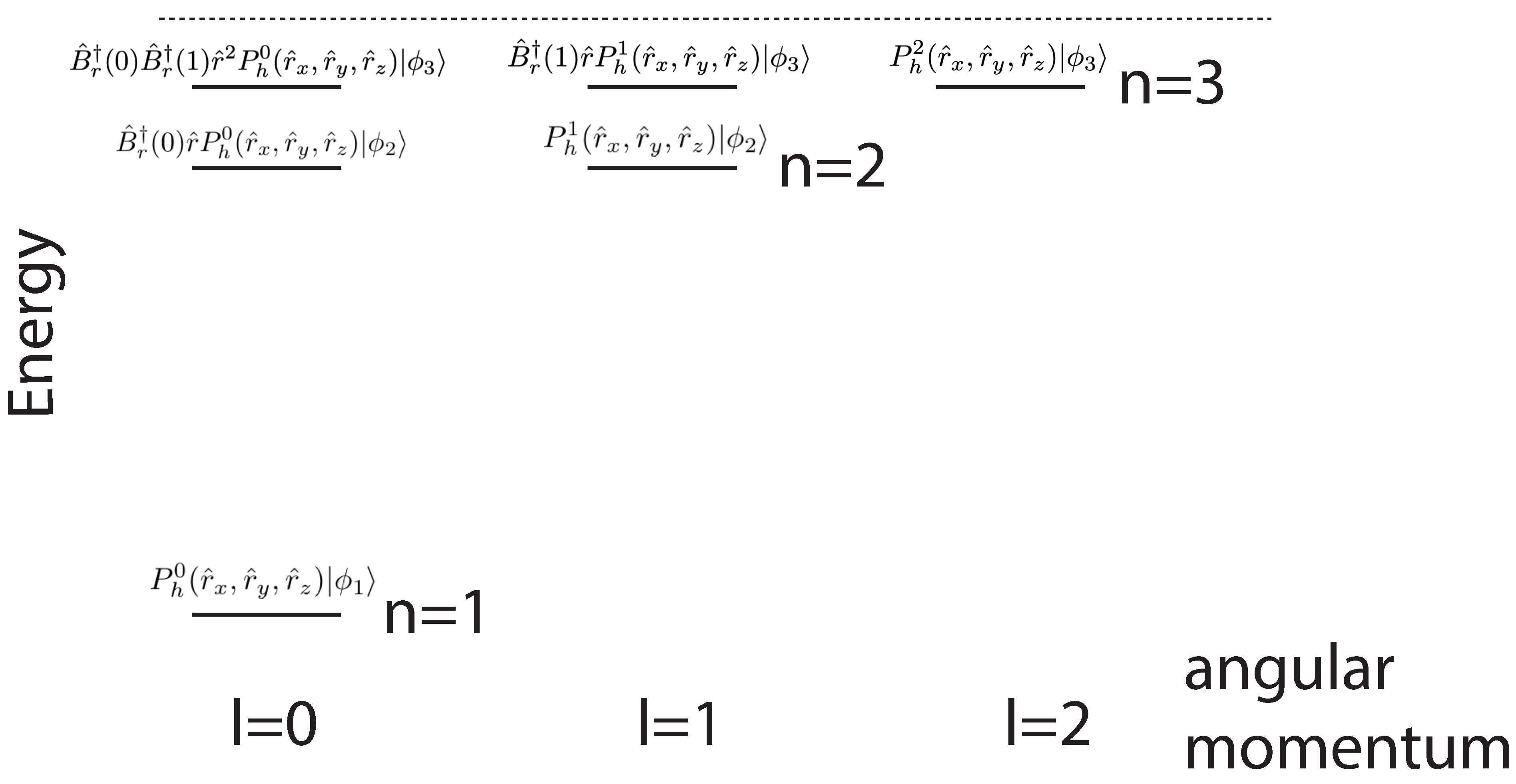
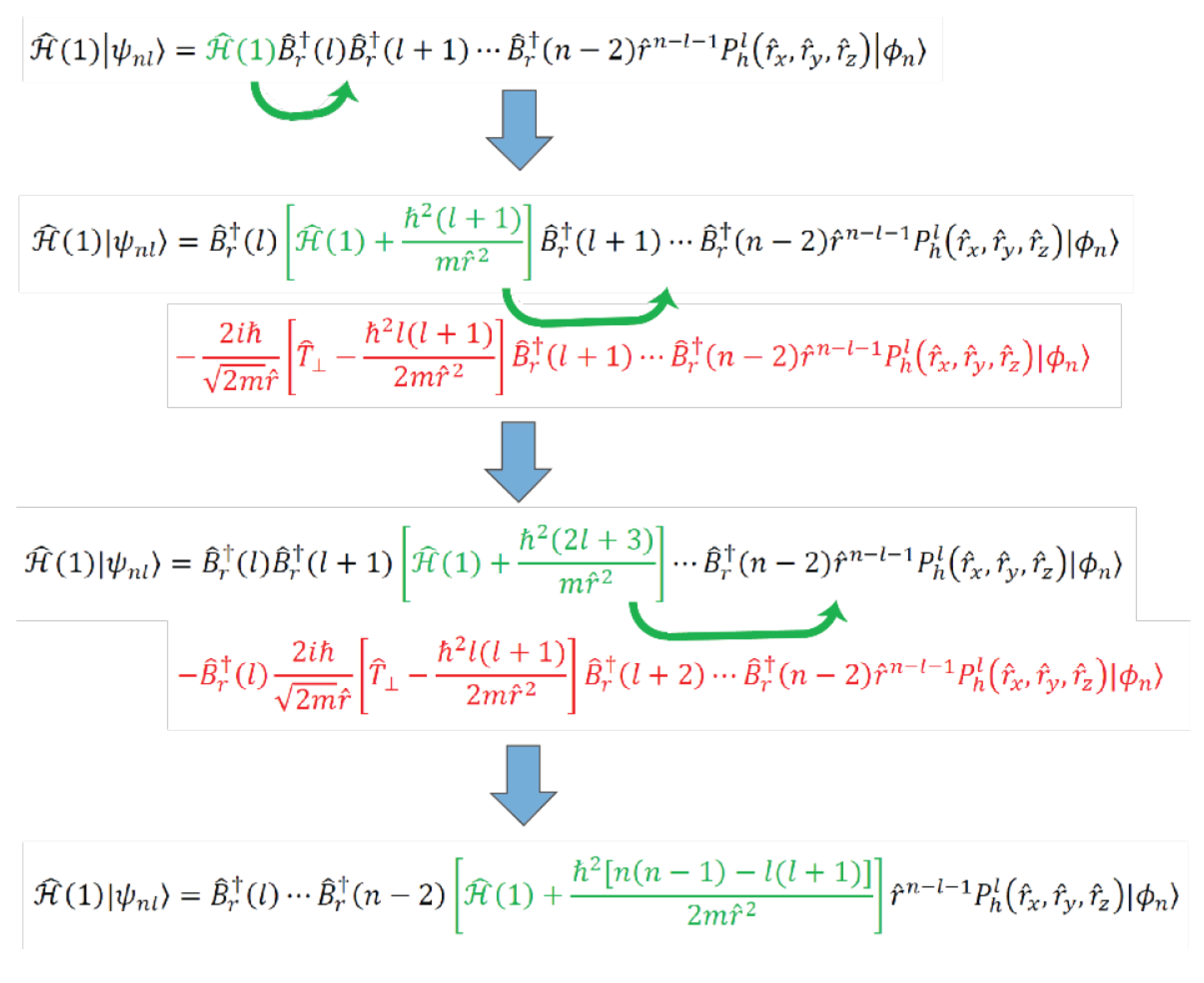
which further tells us that we must have again. Hence, and the energy eigenvalue is —the same value for every state in the chain that we can create, down to . This completes the argument that we must choose consecutive integers in the chain of operators to yield an energy eigenstate. The results are shown in Figure 1 for the first three energy multiplets. We next establish these results rigorously, deriving all of the required details. A schematic of how the calculation is structured is given in Figure 2.
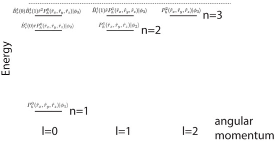
Figure 1.
First three energy eigenstate multiplets, plotted to show the energy and the corresponding state, along with the angular momentum. The energies are the same for all inequivalent harmonic polynomials with the same l value. The dotted line is the limit point for the energy eigenvalues.
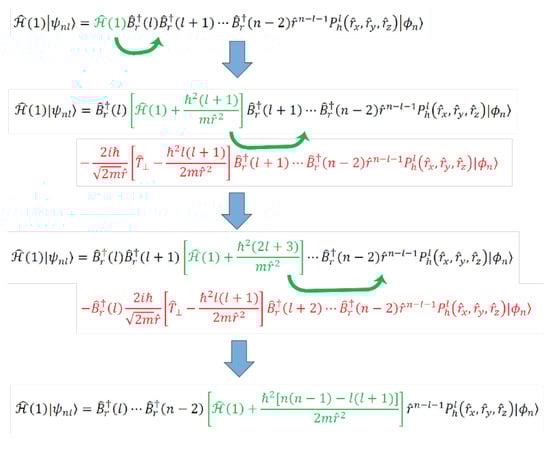
Figure 2.
Schematic for how the energy eigenstate calculation works.
We next establish the following identity, which involves multiple applications of the intertwining identity to move the Hamiltonian operator through the sequence of raising operators involving the product with chosen from the factors in order from left to right:
We proceed by induction. One can immediately verify that if we set , then Equation (42) is the base case for the above intertwining identity. We next assume it holds for the above case and proceed to show it also holds when we add the operator to the product on the left. This yields
after using Equation (42). Now, we employ Equation (54) along with (40) and (41) to find
The terms in the last two rows can be combined with those in the upper rows to finally yield
This completes the inductive proof.
When constructing an ansatz for the eigenfunctions, we will find that the fact that the operators have integer parameters will require the power of and the parameter to both be integers. So, we choose and the integer degree of the harmonic polynomial l to label the eigenstate via
with the restriction that because harmonic polynomials are not defined for negative l, and our wavefunction ansatz restricts l to be less than n. Now, we verify that it is indeed an eigenfunction and we also determine the eigenvalue.
This is the homestretch, but it still takes a number of steps. We use the intertwining relation (recalling all of the extra terms vanish when acting on the state to the right) and find that
which follows from Equation (54) and because the sum satisfies
Next, we recall that and focus on evaluating the term from the total kinetic energy as follows:
For the last term in Equation (61), we have
The first term in Equation (61) is evaluated by directly computing the commutator, which uses a number of the operator relations we already derived above (including the commutator in Equation (28), the identity in Equation (32), and the action of on in Equation (33)). The result becomes
Note that it is at this point where we require . If this was not the case, the term proportional to in the last equality would have a coefficient of instead of . We only obtain an eigenstate if the coefficient is exactly . Combining all of these results then gives
Introducing this result into Equation (59) finally shows that
which is the eigenvalue-eigenvector relation we wanted to establish.
We have not yet considered the normalization of the wavefunction. To do this, we must compute the norm
We replace in the center and then commute the terms through. Using the results we have derived in computing the eigenfunction above, a careful calculation shows that this result is equal to the factor multiplied by the expression in Equation (66) with the middle two factors removed. Continuing in this fashion, we find that
We assume that the initial state is normalized and we choose the harmonic polynomials to be normalized when integrated over the angular variables only. In other words, we choose the harmonic polynomials, which can be multiplied by an overall constant, in such a fashion that
Since is a linear combination of the conventional spherical harmonics, the above relation simply says the angular part of the wavefunction is normalized (given that the radial part was already normalized). This is because it can be converted into an integration over the angular parts of the squared wavefunction (a discussion for how to do this in general is given in the work on the spherical translation operator [22]). Or one can directly evaluate the matrix element, and scale the harmonic polynomial to force it to be equal to 1. Then, we find that the normalized eigenstates are
with the normalization factor for the auxiliary Hamiltonian ground state satisfying
The last result requires calculus to compute, and is the standard normalization condition. Note that the e appearing in the denominator of Equation (69) is the electric charge of the proton.
This derivation has produced all of the bound states of Hydrogen labeled by the principle quantum number n and the total angular momentum l. However, because we are working with harmonic polynomials, we are not generically in an eigenstate of the z-component of angular momentum. We have the restriction that , which implies that there is a degeneracy across l and we have determined the well-known bound-state energy . All of this is as expected, but it used no angular momentum and no calculus (except for the final normalization step)!
3. The Wavefunction in Coordinate Space
Now, we focus on determining the coordinate representation for the unnormalized wavefunction given by the overlap
This wavefunction can also be found algebraically, employing no calculus, as we show next.
To begin, we first determine , which satisfies
We can immediately act the harmonic polynomial on the coordinate state to the left to obtain
Then, we use the techniques from Equations (15), (16) and the Appendix A to find the result generalizing Equation (14) as follows:
where is the normalization constant in Equation (70). This requires calculus to determine it in the usual fashion. Note that this result might not be in a form that is easily recognized, since we do not have a conventional spherical harmonic factor. Rest assured, this result is the same as the conventional result, with a radial wavefunction behaving like near the origin. We simply rewrite it as
where the last term is a properly normalized linear combination of the conventional spherical harmonics ; that normalization is with respect to the angular coordinates.
For the general wavefunction , we must work with the operators. The general wavefunction satisfies
The first step is to note that we can move the “spherical harmonic” factor all the way to the left and have it act on the position eigenstate because that term commutes with all operators. Doing so gives
and we focus all of our efforts on evaluating the remaining matrix element. Note that evaluating a generic term, such as can always be carried out by using Equation (33) and the relation
So, each time a operator acts on a power of multiplied by an auxiliary Hamiltonian ground state, it produces a number times the same power plus another number times the power minus one. Hence, the remaining matrix element in Equation (77) is a polynomial in r of degree (that has a lowest power of ) and is multiplied by the auxiliary Hamiltonian ground-state wavefunction (exponential function) in Equation (75).
We call this (unnormalized) radial wavefunction , which satisfies
The factor is just a phase factor, which is introduced so that this function agrees with the conventional definition of the radial wavefunction. We can immediately compute the first few of these functions. Namely, we find that the first function in each series satisfies
the second satisfies
and the third
The strategy we employ to determine the polynomial in the general case is to employ Rodrigues formulas, but here expressed in an operator language in terms of the radial momentum operator, instead of derivatives. The proof of this result requires a proof by induction. It is key to note that the identity that is derived is not a pure operator identity. It only holds for the string of operators acting on the specific energy eigenstate. This will become clear as we work it out. The wavefunction can also be found by explicitly computing the polynomials that are created from the string of operators. This calculation was completed elsewhere [22].
To start, we need to be sure we have the proper Rodrigues formula for the Laguerre polynomials. We define the order k polynomial via
where k is a non-negative integer. This is the modern convention for the Laguerre polynomials (and used by many texts, such as the one by Powell and Crasemann [26]); it is different from the one used by Schiff [29], which is the more common notation employed in quantum mechanics textbooks. The Rodrigues formula is
One can directly check that these two definitions are exactly the same.
Before we can begin with our derivation, we need to evaluate some operator identities. We start from the Hadamard lemma
where the summation includes a sequence of multiple nested commutators, with the n-fold nested commutator weighted by . Then, one immediately finds that
and
The second identity can also be derived from , by multiplying from the right by .
Now, we are ready to work out the base case for the proof by induction. We need to convert
into a Rodrigues formula for an operator acting on . Using the two operator identities above, we can rewrite this as
The power of on the right-hand side, just before the state is . We next “multiply by one” in two places and then recognize and evaluate a Hadamard lemma:
We construct another Hadamard lemma with powers of :
Next, using Equation (33), we replace acting on by acting on the same state. Hence, we have
after we use the Hadamard identities again on the second term. Note how we must use properties of the state to complete this derivation. This is why it is not a pure operator identity, but instead is an identity that requires the chain of operators to act on the state, in order for it to hold.
So, we have shown that
This is our base case for the proof by induction. Determining the general case requires working out some additional examples to determine the general pattern for how this works. We find the induction hypothesis is
In order to make the equations a bit less cumbersome, we define
Having established the base case already for angular momentum equal to , we assume it holds for all angular momenta down to l and use this information to prove the result for angular momentum . So, our starting point is
The term cancels with the term in between the radial momentum operators. We combine the two exponential operators and move the single radial momentum operator through the exponential term to join with the remaining radial momentum operator. This is done using our multiply-by-one and Hadamard lemma identities yielding
Next, we take one factor of from the right, and commute it through the radial momentum terms in the first term on the right-hand side. This gives
where the last line arises by factoring out and replacing in the last term. Next, we move the factor in the parenthesis through the exponential and power factors using the Hadamard lemma. The radial momentum term can then join the other radial momentum terms. This gives
The final step is to take one factor of from the right and commute it through the radial momentum terms in the middle term on the right-hand side. The commutator cancels the third term, and the second term becomes identical to the first, except for the constant factor in front. Adding those two terms gives us the final result
The coefficient in front is because . This completes the proof. Hence, Equation (94) holds.
We still need to show that this formula is the Rodrigues formula for the Laguerre polynomial. Key to this derivation is constructing a state from that is annihilated by . Using Equation (33), we see that because
We use a multiply by one to introduce this state (via ), then the powers of momentum operators can be replaced by nested commutators, because
since . This allows us to reduce the operator Rodrigues formula in Equation (94) to a series of nested commutators via
Since the commutator of with acts like times a derivative with respect to of f, this is nearly in the form of a Rodrigues formula. We only need to ensure that the powers of are multiplied by the right constant to make them dimensionless and equal to the argument of the Laguerre polynomial (which is determined by the argument of the exponential function); we also need to ensure the derivative term is likewise dimensionless. Hence, the operator form of the Rodrigues formula for the associated Laguerre polynomial becomes
Defining
our final operator-state identity is
To finish the calculation of the wavefunction in real space, we multiply the operator expression from the right by the position-space bra , which allows us to replace . The remaining bra-ket is computed in Equation (70). We compute the overall normalization by employing the results from Equation (69). After some significant algebra, we find that the normalized radial wavefunction satisfies
which is the standard result for Hydrogen.
4. The Wavefunction in Momentum Space
Unfortunately, the derivation of the wavefunction in momentum space is even more complicated. This is because neither the coordinate eigenfunctions, nor the momentum eigenfunctions are eigenstates of the radial momentum operator. Indeed, even though this operator is manifestly Hermitian (or perhaps more correct technically, symmetric), it is not self adjoint [30]. Hence, it has no eigenfunctions that we can employ to expand the momentum wavefunctions with respect to. Nevertheless, one can still determine the momentum wavefunctions in a straightforward fashion, employing only algebraic methods (we do require some identities of binomial coefficients, which we could only derive using calculus, as we illustrate below). The approach we develop is the most direct way to obtain the momentum wavefunctions and does not require any complex Fourier transformations.
Unfortunately, these technical issues require that the journey to compute the momentum wavefunctions is a long one. The momentum wavefunction for the general case is given by the following normalized form:
Because neither the momentum eigenstate nor the auxiliary Hamiltonian ground state are eigenstates of the radial coordinate or the radial momentum, we cannot immediately evaluate the matrix element that defines the momentum wavefunction. Instead, our strategy is to first determine how one evaluates the expectation value of a power of the radial coordinate (we will actually find it simpler to find the matrix element of a reverse Bessel polynomial of the radial coordinate, as we develop below). Then, we show how one removes the harmonic polynomial from the matrix element. Finally, we put both together to evaluate the expectation value of the full operator. Each step is rather long and technical.
Our first step is to try to evaluate the matrix element of powers of between the momentum eigenstate and the auxiliary Hamiltonian ground state, which we define to be
Since we cannot evaluate the operator on the momentum eigenstate or the auxiliary Hamiltonian ground state, we rewrite the term as , and then, we can use the fact that each of the Cartesian annihilation operators with annihilate the state to find that
In this derivation, we used the annihilation operator relation to create a momentum operator on the right, commute it through to the left, where it can operate on the bra, collect the commutator terms, and repeat with the remaining term; note that we also used the fact that . We combine the terms on the left and then repeat the procedure to remove additional powers of as follows:
The last line results by repeating the above procedure more times. This is an m-term recurrence relation, which is not simple to work with. We can reduce it to a two-term recurrence relation by taking the recurrence relation for and multiplying it by . This yields
Our next step is to solve the recurrence relation. We define the mth moment matrix element via
where is a m-degree polynomial in . This recurrence relation then becomes
This recurrence relation is solved by
To verify this, we must go through the inductive proof for even and odd m.
To start, we need to establish the base cases. The first one is for , which is trivial, because . The case with requires some work. In particular, we have
Using the fact that , then yields
We move the operator to the left. This gives
We insert in the center of the first term on the right, and use the annihilation operator relation again
Once more, we move the to the left.
The operator in the middle term on the right can be replaced by . Then, we collect terms and solve the the first-order term. We end up with
or .
Using the recurrence relation, then gives
which is exactly what we get if we substitute into Equation (117). Of course, this is also what one would get if one derived the polynomial directly using the operator techniques discussed above, but this approach becomes tedious for large m. Instead, we now show the proof by induction that establishes these results for all m.
First, we work with even , assuming the relation holds for all cases up to . Then, we find that the recurrence relation becomes the following, after replacing and by their summation forms,
We examine the coefficients of for to determine the polynomial for . There are three different cases. For , we have
which is the term in Equation (117). Next, we examine the case with :
which also agrees with the coefficient of the jth term in the summation in Equation (117). The last term we need to check is for , which is
which also agrees with the term in Equation (117). This establishes the inductive proof for the case of even m.
Next, we work out the case with odd . Once again, we start with the two-term recurrence relation and replace the polynomials and by their corresponding power series expressions, which are assumed to be true. This yields
We examine the coefficients of . There are three cases: (i) ; (ii) ; and (iii) . For the first case, we have
which is the term in Equation (117) for . The general case, with has
which agrees with the jth term ( ) in Equation (117) for .
The final case is , where we have
which also is the coefficient of the term in Equation (117) for .
With the proof by induction complete, we have established Equation (115) with the polynomials determined by Equation (117). We are now ready to move on to the second phase, which shows how to extract the harmonic polynomial from the matrix element. This step is also technical and complex.
We begin with the task of evaluating the following matrix element
Similar to the previous calculations, we cannot evaluate any of these operators against the momentum states, but we can exchange terms by when it acts on the state . Then, the term can be moved to the left, where it can operate on the momentum eigenstate, which is an eigenvector for that operator. Because it does not commute with the harmonic polynomial or the radial coordinate, we have to evaluate some additional commutators. This is shown in the next equation
Let us take a moment to understand what this last equation has accomplished. The first term has replaced one occurrence of in the harmonic polynomial by ; the power of the radial coordinate was multiplied by a monomial in , while the remaining harmonic polynomial of the position operators has had its order reduced by one. The second term reduced the power of the radial coordinate operator by two, leaving the harmonic polynomial unchanged.
This recursion is complex, so we first solve it for the simplest case where , which corresponds to the set of wavefunctions, which have maximal angular momentum for the given principal quantum number. In this case, after j iterations (), we have
where and the j subscript on the commutators is to remind us that there are j nested commutators. We remove another power of from the harmonic polynomial to determine the recurrence relation of the polynomial . This uses similar steps as we employed above, and after bringing one power of all the way to the left and using the fact that , we obtain
Since is an order j polynomial, we can continue the recursion above j more times, to end with
where the subscript k means we have k iterated commutators with .
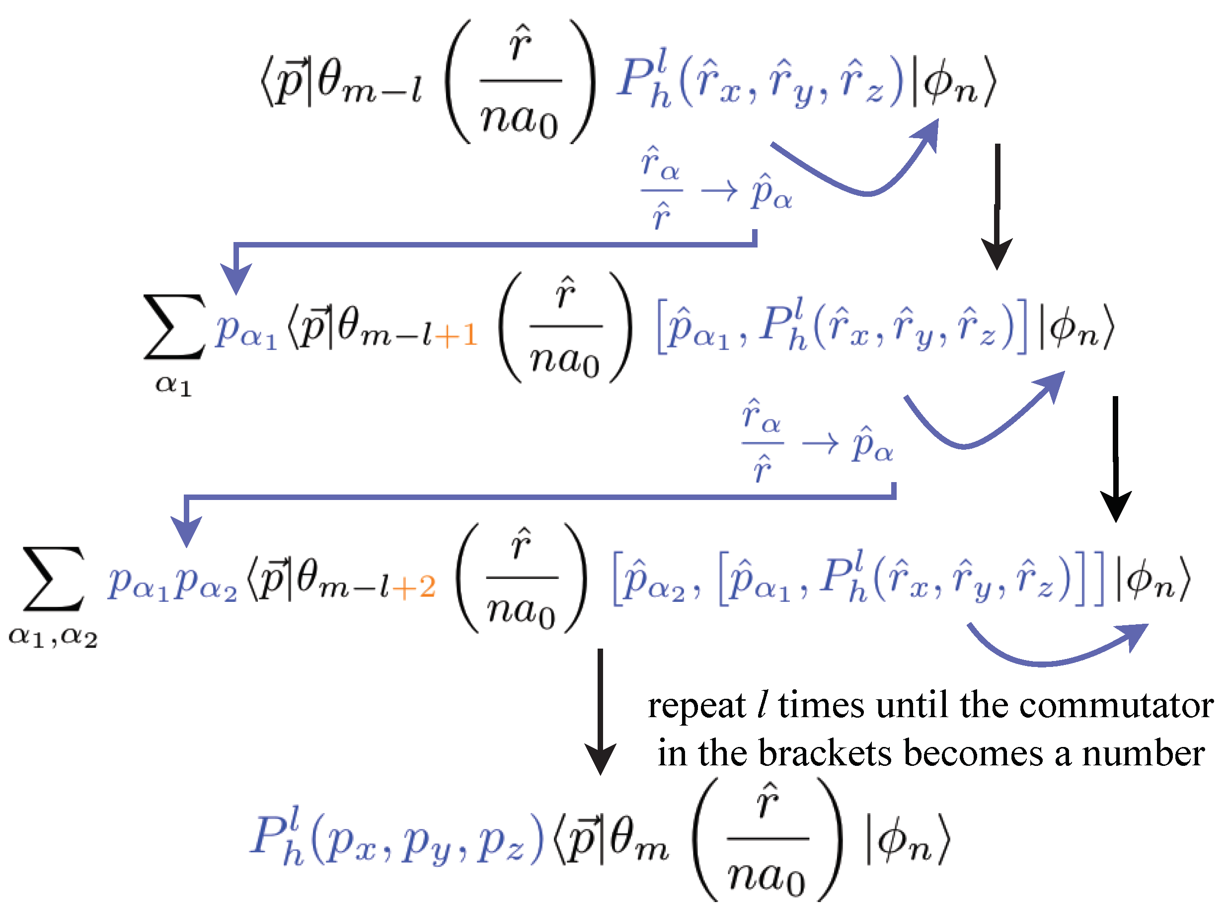
We repeat this procedure until we reach . Here, the nested commutators result in a number, because a power of is removed with each nesting. The wavefunction then becomes
which requires determining the expectation value of the polynomial. Note that the emergence of the harmonic polynomial as a function of the momenta is subtle. The multiple commutators sequentially remove every factor of in each term of the polynomial leaving behind the constant prefactor. This is then multiplied by the corresponding factors, which allow us to reconstruct the harmonic polynomial as a function of momentum as follows:
So, we have only the matrix element left to evaluate. Since we have already found the matrix elements for arbitrary powers of , we can then determine this result once we have an explicit formula for the polynomial.
The polynomial recurrence relation can be rewritten in terms of derivatives as follows:
This polynomial is a reverse Bessel polynomial [31], which satisfies
The proof can be done with or without calculus—it is identical, because times the commutator of the radial momentum operator with a power of the radial coordinate operator is the same as the derivative with respect to the radial coordinate operator. The base case has and from Equation (134) with . We next work with the derivative form and note that
Plugging this into the derivative relation in Equation (140) yields
We now change the summation indices. We let and . Then, we have
One can easily verify the sum over by induction (for fixed j) to show that
We easily see the base case is satisfied since both sides are . Assume it holds up to m, then after separating the sum for up to m and adding in the term with , we have
So, the polynomial becomes
which establishes that is the jth inverse Bessel polynomial. Note that the recurrence relation with derivatives in Equation (140) appears to be a new relation for the reverse Bessel polynomials (that is, it is not in [31]).
We now must return to the problem of determining the matrix element in Equation (133). We have already found that the result for can be expressed in terms of the reverse Bessel polynomial . This result can be immediately generalized to , which can be expressed in terms of a reverse Bessel polynomial . To be more concrete, consider the following:
Unfortunately, this approach does not produce simple results for other powers. What does produce simple results is matrix elements of reverse Bessel polynomials times harmonic polynomials. We now describe why. As we already saw in Equation (136), if we have an expectation value of a reverse Bessel polynomial in times a harmonic polynomial, then the recurrence relation continues to have a reverse Bessel polynomial times a harmonic polynomial until the recursion ends because there are no more terms left in the harmonic polynomial. Hence, instead of starting with a power times a harmonic polynomial, we can easily compute the result if we start from a reverse Bessel polynomial times a harmonic polynomial. This allows us to immediately write down the following identity, which is illustrated graphically in Figure 3:
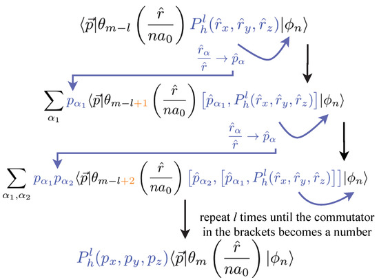
Figure 3.
Schematic for how to remove the harmonic polynomial from the operator matrix element to determine the wavefunction in momentum space. Here, is a reverse Bessel polynomial and is a harmonic polynomial.
We already know how to complete the calculation of those expectation values. We simply use the definition of the reverse Bessel polynomial in Equation (147) and the results for the expectation value of powers of the radial coordinate in Equations (115) and (117) to compute the final result. We find
It turns out that these complicated summations can be simplified, but they require some significant computation. Because we have not seen the details of this elsewhere, we present them here for completeness.
The innermost summation can be schematically written as follows:
with and suppressing constant factors with respect to the summand index k. This summation can be easily done. Simply use the binomial theorem to re-express the difference of two powers as follows:
because only terms with odd exponents contribute to the sum on the right-hand side of the top line (we changed in the second line). This completes the innermost summation.
The outermost sum becomes
This remaining sum can be performed exactly. We go through the details next. We start by investigating the summation
Since we can write the binomial expansion as
we see that the binomial coefficient in the summation in Equations (150) and (154) is the coefficient of the term, so that
where the contour for the integral encircles the origin and lies within a circle whose radius is smaller than . Summing the series gives
The only pole comes from (which is an order pole) and we find
Some simple algebra with the operators applied to the summation yields
Using this result, we find Equation (153) becomes
Taking the imaginary part of the term in the curly brackets yields
with . Clearly, only the coefficient of the term in the parenthesis will contribute. To isolate this term, we first note that for , which will hold for all v as , we have
Combining this with the binomial theorem, which says
for , we find the following: (i) when , the coefficient of is
(ii) when , the coefficient of is the coefficient of in
which implies with the coefficient being ; and (iii) when , there are no terms proportional to since the minimal power of x that appears is . Hence, we learn that Equation (161) is equal to . This simplification then allows us to conclude that
(recall that ). It is remarkable that one finds such a simple result for this complex expression!
We are now ready to work on the general case. We begin with the definition of the momentum-space wavefunction in Equation (108). The first step is to recognize that the term can be moved to the left, because it commutes with and . Then, the work in Section 2 and Section 3 showed that
where the left-hand side is not normalized, but the right-hand side is. We need to re-express this polynomial in in terms of an expansion with respect to reverse Bessel polynomials. Following [31], we can expand a polynomial of the form in terms of reverse Bessel polynomials via
where satisfies
with for . We need to expand the polynomial , so that we have
for . We next compute
Using this result, we find that satisfies
The sum can be performed by employing the well-known Van Der Monde convolution of binomial coefficients,
we break up the summation into two terms—one corresponding to and the other to . After summing the terms, we end up with
Putting this all together, we have
It turns out that this involves the properly normalized Gegenbauer polynomial, but it requires some additional work to show this.
The Gegenbauer polynomial satisfies
which follows from using its representation in terms of a hypergeometric function and simplifying the expression to put it into a form similar to the one we have already generated. This gives
The only remaining calculation is to find the normalized auxiliary Hamiltonian ground state wavefunction in momentum space. To do this, we use a translation operator to translate the momentum state at the origin to the state at . Hence,
Expanding in a power series, we have
First, we show that the matrix element vanishes when . To see this, we use the property that the auxiliary Hamiltonian ground state is annihilated by for all . Then, we directly compute
In general, we will show that all odd powers vanish. To see the general result, we consider the arbitrary case
The last line follows from the fact that all terms are proportional to : we get terms when the operator commutes with the terms with ; 3 more terms when it commutes with the operator; and then 1 more term from the last line. What this identity shows is that we can remove two operators at a time from the product, generating multiplied by numbers. If m is odd, we end with the term that has , which we already showed vanished. So, all odd powers give zero. If m is even, and is given by , then we find that the matrix element becomes
Substituting into the summation in Equation (179) yields
The sum is the derivative of the geometric series, so we finally obtain
Because the harmonic polynomial is normalized when integrated over the angular coordinates, we choose the normalization constant to satisfy
or
The final momentum space wavefunction becomes
which is the conventional result for the momentum-space wavefunction of Hydrogen.
We conclude this quite technical section with some thoughts. It is in many respects quite amazing that one can derive the momentum wavefunction algebraically, when none of the operators that appear in the operator expression of the wavefunction can be evaluated in terms of eigenvalues when they operate on momentum eigenstates. Nevertheless, using just the commutation relations and the fundamental properties of the auxiliary Hamiltonian ground states, we can completely construct them. In many respects, the hardest part of the challenge is rearranging the results to fit into the standard formulas for the polynomial representations used in the standard treatment of these wavefunctions. Yes, the algebra is lengthy, but we find it remarkable that all of this information is encoded within the commutation relations themselves (and the existence of position and momentum-space eigenfunctions at the origin).
5. The Conventional Confluent Hypergeometric Equation Approach
In this section, we relax the condition of not using calculus, and focus on how one can derive the conventional differential equation that the wavefunctions satisfy. The approach will also be based heavily on operator algebra, but it follows closely the differential equation approach used to solve the Hydrogen atom in a Cartesian coordinate basis [7]. Because of the additional complications one encounters in formulating a differential equation in momentum space, we forgo examining that problem here.
The ansatz for deriving the differential equation is that the wavefunction can be written in the following factorized form
where is the auxiliary Hamiltonian ground state, which satisfies . At this stage, we do not yet require the parameter to be a positive integer. Our goal is to find a differential equation for . This turns out to be rather straightforward, given the operator identities we have already developed. However, before proceeding too far, we need to discuss one technical detail. We assume that can be expressed as a power-series expansion. In this case, it is straightforward to note that
where the operator derivative notation above simply means that if , then .
Now, we simply operate onto and force the equation to satisfy an eigenvalue/eigenvector relationship. Hence, writing the Hamiltonian in terms of the kinetic and potential-energy pieces , we find the potential term commutes with the functions of coordinate operators and we obtain
We examine each term in turn. First, since commutes with , we have
This operator acts on . Using the fact that and Equation (33) gives
We use Equation (37) to evaluate the second term, which yields
The third term becomes
Assembling these three terms gives
For the state to be an eigenvector, we need the object in the curly brackets to vanish. It turns out this is the standard confluent hypergeometric equation for the Hydrogen atom’s radial wavefunction, but to see this, we need to make the radial coordinate operator dimensionless. As before, we define . Then, one can immediately verify that the expression in the curly brackets becomes (after multiplying by and evaluating against a coordinate eigenstate )
This is the confluent hypergeometric equation for the Hydrogen atom. One can then solve this using the Frobenius method and reproduce the wavefunction we worked out using other techniques in Section 2.
6. Conclusions
In this work, we have presented the solution of the Hydrogen atom using a Cartesian operator factorization approach. While the calculation is lengthy, it has a number of interesting aspects to it. First, it shows how one can solve quantum mechanics problems in terms of sums of noncommuting factorizations. Second, it illustrates how one can find the wavefunctions in coordinate space and in momentum space employing the same methodology (although the algebra for one is more complex). Third, it demonstrates that one can solve these problems without spherical harmonics and purely algebraically. We feel it is remarkable that one can achieve all of these goals for both the energy eigenvalues and the wavefunctions.
This representation-independent formulation of operator mechanics can be applied more widely than just for Hydrogen. We have already employed it for determining spherical harmonics [32], for the particle-in-a-box [33], and for the simple-harmonic oscillator [34]; it can also be applied to other problems that can be solved analytically. Furthermore, operator mechanics provides a framework where one separates the determination of the energy eigenfunctions from the calculation of the wavefunctions in coordinate or momentum space; this representation-independent approach places quantum mechanics in a more elegant mathematical setting and completes the development initiated by Pauli, Dirac, and Schrödinger at the dawn of quantum mechanics.
Author Contributions
Conceptualization, J.K.F.; methodology J.K.F. and X.L.; validation, X.L.; formal analysis, C.D., J.K.F. and X.L.; writing, C.D., J.K.F. and X.L.; visualization, J.K.F. and X.L.; supervision, J.K.F.; funding acquisition, C.D., J.K.F. and X.L. All authors have read and agreed to the published version of the manuscript.
Funding
This research was funded by the National Science Foundation under grants numbered PHY-1620555 and PHY-1915130. J.K.F. was also supported at Georgetown University by the McDevitt bequest. X.L. was supported by the Global Science Graduate Course (GSGC) program of the University of Tokyo for the later parts of this work. C.D. was supported by the National Science Foundation under grant number DMR-1747426 for the later parts of this work.
Institutional Review Board Statement
Not applicable.
Informed Consent Statement
Not applicable.
Data Availability Statement
Not applicable.
Acknowledgments
We learned about the Cartesian factorization from Barton Zwiebach via the MIT 8.05x MOOC. He learned it from Roman Jackiw. We thank Jolyon Bloomfield from MIT and Tianlalu from StackExchange for help in deriving the identity in Equation (166).
Conflicts of Interest
The authors declare no conflict of interest.
Appendix A. Algebraic Derivation of the Ground-State Wavefunction in the Coordinate Representation
In principle, we can go through a similar procedure as we did for deriving the momentum wavefunction that computes the coordinate wavefunction employing operators in Cartesian space. However, the derivation becomes painful and torturous (and this paper has already a lot of long algebra in it). If, on the other hand, we derive the formulas employing the radial momentum operator to translate the radial coordinate, the calculation becomes much simpler. We provide a quick sketch of this approach here.
The one ansatz we make is that this ground-state wavefunction is a function of r only. Then, a straightforward analysis with the radial momentum operator [22] shows that we can write the radial coordinate eigenstate as
Note that this is a highly nontrivial relation that could not be guessed. It follows from systematically changing coordinates from a Cartesian system to a spherical system and applying those coordinate changes to the conventional translation operator. Details are provided elsewhere [22]. The apparent singularity as is needed to cancel a similar singularity that arises from the radial momentum operator.
Using this result, we have immediately that
Now, we expand in a power series
and note that
This simple result allows us to compute all powers immediately. Next, we perform the sum and immediately find that
which produces the correct wavefunction up to the normalization constant, that we already discussed in the main text.
References
- Pauli, W. Über das Wasserstoffspektrum vom Standpunkt der neuen Quantenmechanik. Z. Phys. 1926, 36, 336–363. [Google Scholar] [CrossRef]
- Schrödinger, E. Quantisierung als Eigenwertproblem I. Ann. Phys. (Leipzig) 1926, 384, 361–376. [Google Scholar] [CrossRef]
- Schrödinger, E. Quantisierung als Eigenwertproblem II. Ann. Phys. (Leipzig) 1926, 384, 489–527. [Google Scholar] [CrossRef]
- Schrödinger, E. A Method of Determining Quantum-Mechanical Eigenvalues and Eigenfunctions. Proc. R. Irish Acad. Sec. A Math. Phys. Sci. 1940, 46, 9–16. [Google Scholar]
- Schrödinger, E. Further Studies on Solving Eigenvalue Problems by Factorization. Proc. R. Irish Acad. Sec. A Math. Phys. Sci. 1940, 46, 183–206. [Google Scholar]
- Infeld, L.; Hull, T.E. The Factorization Method. Rev. Mod. Phys. 1951, 23, 21–68. [Google Scholar] [CrossRef]
- Fowles, G.R. Solution of the Schrödinger equation for the hydrogen atom in rectangular 283 coordinates. Am. J. Phys. 1962, 30, 308–309. [Google Scholar] [CrossRef]
- Stone, M.H. Linear Transformations in Hilbert Space. III. Operational Methods and Group Theory. Proc. Natl. Acad. Sci. USA 1930, 16, 172–175. [Google Scholar] [CrossRef] [PubMed] [Green Version]
- von Neumann, J. Die Eindeutigkeit der Schrödingerschen Operatoren. Math. Ann. 1931, 104, 570–578. [Google Scholar] [CrossRef]
- Harris, L.; Loeb, A.L. Introduction to Wave Mechanics; McGraw-Hill: New York, NY, USA, 1963. [Google Scholar]
- Green, H.S. Matrix Mechanics; P. Noordhoff Ltd.: Grönigen, The Netherlands, 1965. [Google Scholar]
- Bohm, A. Quantum Mechanics Foundations and Applications, 3rd ed.; Springer Inc.: New York, NY, USA, 1993. [Google Scholar]
- Ohanian, H.C. Principles of Quantum Mechanics; Prentice Hall: New York, NY, USA, 1989. [Google Scholar]
- Ode Lange, L.; Raab, R.E. Operator Methods in Quantum Mechanics; Oxford Science Series; Oxford Science: Oxford, UK, 1992. [Google Scholar]
- Hecht, K.T. Quantum Mechanics; Springer Inc.: New York, NY, USA, 2000. [Google Scholar]
- Binney, J.; Skinner, D. The Physics of Quantum Mechanics; Oxford University Press: Oxford, UK, 2014. [Google Scholar]
- Schwabl, F. Quantum Mechanics, 4th ed.; Springer Inc.: New York, NY, USA, 2007. [Google Scholar]
- Razavy, M. Heisenberg’s Quantum Mechanics; World Scientific Publishing Co.: Singapore, 2011. [Google Scholar]
- Judd, B.R. Angular Momentum Theory for Diatomic Molecules; Academic Press: New York, NY, USA, 1975. [Google Scholar]
- Fock, V. Zur Theorie des Wasserstoffatoms. Z. Phys. 1935, 98, 145–154. [Google Scholar] [CrossRef]
- Andrianov, A.A.; Borisov, N.V.; Ioffe, M.V. The factorization method and quantum systems with equivalent energy spectra. Phys. Lett. 1984, 105A, 19–22. [Google Scholar] [CrossRef]
- Rushka, M.; Esrick, M.A.; Mathews, W.N., Jr.; Freericks, J.K. Converting translation operators into plane polar and spherical coordinates and their use in determining quantum-mechanical wavefunctions in a representation-independent fashion. J. Math. Phys. 2021, 62, 072102. [Google Scholar] [CrossRef]
- Dirac, P.A.M. The elimination of the nodes in quantum mechanics. Proc. R. Soc. Lond. Ser. A Math. Phys. 1926, 111, 281. [Google Scholar]
- Kramers, H.A. Quantum Mechanics; North-Holland: Amsterdam, The Netherlands, 1957. [Google Scholar]
- Brinkman, H.C. Applications of Spinor Invariants in Atomic Physics; North-Holland: Amsterdam, The Netherlands, 1956. [Google Scholar]
- Powell, J.L.; Crasemann, B. Quantum Mechanics; Addison-Wesley: New York, NY, USA, 1961. [Google Scholar]
- Weinberg, S. Lectures on Quantum Mechanics; Cambridge University Press: Cambridge, UK, 2012. [Google Scholar]
- Avery, J.S. Harmonic polynomials, hyperspherical harmonics, and atomic spectra. J. Comp. Appl. Math. 2010, 233, 1366–1379. [Google Scholar] [CrossRef] [Green Version]
- Schiff, L.I. Quantum Mechanics; McGraw-Hill: New York, NY, USA, 1949. [Google Scholar]
- Paz, G. The non-self-adjointness of the radial momentum operator in n dimensions. J. Phys. A Math. Gen. 2002, 35, 3727. [Google Scholar] [CrossRef] [Green Version]
- Grosswald, E. Bessel Polynomials; Dold, A., Eckmann, B., Eds.; Lecture Notes in Mathematics; Springer Inc.: New York, NY, USA, 1978; Volume 698. [Google Scholar]
- Weitzman, M.; Freericks, J.K. Calculating spherical harmonics without derivatives. Condens. Matter Phys. 2018, 21, 33002. [Google Scholar] [CrossRef] [Green Version]
- Jacoby, J.A.; Curran, M.; Wolf, D.R.; Freericks, J.K. Proving the existence of bound states for attractive potentials in one-dimension and two-dimensions without calculus. Eur. J. Phys. 2019, 40, 045404. [Google Scholar] [CrossRef] [Green Version]
- Rushka, M.; Freericks, J.K. A completely algebraic solution of the simple harmonic oscillator. Am. J. Phys. 2020, 88, 976–985. [Google Scholar] [CrossRef]
Publisher’s Note: MDPI stays neutral with regard to jurisdictional claims in published maps and institutional affiliations. |
© 2022 by the authors. Licensee MDPI, Basel, Switzerland. This article is an open access article distributed under the terms and conditions of the Creative Commons Attribution (CC BY) license (https://creativecommons.org/licenses/by/4.0/).