Abstract
Stellar parameters are estimated through spectra and are crucial in studying both stellar evolution and the history of the galaxy. To extract features from the spectra efficiently, we present ESNet (encoder selection network for spectra), a novel architecture that incorporates three essential modules: a feature encoder (FE), feature selection (FS), and feature mapping (FM). FE is responsible for extracting advanced spectral features through encoding. The role of FS, on the other hand, is to acquire compressed features by reducing the spectral dimension and eliminating redundant information. FM comes into play by fusing the advanced and compressed features, establishing a nonlinear mapping between spectra and stellar parameters. The stellar spectra used for training and testing are obtained through crossing LAMOST and SDSS. The experimental results demonstrate that for low signal-to-noise spectra (0–10), ESNet achieves excellent performance on the test set, with mean absolute error (MAE) values of 82 K for (effective temperature), 0.20 dex for (logarithm of the gravity), and 0.10 dex for (metallicity). The results indeed indicate that ESNet has an excellent ability to extract spectral features. Furthermore, this paper validates the consistency between ESNet predictions and the SDSS catalog. The experimental results prove that the model can be employed for the evaluation of stellar parameters.
1. Introduction
With the advancement of spectroscopic surveys, a vast amount of stellar spectra have been acquired. The SEGYE plan by SDSS involved sampling stars from different distances to capture spatial substructures in the Galactic stellar halo [1]. The Anglo-Australian Observatory utilized the Schmidt telescope to determine the radial velocity and parameters of stars [2]. LAMOST launched its low-resolution spectral survey in 2012, amassing over 10 million spectra with R=1800 (wavelength range 3690–9100 Å) [3]. SDSS’s APOGEE project focused on investigating Red Giants, and it provided spectra with R = 22,500 (wavelength range 3800–9200 Å) [4]. Gaia-ESO obtained approximately 100,000 stellar spectra (wavelength range 3700–9000 Å), providing valuable kinematic and elemental abundance data [5]. From the spectra, important information such as the age, temperature, and metal abundances (Fe, Mg, Al, etc.) of the objects can be extracted, which is significant for the study of celestial evolution and the understanding of the history of galaxies [6,7,8,9].
Traditionally, stellar parameters were determined by comparing observed spectra with spectral templates. For instance, Elsner introduced a weighted nearest neighbor template matching method [10]. Meanwhile, the equivalent width method is a traditional method for stellar parameters’ and chemical abundances’ determination [11]. There are also some other methods, such as MOOG [12] and SME [13]. However, traditional methods demand high-quality spectra.
An alternative mathematical approach was employed to evaluate the stellar parameters, specifically utilizing line indices. This method established a nonlinear mapping relation between the spectral line features and the stellar parameters, such as the new Lick Balmer index [14], the Rose index [15], and the SDDD-based Lick/SDSS index [16]. However, the line indices method also necessitates high-quality spectra (SNR > 20) to produce reliable outcomes.
With the advancements in machine learning, processing vast quantities of spectra in bulk has become feasible. For instance, Cannon utilized data-driven approaches to evaluate stellar parameters like (effective temperature), (logarithm of the gravity), and metal abundances ( (metallicity)) for stars [17]. Cannon2 evaluated , , and 15 elemental abundances (C, Mg, Al, etc.) of Red Giants [18]. CNN-based neural networks were also employed to measure stellar parameters (, , ) by using a synthetic training set [19]. There were some methods that used observed data for the training (as in the current study), such as [20,21]. Additionally, some parametric regression models based on traditional regression methods to evaluate (, , ), such as SLAM [22] and SCDD [23], were proposed. Ref. [24] played a pioneering role in employing neural networks to estimate stellar , , and across various SNR and spectral resolutions, encompassing even very low-resolution spectra. Similarly, ref. [25] introduced deep learning networks to predict stellar parameters using SDSS spectra, while ref. [26] concentrated on LAMOST DR5 spectra and introduced generative spectrum networks for stellar parameter estimation.
For low SNR spectra, it has been a challenge to extract effective features from them to estimate stellar parameters. Based on machine learning methods, both refs. [27,28] estimate stellar parameters for low SNR spectra, but the results are not satisfactory for SNRs between 0 and 10.
Existing methods cannot effectively remove spectral redundant information (mainly includes noise, features that are not sensitive to stellar parameters) and extract spectral features from low SNR spectra. Thus, this paper proposes ESNet (encoder selection network for spectra), as a new approach to evaluating stellar parameters.
2. Data
This section provides a detailed description of the data used in this paper, which includes information about its sources, the criteria used for selection, and the pre-processing steps.
2.1. Sources
Data are from LAMOST and SDSS. LAMOST provides spectra, and SDSS provides stellar parameters.
2.1.1. LAMOST Survey
LAMOST [29] currently provides spectra for approximately one million objects, encompassing stars, galaxies, and quasars. These spectra offer crucial information concerning the physical properties, chemical composition, and motions of these objects. The wavelength range covered by the LAMOST spectra spans from 3690 to 9100 Å, and the spectra have a resolution of R 1800 [30]. In one of its data releases, LAMOST DR10, around eleven million low-resolution spectra were made available, with stellar spectra accounting for 97.1% of the total number. Among these stellar spectra, approximately 7.4 million are utilized for the evaluation of stellar parameters.
2.1.2. SDSS Survey
SDSS [31] houses an extensive collection of astronomical data, spanning a vast region of the sky. These data include essential information such as the position, brightness, and spectral details of billions of celestial objects, along with their physical properties. SDSS also offers a wide range of data, including images, galaxy redshift measurements, galaxy photometry, and a comprehensive catalog of sky survey objects. Additionally, the wavelength range covered by the SDSS DR17 APOGEE spectra with a resolution of R 22500 [32] spans from 3800 to 9200 Å, and high-quality atmospheric parameters [, , , ] are provided. Estimating atmospheric parameters using high-resolution spectra is more accurate [28]. Thus, in the paper, APOGEE’s labels are used. The APOGEE Stellar Parameter and Chemical Abundances Pipeline (ASPCAP) [33] is a software pipeline for the analysis of stellar spectra, mainly used to process spectra from the Apache Point Observatory Galactic Evolution Experiment (APOGEE). ASPCAP aims to extract stellar parameters (e.g., , , metal abundances, etc.) and chemical abundances (e.g., elemental abundances) from stellar spectra.
2.2. Selection
Spectra that have a spherical distance less than 3 arcsec are considered to belong to the same target source, and this criterion is used for the selection of spectra [34]. The data are obtained by cross-matching the LAMOST data with SDSS data using the Tool for Operations on Catalogs and Tables (TOPCAT) [35]. The spectra are then further selected based on the following limitations [23]: (1) ; (2) ; (3) ; (4) < 200; (5) < 0.1; (6) < 0.1. After applying these selection criteria, there are a total of 129,108 spectra available for training and testing.
2.3. Pre-Processing
To enhance the usability of spectral information, proper processing of stellar spectra is necessary, especially considering the impact of extinction and instrument noise [28]. The specific details of the processing steps are as follows:
(1) Converting wavelength provided by LAMOST to rest frame. This will eliminate the effect of the radial velocity on spectra, as shown in Equation (1).
where is the wavelength in the rest frame, is the wavelength provided by LAMOST, is the radial velocity, and C is the speed of light.
(2) Handling bad fluxes. Using the masks provided by LAMOST, the unreliable flux values are substituted with the corresponding continuum values, instead of being deleted.
(3) Resampling. To construct the dataset, the spectra are resampled by the spline interpolation method with a step of 0.0001 in logarithmic wavelength coordinates.
(4) Normalizing spectra. Due to the uncertainty in the flux calibration and unknown extinction values in the LAMOST stellar spectra, it is necessary to normalize the spectra. We map the spectral fluxes to values between 0 and 1, so that spectra can be compared and processed on the same scale. This normalization method is very suitable for machine learning.
where F is spectral flux, and is the normalized spectra.
3. Method
This section describes the network structure, including the feature encoder (FE) module, feature selection (FS) module, and feature mapping (FM) module.
3.1. Network Structure
This section provides a detailed description of the network structure, as depicted in Figure 1. ESNet is composed of three main modules: the FE module, the FS module, and the FM module. The FE module is constructed using an encoder architecture inspired by encoder–decoder. It encodes the spectra by mapping them to high-level features, thereby achieving dimension reduction. The encoder first encodes the original spectrum as a vector; to ensure that the vector can represent the original spectrum, the vector is then restored to the original spectrum by the decoder. The encoder and decoder consist of three linear layers, but their structures are symmetric. In Section 4.1, we compare the effect of whether the encoder uses convolutional layers or does not on the prediction results, and the results prove that the performance is better using only linear layers, which may be mainly due to the fact that the linear layers can pay sufficient attention to the features of the spectra. The FS module employs the LASSO method to extract spectral features and effectively remove redundant information from the spectra. The FM module is based on a Multi-Layer Perceptron (MLP) neural network. It combines the features extracted by the FE and FS modules and establishes a nonlinear mapping between the features and the stellar parameters. We compare the effects of different layers on the prediction results, and it is found that the performance is better when the FM module uses a four-layer structure. The main reason may be that the four-layer structure can sufficiently extract features while ensuring the generalization ability of the network.
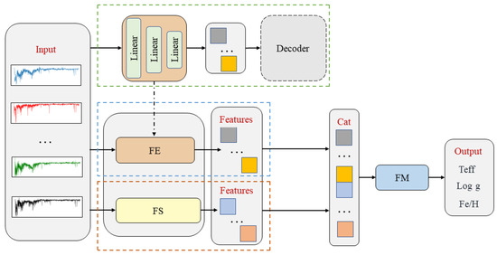
Figure 1.
The structure of the ESNet. It consists of FE module, FS module, and FM module. FE and FS are trained separately. Decoder works when training FE and does not participate in testing.
3.1.1. The FE Module
The FE module utilizes an encoder architecture inspired by encoder–decoder [36]. Encoder–decoder is a pair of interconnected modules commonly used in deep learning and neural networks for data transformation. The encoder takes the input data, such as spectra, and maps them to a higher-level representation space through a series of processing and transformation operations, effectively achieving dimensionality reduction. By doing so, the encoder captures essential features present in the input data and compresses them into a higher-level feature vector.
The decoder, on the other hand, performs the inverse process of the encoder. It takes the higher-level feature vector generated by the encoder and reconstructs the original data. The primary goal of the decoder is to restore the original data as accurately as possible, minimizing the difference between the reconstructed data and the original data.
During the training stage, the encoder is used to map the spectra into higher-level feature vectors, and then the decoder reconstructs the original spectra from these feature vectors. This means that the higher-level feature vectors effectively represent the essential information present in the original spectra. During the testing stage, only the encoder works, mapping the spectra into higher-level feature vectors.
By leveraging the encoder–decoder, the FE module is capable of capturing crucial spectral features and achieving effective dimensionality reduction.
3.1.2. The FS Module
The FS module utilizes the Least Absolute Shrinkage and Selection Operator (LASSO) method to select spectral features, eliminate redundant information, and reduce the dimensionality of the spectra.
LASSO is a statistical method employed for linear regression and feature selection [37]. It accomplishes model sparsity and variable selection by imposing constraints on the regression coefficients. The penalty function of LASSO involves minimizing the residual sum of squares (RSS) with an L1-norm penalty term. The expression of the penalty function is shown in the following equation:
where Y represents the regression term, stands for the input, represents the coefficient, and a is the adjustment parameter. By manipulating the parameter a, the overall regression coefficients can be compressed effectively. Through the utilization of the L1 parametric penalty term, some regression coefficients can be driven to zero, resulting in spectral dimension reduction and the elimination of redundant information.
As a result, redundant information in the spectra can be efficiently eliminated, while retaining spectral features that exhibit sensitivity to stellar parameters.
3.1.3. The FM Module
The FM, or feature mapping, is a crucial component in the ESNet, and it consists of a Multi-Layer Perceptron (MLP) [38]. The MLP is chosen for its exceptional ability to achieve high levels of parallel processing and its strong adaptive and self-learning functions, attributed to its highly nonlinear global action. As an artificial neural network model, MLP is one of the most fundamental models.
The typical architecture of MLP comprises an input layer, multiple hidden layers, and an output layer. The input layer receives the original data, while the hidden layers conduct nonlinear transformations and extract essential features from the input data. Finally, the output layer yields the ultimate result. By leveraging the power of MLP, the FM effectively maps the features extracted through FS and FE to the corresponding stellar parameters.
4. Results
This section describes the experiment and the results. Mean absolute error (MAE) is a statistical metric used to assess the average absolute difference between predicted values and actual observations. It is utilized to evaluate the accuracy of models in predicting outcomes. Thus, in this paper, MAE is employed as an evaluation metric.
4.1. Selection of Model Structure and Estimation of Model Uncertainty
In order to choose a better model structure, we conduct comparison experiments, and the results are shown in Table 1. Firstly, we compare the activation functions (ReLU, Logistic, and Tanh), and the best result is obtained by using Logistic; secondly, we compare the loss functions (L1loss and L2loss), and the experimental results show that the loss functions do not have a significant effect on the model performance. We also compare the effect of different numbers of layers of the FM, and the results show that the network is best when the number of layers is four. This may be because the network structure with three layers cannot fully extract the features, while the network with five layers can fully extract the features, but the generalization performance is not good.

Table 1.
Comparative experiments for selection of model structures.
For the encoder module, we compare the effect of using convolutional layers and not using them on the performance of the model, and the results show that the performance of the network without convolutional layers is better, which may be mainly due to the fact that the linear layer can focus on the global information of the spectra compared to the convolutional layer.
The uncertainty estimates for the model are shown in Table 2. First, we train eight models and then estimate the stellar parameters using each of the eight models on the test set. The variance in the predictions of the eight models is calculated as the model uncertainty [21]. The results are as follows: () = 49, () = 0.547; () = 0.07, () = 0.0008; () = 0.04, () = 0.0004.

Table 2.
The uncertainty estimates for the model.
4.2. Evaluation of Predictions
The dataset is partitioned into three subsets: a training set, a validation set, and a test set, distributed in an 8:1:1 ratio. We sample all the spectra uniformly to obtain the training set. The distribution of the spectral SNR for the training set is shown in Figure 2. The distribution of the number of , , in the training set is shown in Figure 3. Finally, the number of metal-poor stars is 181 (accounting for 0.2%). At training time, we process the in the labels by taking logarithms.

Figure 2.
Distribution of training samples along with SNR_g.
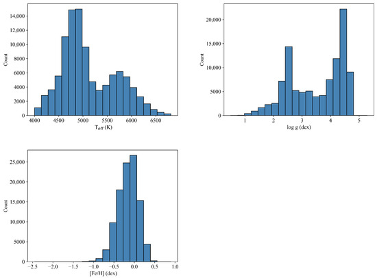
Figure 3.
The distribution of , , in the training set.
For the ESNet model, the spectra are used as inputs, while the corresponding stellar parameters serve as labels. Spectral features are extracted using the FE and FS modules. The features extracted by the FE and FS modules are fused. Subsequently, the FM maps the fused features to the stellar parameters.
The ESNet model’s performance is evaluated using the test set. The model’s predictions for the stellar parameters are compared against the labels (SDSS). The comparison between the ESNet’s predictions and the actual labels (SDSS) is shown in Figure 4. The comparison between the ESNet’s predictions and the actual labels (SDSS) using the color code with respect to the - diagram is shown in Figure 5. It is evident from the figure that the distribution of the ESNet’s predictions closely resembles that of the SDSS labels. It indicates that the ESNet model achieves promising results in predicting the stellar parameters.
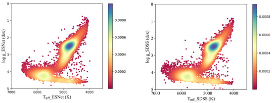
Figure 4.
The distribution diagram of the catalog on and . The left one is the ESNet predictions, and the right one is the labels (SDSS catalog). Color bar represents the density of data points with a change in color. Larger values on the color bar indicate greater density.
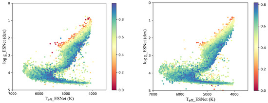
Figure 5.
The comparison between the ESNet predictions and the actual labels (SDSS) using color code with respect to the - diagram. The left one is the ESNet predictions, and the right one is the labels (SDSS catalog). Color bar represents the density of data points with a change in color. Larger values on the color bar indicate greater density.
The consistency between the ESNet predictions and the labels is thoroughly analyzed and evaluated. Scatter density plots for the stellar parameters , , and are presented in Figure 6, providing a visual representation of the relationship between the ESNet predictions and the labels.
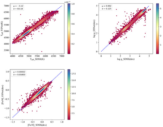
Figure 6.
Consistency between the prediction (ESNet) and SDSS catalog. The upper left figure refers to ; the upper right figure refers to ; the bottom left figure refers to . Color bar represents the density of data points with a change in color. Larger values on the color bar indicate greater density.
Additionally, histograms depicting the differences between the ESNet predictions and the labels are shown in Figure 7. The experimental results reveal that the diagonal distributions in the scatter density plots (Figure 6) align closely with the 45° line, indicating that there is no significant systematic deviation between the ESNet predictions and the labels, and the ESNet model exhibits good consistency in predicting the stellar parameters.
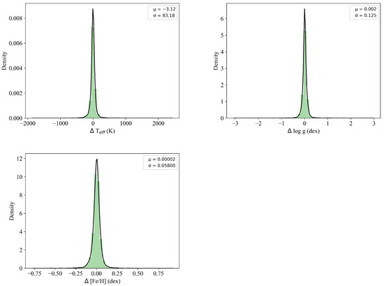
Figure 7.
Distribution of residual error between predictions and SDSS catalog. The upper left figure refers to ; the upper right figure refers to ; the bottom left figure refers to .
To further analyze the consistency, we calculate two statistical metrics: the mean value () and the mean square error () of the differences between the ESNet predictions and the labels for each stellar parameter (, , and ). The results are as follows: () = −3.12, () = 83.18; () = 0.002, () = 0.125; () = 0.00002, () = 0.05800.
However, we also note that the ESNet model performs relatively poorly for cold and hot stars. This limitation may be attributed to the lack of spectra for such stars in the SDSS catalog [28], since the stellar parameters in this paper are from the SDSS catalog, which weakens ESNet’s ability to take spectral features of both cool and hot stars; alternatively, the divergence between the two catalogs could potentially have a significant influence.
In conclusion, the analysis and statistical results provide strong evidence for the high and stable consistency between the ESNet predictions and the labels, validating the effectiveness of the proposed approach in estimating stellar parameters from spectra.
4.3. Comparing the LAMOST Catalog with the SDSS One
In order to further validate the accuracy and stability of the ESNet predictions, the paper conducts a comparison between the stellar parameters provided by LAMOST and SDSS. For this comparison, we utilize 12,910 spectra from the test set. The validation results are presented in Figure 8, which includes scatter density plots, and Figure 9, which displays statistical differences between the stellar parameters from LAMOST and SDSS.
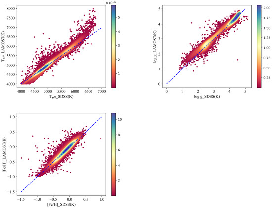
Figure 8.
Consistency between the LAMOST catalog and SDSS one. The upper left figure refers to ; the upper right figure refers to ; the bottom left figure refers to . Color bar represents the density of data points with a change in color. Larger values on the color bar indicate greater density.
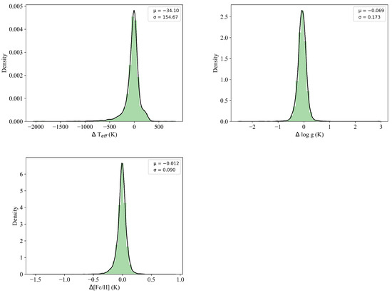
Figure 9.
Distribution of residual error between LAMOST catalog and SDSS one. The upper left figure refers to ; the upper right figure refers to ; the bottom left figure refers to .
We present scatter plots (Figure 8) of the three parameters in the test set, along with histograms of the errors. The scatter plots reveal notable differences between the stellar parameters , , and provided by LAMOST and those from SDSS, indicating a significant systematic deviation between the two catalogs. By comparing Experiment 4.1, we find that the ESNet predictions exhibit better agreement with the SDSS catalog than with the LAMOST catalog.
For the scatter plot (upper left) in Figure 8, we observe that the provided by SDSS for cool stars are generally higher than those from LAMOST, while, for hot stars, the from SDSS are relatively lower. The corresponding histogram reveals a systematic error of = −34.10 and a deviation of = 154.67 between the two catalogs concerning .
For the scatter plot (upper right) in Figure 8, a systematic error is evident between the two catalogs, primarily observed in within the range of (0, 2.5), with those from the SDSS catalog being smaller than those from LAMOST. The histogram illustrates a systematic error of = −0.069 and a deviation of = 0.173 for .
Regarding , the scatter plot (middle) in Figure 8 indicates an ambiguous systematic error. However, the dispersion between LAMOST and SDSS for is greater than the dispersion between the ESNet predictions and SDSS. The corresponding histogram presents a systematic error of = −0.012 and a dispersion of = 0.090 between the two catalogs.
In summary, the stellar parameters provided by LAMOST (, , ) show a significant systematic error when compared to the SDSS catalog.
Compared to the LAMOST and SDSS catalogs, the ESNet predictions exhibit higher consistency with the SDSS catalog. The systematic error and deviation of the ESNet predictions are lower than those (, , and ) provided by LAMOST. As a result, the ESNet model can offer stellar parameters that align more closely with the SDSS catalog. We should note that the more precise and accurate ESNET labels with respect to SDSS are simply due to the fact that SDSS labels are used for training.
4.4. Comparison with Other Methods
To evaluate the effectiveness of our approach, ESNet is compared with several other models, including SLAM [22], SCDD [23], StarN [27] (because its model’s name is the same as that in [19], we use StarN to refer to this model), StarNet [19], Catboost [39], Lasso-MLP [28], and DenseNet [40]. The experimental results are presented in Table 3.

Table 3.
Comparing the ESNet with other regression methods.
Based on the experimental results, the performance of the different models on the test set is as follows.
StarNet: Based on a CNN, the network structure consists of two convolutional layers and three linear layers. Data preprocessing: spectra are interpolated, resampled, and normalized. Training datasets and labels come from synthetic datasets. Limitations: for a low SNR (0–10), where the performance is 206, is 0.38, and is 0.13. However, due to its shallow network structure, StarNet struggles to effectively extract spectral features from spectra with information redundancy, leading to poor results when using the same dataset and labels as we did.
SLAM: The network structure consists of Support Vector Regression (SVR). Data preprocessing: spectra are normalized by dividing its pseudo-continuum, smoothed by smoothing spline, and resampled to the same wavelength grid. Training datasets and labels come from LAMOST. Limitations: when using the same dataset and labels as we did, for low SNR (0–10), where the performance is 111, is 0.33, and is 0.18. SLAM can partially extract spectral features, but its predictions for and are not satisfactory. The main reason might be SLAM’s limited ability to sufficiently extract the spectral features associated with and , when using the same dataset and labels as we did.
SCDD: Network structure consists of Catboost. Data preprocessing: spectra are divided into multiple windows and the statistical features of each window are extracted, e.g., mean, maximum, minimum, etc. Training datasets and labels come from LAMOST. Limitations: for low SNR (0–10), where the performance is 169, is 0.34, and is 0.15. SCDD splits the spectra into windows, extracts statistical features from each window to remove redundant information, and then fuses the features to train using Catboost. However, this approach causes the significant loss of valid spectral information, resulting in poor performance, when using the same dataset and labels as we did.
StarN: Based on a CNN, the network structure consists of two convolutional layers and three linear layers. Data preprocessing: spectra are resampled and normalized. Training datasets and labels come from a synthetic dataset and LAMOST. Limitations: for low SNR (0–10), where the performance is 257, is 0.36, and is 0.17. SCDD splits the spectra into windows, extracts statistical features from each window to remove redundant information, and then fuses the features to train using Catboost. Despite increasing the size of the convolution kernel, due to its shallow network structure, StarN struggles to effectively extract spectral features from spectra with information redundancy, leading to poor results, when using the same dataset and labels as we did.
Catboost: Network structure consists of Catboost. Data preprocessing: spectra are normalized by dividing its pseudo-continuum, smoothed by smoothing spline, and resampled to the same wavelength grid. Training datasets and labels come from LAMOST. Limitations: for a low SNR (0–10), where the performance is 157, is 0.26, and is 0.12. Unlike SCDD, this method directly trains Catboost by using spectra without removing redundant spectral information. Despite this, it outperforms SCDD, indicating that SCDD’s removal of valid spectral information hampers its performance, when using the same dataset and labels as we did.
Lasso-MLP: Network structure consists of Lasso and MLP. Data preprocessing: spectra are interpolated, resampled, and normalized. Training datasets and labels come from LAMOST and Payne catalogs. Limitations: for a low SNR (0–10), where the performance is 93, is 0.21, and is 0.12. For low SNR spectra, the LASSO method does not adequately extract spectral features and some features may be lost. The lost features are important in estimating the .
DenseNet: Based on a CNN, the network structure mainly consists of three dense blocks and two transition blocks. Data preprocessing: spectra are interpolated, resampled, and normalized to the range [0, 1]. Training datasets and labels come from LAMOST. Limitations: for low SNR (0–10), where the performance is 145, is 0.36, and is 0.15 on the test set. DenseNet proposes a new network structure with increased depth to extract spectral features. It shows some effectiveness compared with StarNet, but redundant information in the spectra can interfere with its feature extraction capability, when using the same dataset and labels as we did.
ESNet: For low SNR (0–10), where the performance is 82, is 0.20, and is 0.10. This method effectively removes redundant spectral information while retaining essential spectral features, and improves the performance compared to the other methods.
4.5. Validation of ESNet Using Other Catalogs
We cross the data with the Payne catalog [41] and obtain 248 spectra (SNR 0–10) and 968 spectra (SNR 10–20). At the same time, we estimate their stellar parameters and the results are shown in Table 4. Compared to other methods, ESNet performs best. Here, the performance is 146, is 0.17, and is 0.10 for SNR (0–10).

Table 4.
Comparison of predicted results with Payne catalog.
To further validate the ESNet in estimating stellar parameters using low SNR spectra, we cross it with 2MASS [42] through SIMBAD and obtain 190 (SNR 0–10) and 872 (SNR 10–20) spectra, and the experimental results are shown in Table 5. Compared to other methods, ESNet also performs best. The performance is 101, is 0.19, and is 0.11 for SNR (0–10).

Table 5.
Comparison of predicted results with 2MASS.
In summary, the experimental results demonstrate that ESNet, with its ability to remove redundant spectral information while retaining crucial features, outperforms the other models, offering more accurate and reliable predictions for stellar parameters on the test set.
5. Discussion
In this paper, we conduct a further investigation into the effect of the spectral SNR on stellar parameters, as depicted in Figure 10. The experimental results clearly demonstrate that the SNR significantly impacts the predictions of stellar parameters. Specifically, higher SNR values lead to more accurate predictions with reduced dispersion. Conversely, lower SNR values result in less accurate stellar parameter predictions with increased dispersion.
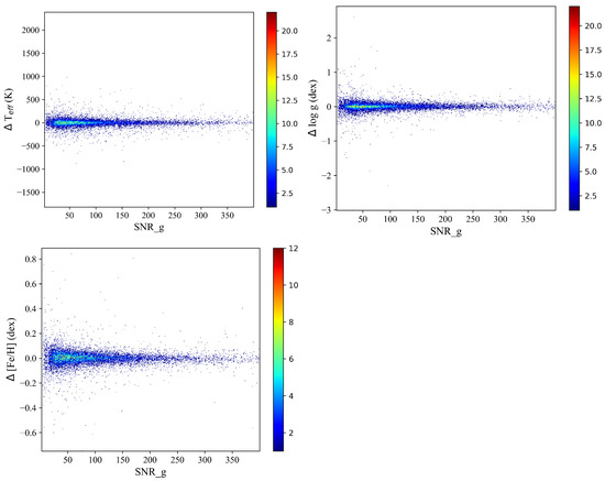
Figure 10.
The relationship between residual error and SNR. The upper left figure refers to ; the upper right figure refers to ; the bottom left figure refers to . Color bar represents the density of data points with a change in color. Larger values on the color bar indicate greater density.
We analyze the distribution of the SNR in the test set and find that the largest number of spectra fall within the SNR range of 0 to 200, as illustrated in Figure 11.
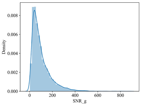
Figure 11.
Distribution of the number of spectra with respect to the SNR_g.
We explore the impact of the SNR on stellar parameters (, , ). Comparing the predictions to the SDSS catalog, we observe that the differences are smaller than those between LAMOST and SDSS. Specifically, for , the MAE of the former steadily decreases and converges with increasing SNR, while the latter also exhibits a tendency to converge, although with less stability.
For , the MAE of the former consistently decreases and converges as the SNR increases. On the other hand, the MAE of the latter also converges, but at a higher value, indicating larger errors.
Regarding , the MAE of the former continuously decreases and converges with increasing SNR. In contrast, the latter does not show a clear trend of convergence, displaying a diffused and unstable pattern, as depicted in Figure 12.
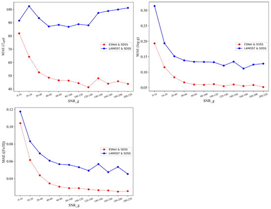
Figure 12.
The consistencies between ESNet predictions, LAMOST catalog, and SDSS catalog. The upper left figure refers to ; the upper right figure refers to ; the bottom left figure refers to .
These findings highlight the significance of the SNR in influencing the accuracy and stability of stellar parameter predictions, with higher SNR values leading to more precise and reliable results.
Additionally, we explore the influence of the SNR on the dispersion . The results indicate that the dispersion between the predictions (including , , ) and the SDSS catalog is smaller than the dispersion between LAMOST and SDSS. The experimental findings demonstrate a higher level of consistency between the predicted stellar parameters and the SDSS catalog, indicating the better stability of ESNet, as illustrated in Figure 13.
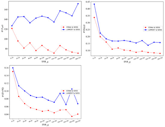
Figure 13.
The dispersion of the difference between SDSS catalog and ESNet predictions or LAMOST catalog. The upper left figure refers to ; the upper right figure refers to ; the bottom left figure refers to .
Specifically, for , the dispersion of the former steadily decreases and converges with the increase in SNR. The latter also exhibits a tendency to converge, but with less stability compared to the former. It can be found that there are some jumps observed in the ESNet red curve for . The main reason is that ESNet has a few values with large prediction errors at the jumps (in Figure 10), but even so, the dispersion of ESNet is still smaller than that of the LAMOST catalog.
Concerning , the dispersion of the former steadily decreases and converges as the SNR increases. Similarly, the latter also shows convergence, but the final convergence value is higher, indicating larger errors.
Regarding , the dispersion of the former consistently decreases and converges with increasing SNR. However, the latter does not display a clear trend of convergence, and the pattern is diffused and unstable.
The experimental results reveals that the SNR significantly impacts the stability of ESNet, leading to improved consistency and accuracy between the predicted stellar parameters and the SDSS catalog compared to LAMOST. The results underscore the robustness and reliability of ESNet in estimating stellar parameters.
The FE module in ESNet allows it to provide features that are compressed, as shown in Figure 14. It can be found that different parameters correspond to different spectral features. The FE indeed compresses the spectra and extracts spectral features that are sensitive to the parameters. For example, (1) some spectral lines (, and ) play an important role in estimating , and . (2) Some atomic metal lines (, , , , , ) are also critical in estimating , and . (3) At the same time, we note that contributes more to estimating and than to .
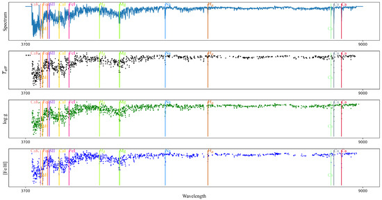
Figure 14.
Compressed feature figure obtained by compressing spectra through FE. Spectral features sensitive to atmospheric parameters are shown in the figure.
6. Conclusions
In this paper, we propose an ESNet for the estimation of stellar parameters (, , and ). Our approach utilizes stellar spectra common to both LAMOST and SDSS as the datasets, with spectra obtained from LAMOST and labels (stellar parameters) from SDSS. The experimental results demonstrate that the ESNet predictions align well with those of the SDSS catalog. For a low SNR (0–10), ESNet achieves impressive performance, with predictions of at 82 K, at 0.20 dex, and at 0.10 dex in the test set, which proves that ESNet has an excellent ability to extract spectral features and remove redundant information in spectra. Additionally, we explore the consistency between the SDSS and LAMOST catalogs, revealing errors of 92 K, 0.31 dex, and 0.12 dex for the three parameters, respectively. Compared to the results in Section 4, the ESNet predictions demonstrate improved consistency with the SDSS catalog compared to the LAMOST catalog.
To evaluate the proposed model, we compare it with seven methods. The results indicate that ESNet exhibits robust and better performance. At the same time, for a low SNR (0–10), compared to the Payne catalogs, ESNet achieves good performance, with predictions of at 146 K, at 0.17 dex, and at 0.10 dex. Compared to 2MASS, ESNet achieves good performance, with predictions of at 101 K, at 0.19 dex, and at 0.11 dex. The model’s stability is also analyzed, indicating that ESNet displays better robustness. Furthermore, we investigate the effect of the SNR on the predictions and find that as the SNR increases, ESNet exhibits better convergence and stability.
However, ESNet does not perform as well in extracting the spectral features of cool and hot stars, which proves that ESNet’s effectiveness in handling small data samples needs to be strengthened. Moreover, the performance in extracting low SNR spectral features is not as strong as the high SNR performance.
In conclusion, we will improve the model’s ability to extract spectral features with small data samples (hot and cool stars) and low SNR spectra in the next stage. In the future, 4MOST and SDSS-V will provide a large number of spectra that can be analyzed to reveal the properties and evolution of stars, galaxies, and the universe. It will be possible for ESNet to use these spectra to estimate the parameters.
Author Contributions
Methodology, K.W.; data curation, K.W.; writing—original draft preparation, K.W.; writing—review and editing, B.Q., A.-l.L., F.R. and X.J.; supervision, B.Q., A.-l.L., F.R. and X.J.; project administration, B.Q.; funding acquisition, B.Q. All authors have read and agreed to the published version of the manuscript.
Funding
This research was funded by the Natural Science Foundation of Tianjin, 22JCYBJC00410, and the Joint Research Fund in Astronomy, National Natural Science Foundation of China, U1931134.
Data Availability Statement
We are grateful to LAMOST for providing us with the data and SDSS for providing us with the stellar parameters. LAMOST DR10 Website: http://www.lamost.org/dr10/v1.0/ (accessed on 20 April 2023) and SDSS DR17 Website: https://www.sdss.org/dr17/ (accessed on 20 April 2023) and SIMBAD Website: http://simbad.u-strasbg.fr/simbad/ (accessed on 25 April 2023).
Acknowledgments
Sofware: Pytorch [43], Scipy [44], Matplotlib [45], Astropy [46].
Conflicts of Interest
The authors declare no conflict of interest.
References
- Ivezic, Z.; Schlegel, D.; Uomoto, A.; Bond, N.; Snedden, S. SDSS spectroscopic survey of stars. Mem. Della Soc. Astron. Ital. 2007, 77, 1057. [Google Scholar] [CrossRef]
- Steinmetz, M.; Zwitter, T.; Siebert, A.; Watson, F.G.; Freeman, K.C.; Munari, U.; Campbell, R.; Williams, M.; Seabroke, G.M.; Wyse, R.F.; et al. The radial velocity experiment (RAVE): First data release. Astron. J. 2006, 132, 1645. [Google Scholar] [CrossRef]
- Zhao, G.; Zhao, Y.H.; Chu, Y.Q.; Jing, Y.P.; Deng, L.C. LAMOST spectral survey—An overview. Res. Astron. Astrophys. 2012, 12, 723. [Google Scholar] [CrossRef]
- Cunha, K.; Smith, V.V.; Johnson, J.A.; Bergemann, M.; Mészáros, S.; Shetrone, M.D.; Souto, D.; Prieto, C.A.; Schiavon, R.P.; Frinchaboy, P.; et al. Sodium and oxygen abundances in the open cluster NGC 6791 from APOGEE H-band spectroscopy. Astrophys. J. Lett. 2015, 798, L41. [Google Scholar] [CrossRef]
- Gilmore, G.; Randich, S.; Asplund, M.; Binney, J.; Bonifacio, P.; Drew, J.; Feltzing, S.; Ferguson, A.; Jeffries, R.; Micela, G.; et al. The Gaia-ESO public spectroscopic survey. Messenger 2012, 147, 25–31. [Google Scholar]
- Si, J.M.; Luo, A.L.; Wu, F.Z.; Wu, Y.H. Searching for Rare Celestial Objects Automatically from Stellar Spectraof the Sloan Digital Sky Survey Data Release Eight. Spectrosc. Spectr. Anal. 2015, 35, 834–840. [Google Scholar]
- Santos, N.; Sousa, S.; Mortier, A.; Neves, V.; Adibekyan, V.; Tsantaki, M.; Mena, E.D.; Bonfils, X.; Israelian, G.; Mayor, M.; et al. SWEET-Cat: A catalogue of parameters for Stars With ExoplanETs-I. New atmospheric parameters and masses for 48 stars with planets. Astron. Astrophys. 2013, 556, A150. [Google Scholar] [CrossRef]
- Torres, G.; Andersen, J.; Giménez, A. Accurate masses and radii of normal stars: Modern results and applications. Astron. Astrophys. Rev. 2010, 18, 67–126. [Google Scholar] [CrossRef]
- Matteucci, F. Modelling the chemical evolution of the Milky Way. Astron. Astrophys. Rev. 2021, 29, 5. [Google Scholar] [CrossRef]
- Elsner, B.; Bastian, U.; Liubertas, R.; Scholz, R. Stellar classification from simulated DIVA spectra. I. Solar metallicity stars. Open Astron. 1999, 8, 385–410. [Google Scholar] [CrossRef]
- Sousa, S.; Santos, N.C.; Israelian, G.; Mayor, M.; Monteiro, M. A new code for automatic determination of equivalent widths: Automatic Routine for line Equivalent widths in stellar Spectra (ARES). Astron. Astrophys. 2007, 469, 783–791. [Google Scholar] [CrossRef]
- Sneden, C.; Bean, J.; Ivans, I.; Lucatello, S.; Sobeck, J. MOOG: LTE Line Analysis and Spectrum Synthesis. Available online: https://ui.adsabs.harvard.edu/abs/2011ApJ...736..120M (accessed on 5 September 2023).
- Valenti, J.A.; Piskunov, N. Spectroscopy made easy: A new tool for fitting observations with synthetic spectra. Astron. Astrophys. Suppl. Ser. 1996, 118, 595–603. [Google Scholar] [CrossRef]
- Wu, M.; Pan, J.; Yi, Z.; Wei, P. Rare Object Search From Low-S/N Stellar Spectra in SDSS. IEEE Access 2020, 8, 66475–66488. [Google Scholar] [CrossRef]
- Rose, J.A.; Bower, R.G.; Caldwell, N.; Ellis, R.S.; Sharples, R.M.; Teague, P. Stellar population in early-type galaxies: Further evidence for environmental influences. Astron. J. 1994, 108, 2054–2068. [Google Scholar] [CrossRef]
- Kim, S.; Jeong, H.; Rey, S.C.; Lee, Y.; Lee, J.; Joo, S.J.; Kim, H.S. Compact elliptical galaxies in different local environments: A mixture of galaxies with different origins? Astrophys. J. 2020, 903, 65. [Google Scholar] [CrossRef]
- Ness, M.; Hogg, D.W.; Rix, H.W.; Ho, A.Y.; Zasowski, G. The cannon: A data-driven approach to stellar label determination. Astrophys. J. 2015, 808, 16. [Google Scholar] [CrossRef]
- Casey, A.R.; Hogg, D.W.; Ness, M.; Rix, H.W.; Ho, A.Q.; Gilmore, G. The Cannon 2: A data-driven model of stellar spectra for detailed chemical abundance analyses. arXiv 2016, arXiv:1603.03040. [Google Scholar]
- Fabbro, S.; Venn, K.; O’Briain, T.; Bialek, S.; Kielty, C.; Jahandar, F.; Monty, S. An application of deep learning in the analysis of stellar spectra. Mon. Not. R. Astron. Soc. 2018, 475, 2978–2993. [Google Scholar] [CrossRef]
- Leung, H.W.; Bovy, J. Simultaneous calibration of spectro-photometric distances and the Gaia DR2 parallax zero-point offset with deep learning. Mon. Not. R. Astron. Soc. 2019, 489, 2079–2096. [Google Scholar] [CrossRef]
- Guiglion, G.; Matijevič, G.; Queiroz, A.B.d.A.; Valentini, M.; Steinmetz, M.; Chiappini, C.; Grebel, E.K.; McMillan, P.J.; Kordopatis, G.; Kunder, A.; et al. The RAdial Velocity Experiment (RAVE): Parameterisation of RAVE spectra based on convolutional neural networks. Astron. Astrophys. 2020, 644, A168. [Google Scholar] [CrossRef]
- Zhang, B.; Liu, C.; Deng, L.C. Deriving the stellar labels of LAMOST spectra with the Stellar LAbel Machine (SLAM). Astrophys. J. Suppl. Ser. 2020, 246, 9. [Google Scholar] [CrossRef]
- Xiang, G.; Chen, J.; Qiu, B.; Lu, Y. Estimating Stellar Atmospheric Parameters from the LAMOST DR6 Spectra with SCDD Model. Publ. Astron. Soc. Pac. 2021, 133, 024504. [Google Scholar] [CrossRef]
- Bailer-Jones, C.A. Stellar parameters from very low resolution spectra and medium band filters: Teff, logg and [m/h] using neural networks. arXiv 2000, arXiv:astro-ph/0003071. [Google Scholar]
- Li, X.R.; Pan, R.Y.; Duan, F.Q. Parameterizing stellar spectra using deep neural networks. Res. Astron. Astrophys. 2017, 17, 036. [Google Scholar] [CrossRef]
- Rui, W.; Luo, A.L.; Shuo, Z.; Wen, H.; Bing, D.; Yihan, S.; Kefei, W.; Jianjun, C.; Fang, Z.; Li, Q.; et al. Analysis of Stellar Spectra from LAMOST DR5 with Generative Spectrum Networks. Publ. Astron. Soc. Pac. 2019, 131, 024505. [Google Scholar] [CrossRef]
- Minglei, W.; Jingchang, P.; Zhenping, Y.; Xiaoming, K.; Yude, B. Atmospheric parameter measurement of Low-S/N stellar spectra based on deep learning. Optik 2020, 218, 165004. [Google Scholar] [CrossRef]
- Li, X.; Zeng, S.; Wang, Z.; Du, B.; Kong, X.; Liao, C. Estimating atmospheric parameters from LAMOST low-resolution spectra with low SNR. Mon. Not. R. Astron. Soc. 2022, 514, 4588–4600. [Google Scholar] [CrossRef]
- Luo, A.L.; Zhao, Y.H.; Zhao, G.; Deng, L.C.; Liu, X.W.; Jing, Y.P.; Wang, G.; Zhang, H.T.; Shi, J.R.; Cui, X.Q.; et al. The first data release (DR1) of the LAMOST regular survey. Res. Astron. Astrophys. 2015, 15, 1095. [Google Scholar] [CrossRef]
- Chen, Y.; Tang, M.; Shu, H. The preliminary statistical analysis of LAMOST DR9 low resolution quasi-stellar objects. New Astron. 2023, 101, 102013. [Google Scholar] [CrossRef]
- York, D.G.; Adelman, J.; Anderson Jr, J.E.; Anderson, S.F.; Annis, J.; Bahcall, N.A.; Bakken, J.; Barkhouser, R.; Bastian, S.; Berman, E.; et al. The sloan digital sky survey: Technical summary. Astron. J. 2000, 120, 1579. [Google Scholar] [CrossRef]
- Ahumada, R.; Prieto, C.A.; Almeida, A.; Anders, F.; Anderson, S.F.; Andrews, B.H.; Anguiano, B.; Arcodia, R.; Armengaud, E.; Aubert, M.; et al. The 16th data release of the sloan digital sky surveys: First release from the APOGEE-2 southern survey and full release of eBOSS spectra. Astrophys. J. Suppl. Ser. 2020, 249, 3. [Google Scholar] [CrossRef]
- Pérez, A.E.G.; Prieto, C.A.; Holtzman, J.A.; Shetrone, M.; Mészáros, S.; Bizyaev, D.; Carrera, R.; Cunha, K.; García-Hernández, D.; Johnson, J.A.; et al. ASPCAP: The APOGEE stellar parameter and chemical abundances pipeline. Astron. J. 2016, 151, 144. [Google Scholar] [CrossRef]
- Perryman, M.A.; Lindegren, L.; Kovalevsky, J.; Hoeg, E.; Bastian, U.; Bernacca, P.; Crézé, M.; Donati, F.; Grenon, M.; Grewing, M.; et al. The HIPPARCOS catalogue. Astron. Astrophys. 1997, 323, L49–L52. [Google Scholar]
- Taylor, M. Topcat: Working with data and working with users. arXiv 2017, arXiv:1711.01885. [Google Scholar]
- Cho, K.; Van Merriënboer, B.; Gulcehre, C.; Bahdanau, D.; Bougares, F.; Schwenk, H.; Bengio, Y. Learning phrase representations using RNN encoder-decoder for statistical machine translation. arXiv 2014, arXiv:1406.1078. [Google Scholar]
- Tibshirani, R. Regression shrinkage and selection via the lasso. J. R. Stat. Soc. Ser. B 1996, 58, 267–288. [Google Scholar] [CrossRef]
- Tolstikhin, I.O.; Houlsby, N.; Kolesnikov, A.; Beyer, L.; Zhai, X.; Unterthiner, T.; Yung, J.; Steiner, A.; Keysers, D.; Uszkoreit, J.; et al. Mlp-mixer: An all-mlp architecture for vision. Adv. Neural Inf. Process. Syst. 2021, 34, 24261–24272. [Google Scholar]
- Dorogush, A.V.; Ershov, V.; Gulin, A. CatBoost: Gradient boosting with categorical features support. arXiv 2018, arXiv:1810.11363. [Google Scholar]
- Cai, B.; Kong, X.; Shi, J.; Gao, Q.; Bu, Y.; Yi, Z. Li-rich Giants Identified from LAMOST DR8 Low-resolution Survey. Astron. J. 2023, 165, 52. [Google Scholar] [CrossRef]
- Ting, Y.S.; Conroy, C.; Rix, H.W.; Cargile, P. The Payne: Self-consistent ab initio fitting of stellar spectra. Astrophys. J. 2019, 879, 69. [Google Scholar] [CrossRef]
- Skrutskie, M.; Cutri, R.; Stiening, R.; Weinberg, M.; Schneider, S.; Carpenter, J.; Beichman, C.; Capps, R.; Chester, T.; Elias, J.; et al. The two micron all sky survey (2MASS). Astron. J. 2006, 131, 1163. [Google Scholar] [CrossRef]
- Paszke, A.; Gross, S.; Massa, F.; Lerer, A.; Bradbury, J.; Chanan, G.; Killeen, T.; Lin, Z.; Gimelshein, N.; Antiga, L.; et al. Pytorch: An imperative style, high-performance deep learning library. Adv. Neural Inf. Process. Syst. 2019, 32, 8024–8035. [Google Scholar]
- Virtanen, P.; Gommers, R.; Oliphant, T.E.; Haberland, M.; Reddy, T.; Cournapeau, D.; Burovski, E.; Peterson, P.; Weckesser, W.; Bright, J.; et al. SciPy 1.0: Fundamental algorithms for scientific computing in Python. Nat. Methods 2020, 17, 261–272. [Google Scholar] [CrossRef] [PubMed]
- Hunter, J.D. Matplotlib: A 2D graphics environment. Comput. Sci. Eng. 2007, 9, 90–95. [Google Scholar] [CrossRef]
- Price-Whelan, A.M.; Sipőcz, B.; Günther, H.; Lim, P.; Crawford, S.; Conseil, S.; Shupe, D.; Craig, M.; Dencheva, N.; Ginsburg, A.; et al. The astropy project: Building an open-science project and status of the v2. 0 core package. Astron. J. 2018, 156, 123. [Google Scholar]
Disclaimer/Publisher’s Note: The statements, opinions and data contained in all publications are solely those of the individual author(s) and contributor(s) and not of MDPI and/or the editor(s). MDPI and/or the editor(s) disclaim responsibility for any injury to people or property resulting from any ideas, methods, instructions or products referred to in the content. |
© 2023 by the authors. Licensee MDPI, Basel, Switzerland. This article is an open access article distributed under the terms and conditions of the Creative Commons Attribution (CC BY) license (https://creativecommons.org/licenses/by/4.0/).