Implications of the DLMA Solution of θ₁₂ for IceCube Data Using Different Astrophysical Sources

Abstract

In this paper, we study the implications of the Dark Large Mixing Angle (DLMA) solutions of ${\theta }_{12}$ in the context of the IceCube data. We study the consequences in the measurement of the neutrino oscillation parameters, namely the octant of ${\theta }_{23}$ and ${\delta }_{\mathrm{CP}}$ in light of both Large Mixing Angle (LMA) and DLMA solutions of ${\theta }_{12}$. We find that it will be impossible for IceCube to determine the ${\delta }_{\mathrm{CP}}$ and the true nature of ${\theta }_{12}$, i.e., LMA or DLMA, at the same time. This is because of the existence of an intrinsic degeneracy at the Hamiltonian level between these parameters. Apart from that, we also identify a new degeneracy between ${\theta }_{23}$ and two solutions of ${\theta }_{12}$ for a fixed value of ${\delta }_{\mathrm{CP}}$. We perform a chi-square fit using three different astrophysical sources, i.e., $\mu$ source, $\pi$ source, and n source, to find that both $\mu$ source and $\pi$ source are allowed within $1\sigma$, whereas the n source is excluded at $2\sigma$. It is difficult to make any conclusion regarding the measurement of ${\theta }_{23}$, ${\delta }_{\mathrm{CP}}$ for $\mu$ source. However, the $\pi$ (n) source prefers the higher (lower) octant of ${\theta }_{23}$ for both LMA and DLMA solution of ${\theta }_{12}$. The best-fit value of ${\delta }_{\mathrm{CP}}$ is around ${180}^{\circ }$ ($0^{\circ }/{360}^{\circ }$) for the LMA (DLMA) solution of ${\theta }_{12}$, whereas for the DLMA (LMA) solution of ${\theta }_{12}$, the best-fit value is around $0^{\circ }/{360}^{\circ }$ (${180}^{\circ }$) for the $\pi$ (n) source. If we assume the current best-fit values of ${\theta }_{23}$ and ${\delta }_{\mathrm{CP}}$ to be true, then the $\mu$ and $\pi$ sources prefer the LMA solution of ${\theta }_{12}$, whereas the n source prefers the DLMA solution of ${\theta }_{12}$.

1. Introduction

In the last couple of decades, tremendous effort has been made to measure the neutrino oscillation parameters in the standard three-flavor scenario. The six parameters that describe the phenomenon of neutrino oscillation in which neutrinos change their flavor are the three mixing angles ${\theta }_{12}$, ${\theta }_{23}$, and ${\theta }_{13}$, the CP phase ${\delta }_{\mathrm{CP}}$, and the two mass squared differences $\Delta m_{21}^2$ and $\Delta m_{31}^2$. Among these parameters, the sign of $\Delta m_{31}^2$ or the true nature of neutrino mass ordering, the true octant of ${\theta }_{23}$, and the value of ${\delta }_{\mathrm{CP}}$ are still unknown [1]. The recent measurements from accelerator-based experiments T2K [2] and NO$\nu$A [3] provide a mild hint towards the positive value of $\Delta m_{31}^2$ corresponding to the normal ordering of the neutrino masses. Also, both experiments are in agreement that the value of ${\theta }_{23}$ should lie in the upper octant. However, these two do not agree on the measurement of ${\delta }_{\mathrm{CP}}$. Some of the allowed values of ${\delta }_{\mathrm{CP}}$ by T2K are excluded by the NO$\nu$A data at 90% C.L. Here, it should be mentioned that the statistical significance of these results is not yet very robust, and more data are required for a concrete conclusion.

Apart from the above-cited shortcomings, one interesting problem in the standard neutrino oscillation sector is the existence of the Dark Large Mixing Angle (DLMA) solution of the solar mixing angle ${\theta }_{12}$. The DLMA solution is related to the standard Large Mixing Angle (LMA) solution of ${\theta }_{12}$ as ${\theta }_{12}^{DLMA}={90}^{\circ }-{\theta }_{12}^{LMA}$. The existence of this solution was shown initially in ref. [4]. However, solar matter effects disfavored [5] this solution. But, this solution resurfaced with the inclusion of NSI [6]. In ref. [7], it was shown that the tension between the solar and KamLAND data regarding the measurement of $\Delta m_{21}^2$ can be resolved if one introduces nonstandard interaction (NSI) in neutrino propagation [8]. However, due to the introduction of NSI, the values of ${\theta }_{12}$ greater than ${45}^{\circ }$ also became allowed. This solution of ${\theta }_{12}$ is known as the DLMA solution. It has been shown that the DLMA solution is the manifestation of a generalized degeneracy appearing with the sign of $\Delta m_{31}^2$ when first-order correction from NSI is added to the standard three-flavor NC neutrino–quark interactions [9]. This degeneracy implies that the neutrino mass ordering and the true nature of ${\theta }_{12}$ cannot be determined from the neutrino oscillation experiment simultaneously. It was concluded that this degeneracy can only be solved if one of the quantities, i.e., either the neutrino mass ordering or the true nature of ${\theta }_{12}$, can be measured from a nonoscillation experiment [10,11]. The nonoscillation neutrino–nucleus scattering experiment COHERENT constrained the DLMA parameter space severely [12]. However, these bounds are model-dependent and depend on the mass of the light mediator [13,14]. From the previous global analysis [15], it has been shown that the DLMA solution can be allowed at $3\sigma$ when the NSI parameters have a smaller range of values and with light mediators of mass ≥ 10 MeV. The latest global analysis shows that the DLMA solution is allowed at 97% C.L. or above [16].

IceCube [17] is an ongoing experiment at the south pole that studies neutrinos from astrophysical sources. These astrophysical sources can be active galactic nuclei (AGN) or gamma-ray bursts (GRB). The astrophysical sources are located at a distance of several kpc to Mpc from Earth, while the energies of these neutrinos are around TeV to PeV1. In AGNs and GRBs, neutrinos are produced via three basic mechanisms. The accelerated protons (p) can interact either with photons ($\gamma$) or the matter to produce pions (${\pi }^{\pm }$). These pions decay to produce muons (${\mu }^{\pm }$) and muon neutrinos (${\overline{\nu }}_{\mu }/{\nu }_{\mu }$). Then, the muons decay to produce electrons/positrons along with electron antineutrinos/neutrinos (${\overline{\nu }}_e/{\nu }_e$) and muon neutrinos/antineutrinos. This process is known as the $\pi S$ process, which produces a neutrino flux of ${\varphi }_e^0$:${\varphi }_{\mu }^0$:${\varphi }_{\tau }^0$ = 1:2:0 [19]. We call this the $\pi$ source. Some of the muons in the above process, due to their light mass, can get cooled in the magnetic field, resulting in a neutrino flux ratio of 0:1:0. This is known as the $\mu DS$ process [20]. We call this the $\mu$ source. The interaction between the protons and the photons also produces high-energy neutrons (n), which would decay to produce a neutrino flux ratio of 1:0:0. This process is known as the $nS$ process [21]. We call this the n source. Note that all the neutrino production mechanisms discussed above are so-called “standard” mechanisms, as they do not need any new physics beyond the Standard Model (SM) of particle physics. (However, none of them have been confirmed yet.) Neutrinos produced in these three sources oscillate among their flavors before reaching Earth. It has been shown that if one assumes the tri–bi-maximal (TBM) scheme of mixing, then the final flux ratio of the neutrinos at Earth for the $\pi$ source is 1:1:1 [22,23,24]. However, as the current neutrino mixing is different from the TBM, the flux ratios at Earth will be different from that of TBM [25]. A study of constraining ${\delta }_{\mathrm{CP}}$ and different astrophysical sources was conducted by one of the authors in ref. [26] using the first 3 years of the IceCube data.

In this paper, we study the implications of the measurement of the oscillation parameters, i.e., the octant of ${\theta }_{23}$ and ${\delta }_{\mathrm{CP}}$ in the IceCube data in light of LMA and DLMA solutions of ${\theta }_{12}$ for different astrophysical sources in terms of the flux ratios. Though the DLMA solution of ${\theta }_{12}$ is viable only in the presence of NSI, we do not expect any modification of the oscillated final flux ratios in the presence of NSI. This is because the effect of NSI becomes significant only in the presence of matter, and the oscillation of the astrophysical neutrinos are mostly in a vacuum, where the matter effects can be safely ignored. Because of the large distance of the astrophysical sources, the oscillatory terms in the neutrino oscillation probabilities are averaged out and, as a result, the neutrino oscillation probabilities become independent of the mass square differences and depend only on the angles and phases. Thus, the IceCube experiment gives us an opportunity to measure the currently unknown parameters, i.e., the octant of ${\theta }_{23}$ and ${\delta }_{\mathrm{CP}}$, by analyzing its data. These measurements can be complementary to the measurements of the other neutrino oscillation experiments. Further, as the oscillation probabilities are independent of $\Delta m_{31}^2$, they are free from the generalized degeneracy which appears between the neutrino mass ordering and the two different solutions of ${\theta }_{12}$. However, as the oscillation of the astrophysical neutrinos is mostly in a vacuum, the two solutions of ${\theta }_{12}$ become degenerate with ${\delta }_{\mathrm{CP}}$.

This paper is organized as follows. In Section 2, the expressions for the different probabilities corresponding to the oscillation of the astrophysical neutrinos relevant to IceCube are evaluated. In Section 1, we discuss the degeneracies associated with the parameters. In the following sections, we lay out our analysis method and present our results. Finally, we summarize the important conclusions from our study.

2. Oscillation of the Astrophysical Neutrinos

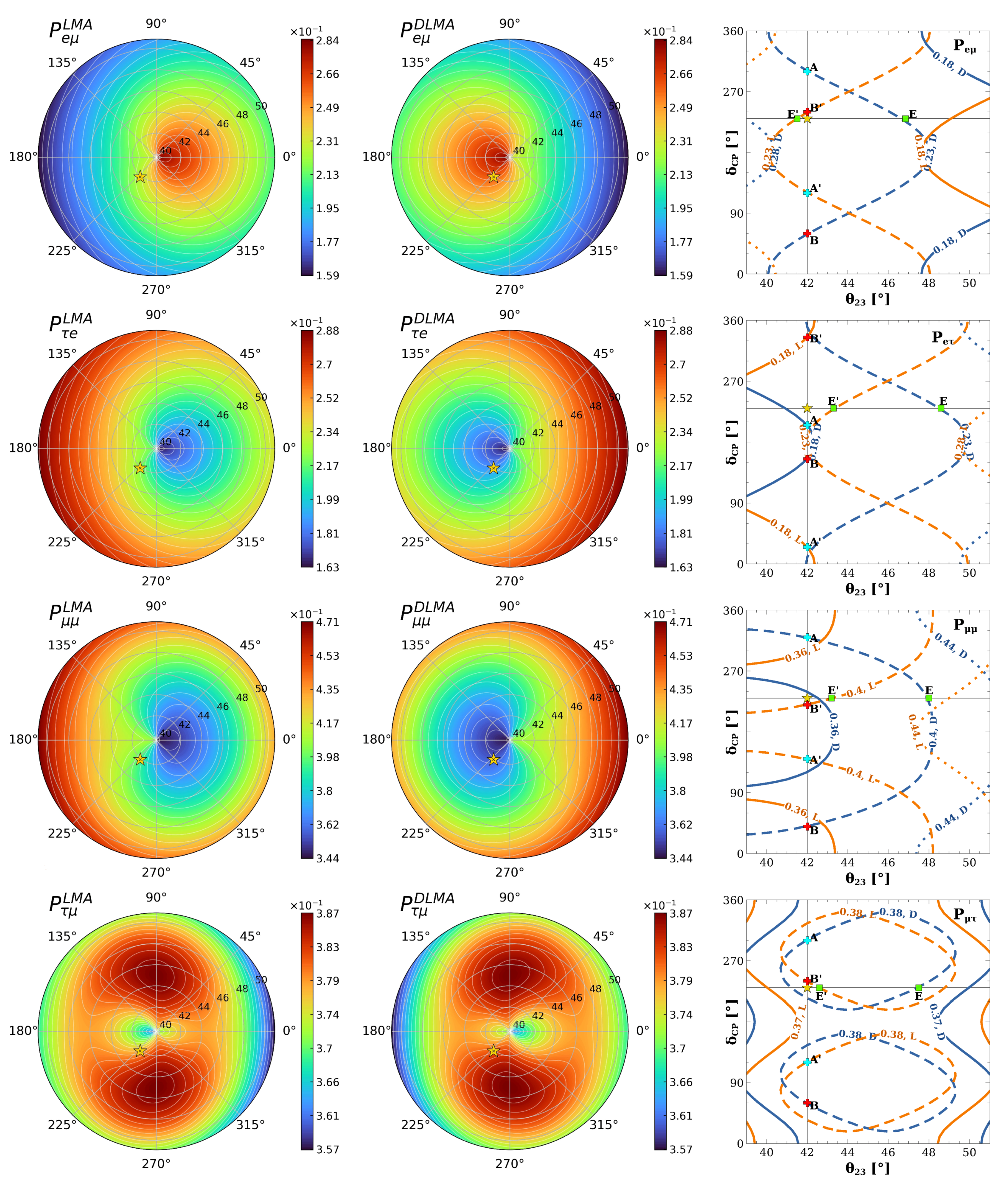
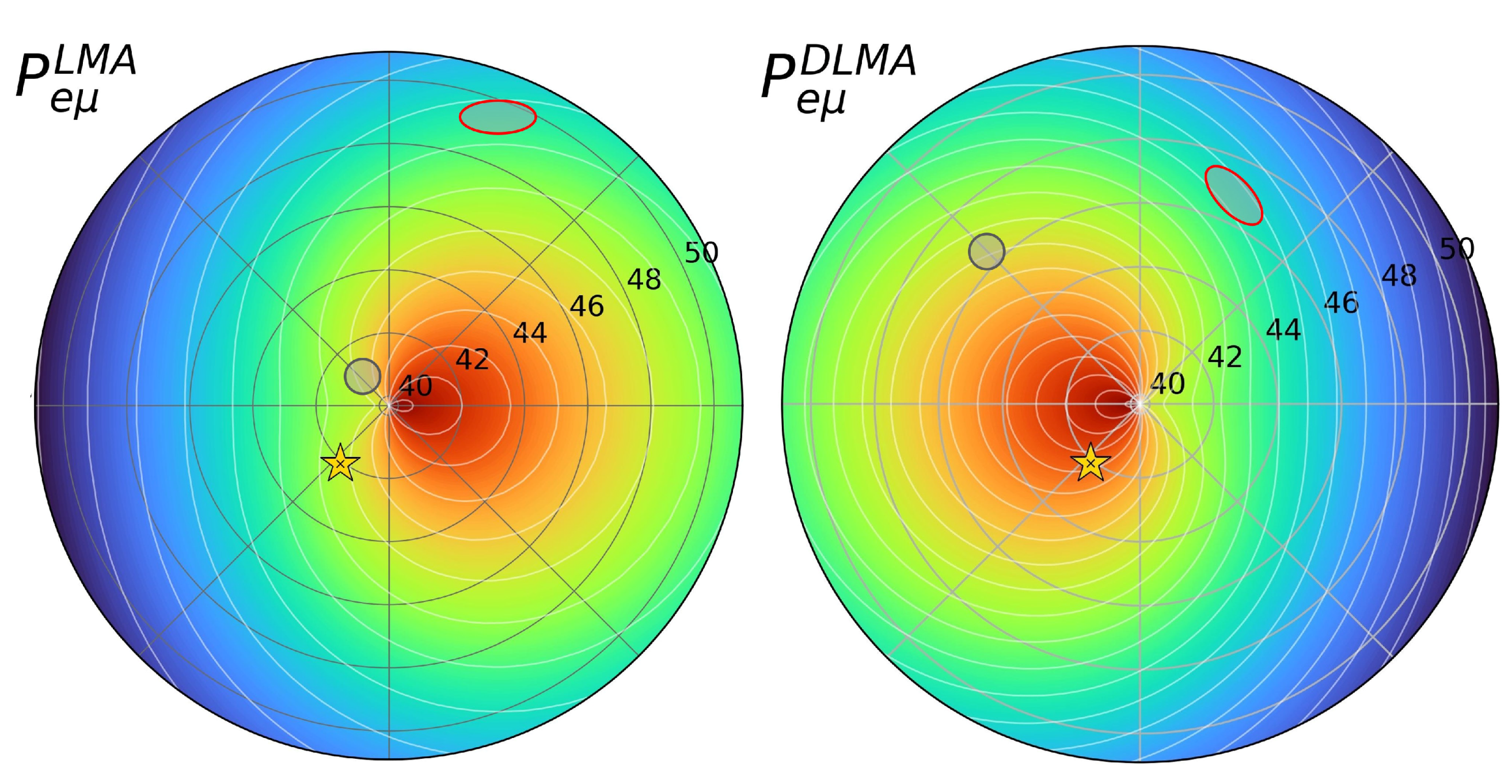
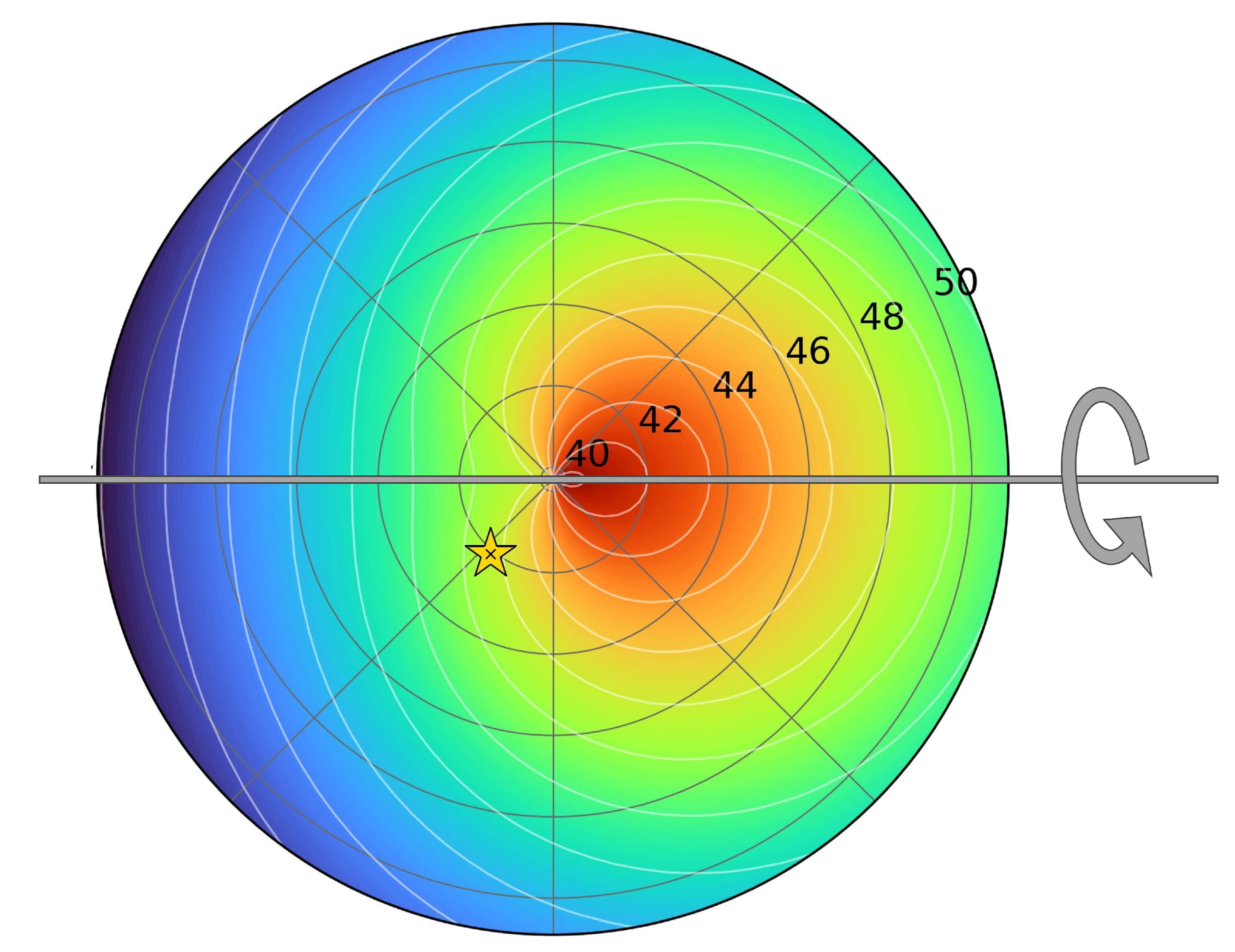
If we denote the flux of neutrinos of flavor $\alpha$ at the source by ${\varphi }_{\alpha }^0$ and the final oscillated flux at Earth by ${\varphi }_{\alpha }$, then the relation between ${\varphi }_{\alpha }^0$ and ${\varphi }_{\alpha }$ can be written as

$$\begin{array}{c}\hfill \left(\begin{array}{c}{\varphi }_e\\ {\varphi }_{\mu }\\ {\varphi }_{\tau }\end{array}\right)=\left(\begin{array}{ccc}{P}_{ee}& P_{\mu e}& P_{\tau e}\\ P_{e\mu }& P_{\mu \mu }& P_{\tau \mu }\\ P_{e\tau }& P_{\mu \tau }& P_{\tau \tau }\end{array}\right)\left(\begin{array}{c}{\varphi }_e^0\\ {\varphi }_{\mu }^0\\ {\varphi }_{\tau }^0\end{array}\right),\end{array}$$

(1)

where $P_{\alpha \beta }$ is the oscillation probability for ${\nu }_{\alpha }\to {\nu }_{\beta }$, with $\alpha$ and $\beta$ being e, $\mu$, and $\tau$. From Equation (1), we can understand that the probabilities $P_{\tau e}$, $P_{\tau \mu }$, and $P_{\tau \tau }$ do not enter in the calculation for the final fluxes, as ${\varphi }_{\tau }^0=0$ for all the three sources, i.e, the $\pi$ source, $\mu$ source, and n source. The final flux depends upon $P_{\mu e}$, $P_{\mu \mu }$, and $P_{\mu \tau }$ for the $\mu$ source (${\varphi }_e^0={\varphi }_{\tau }^0=0$), whereas the final flux depends only on $P_{ee}$, $P_{e\mu }$, and $P_{e\tau }$ for the n source (${\varphi }_{\mu }^0={\varphi }_{\tau }^0=0$). Therefore, when analyzing a particular source, it will be sufficient to look at the relevant probabilities to understand the numerical results.

For the energy and baselines related to IceCube, the probabilities can be calculated using the following formula:

$$\begin{array}{ccc}\hfill P_{\alpha \beta }& =& {\delta }_{\alpha \beta }-2\mathrm{Re}\sum _{i>j}{U}_{\alpha j}{U}_{\alpha i}^{*}{U}_{\beta j}^{*}{U}_{\beta i}\hfill \end{array}$$

(2)

$$\begin{array}{ccc}& =& \sum _{i=1}^3|U_{\alpha i}{|}^2{\left|U_{\beta i}\right|}^2\hfill \end{array}$$

(3)

where U is the PMNS matrix having the parameters ${\theta }_{12}$, ${\theta }_{13}$, ${\theta }_{23}$, and ${\delta }_{\mathrm{CP}}$. From the above equation, we see that for IceCube, $P_{\alpha \beta }=P_{\beta \alpha }$. It is easy to obtain the expressions for the different probabilities by expanding Equation (3):

$$\begin{array}{c}\begin{array}{c}\hfill P_{ee}={cos}^4{\theta }_{12}{cos}^4{\theta }_{13}+{sin}^4{\theta }_{12}{cos}^4{\theta }_{13}+{sin}^4{\theta }_{13}\end{array}\end{array}$$

(4)

$$\begin{array}{c}\begin{array}{cc}\hfill P_{e\mu }& =[\frac{1}{2}{sin}^{2}2{\theta }_{12}{cos}^2{\theta }_{23}+{sin}^2{\theta }_{13}{sin}^2{\theta }_{23}(2-\frac{1}{2}{sin}^{2}2{\theta }_{12})\hfill \\ & +\frac{1}{2}sin2{\theta }_{23}sin{\theta }_{13}sin2{\theta }_{12}cos2{\theta }_{12}cos{\delta }_{\mathrm{CP}}]{cos}^2{\theta }_{13}\hfill \end{array}\end{array}$$

(5)

$$\begin{array}{c}\begin{array}{cc}\hfill P_{e\tau }& =[\frac{1}{2}{sin}^{2}2{\theta }_{12}{sin}^2{\theta }_{23}+{sin}^2{\theta }_{13}{cos}^2{\theta }_{23}(2-\frac{1}{2}{sin}^{2}2{\theta }_{12})\hfill \\ & -\frac{1}{2}sin2{\theta }_{23}sin{\theta }_{13}sin2{\theta }_{12}cos2{\theta }_{12}cos{\delta }_{\mathrm{CP}}]{cos}^2{\theta }_{13}\hfill \end{array}\end{array}$$

(6)

$$\begin{array}{c}\begin{array}{cc}\hfill P_{\mu \mu }& =[{sin}^2{\theta }_{12}{cos}^2{\theta }_{23}+{cos}^2{\theta }_{12}{sin}^2{\theta }_{13}{sin}^2{\theta }_{23}+\hfill \\ & \frac{1}{2}sin2{\theta }_{12}sin2{\theta }_{23}sin{\theta }_{13}cos{\delta }_{\mathrm{CP}}{]}^2+{cos}^4{\theta }_{13}{sin}^4{\theta }_{23}\hfill \\ & +[{cos}^2{\theta }_{12}{cos}^2{\theta }_{23}+{sin}^2{\theta }_{12}{sin}^2{\theta }_{13}{sin}^2{\theta }_{23}-\hfill \\ & \frac{1}{2}sin2{\theta }_{12}sin2{\theta }_{23}sin{\theta }_{13}cos{\delta }_{\mathrm{CP}}{]}^2\hfill \end{array}\end{array}$$

(7)

$$\begin{array}{c}\begin{array}{cc}\hfill P_{\mu \tau }& =\frac{1}{2}cos{\delta }_{\mathrm{CP}}cos2{\theta }_{12}cos2{\theta }_{23}sin2{\theta }_{12}sin2{\theta }_{23}sin{\theta }_{13}\times \hfill \\ & (1+{sin}^2{\theta }_{13})+\frac{1}{4}{sin}^{2}2{\theta }_{23}(1-\frac{1}{2}{sin}^{2}2{\theta }_{12})(1+{sin}^4{\theta }_{13})\hfill \\ & \frac{1}{2}{sin}^{2}2{\theta }_{12}{sin}^2{\theta }_{13}(1-\frac{1}{2}{sin}^{2}2{\theta }_{23})\hfill \end{array}\end{array}$$

(8)

As $P_{\tau \tau }$ does not appear in the calculation of the final fluxes for the astrophysical sources, we omitted the expression for this probability. Here, we note that the probability expression $P_{ee}$ is independent of ${\theta }_{23}$ and ${\delta }_{\mathrm{CP}}$. This expression is also invariant under ${\theta }_{12}$ and ${90}^{\circ }-{\theta }_{12}$, i.e., ${\theta }_{12}^{\mathrm{LMA}}\to {\theta }_{12}^{DLMA}$.

In Figure 1, we plot the probabilities which are relevant for the IceCube energy and baselines, i.e., all the four probabilities except $P_{ee}$ and $P_{\tau \tau }$. In the left and middle columns, we present the polar plots of probabilities in ${\theta }_{23}$ and ${\delta }_{\mathrm{CP}}$ plane. The polar radius represents the ${\theta }_{23}$ axis, i.e., the minimum (maximum) radius corresponds to ${\theta }_{23}={40}^{\circ }({51}^{\circ }$), and the polar angle represents the ${\delta }_{\mathrm{CP}}$ axis. The different color shades correspond to different values of the probability, as shown in the columns next to the panels. The left column is for the LMA solution, and the middle is for the DLMA solution. Rows represent different probabilities written next to the panels. In the right column, we show the iso-probability curves in the ${\theta }_{23}$−${\delta }_{\mathrm{CP}}$ plane for both LMA and DLMA values of ${\theta }_{12}$. The orange curves are for LMA solution, and the blue curves are for DLMA solution. The values of the oscillation probabilities are written on the curves. In all panels, the current best-fit value of the ${\theta }_{23}$ and ${\delta }_{\mathrm{CP}}$ are marked by a star. We used the current best-fit values of ${\theta }_{12}$ and ${\theta }_{13}$ to generate this figure. These values are listed in

Table 1. The table depicts the best-fit values of all the parameters and their range of marginalization, which is taken from NuFit 5.1 [1]. The values of DLMA are evaluated as ${90}^{\circ }-{\theta }_{12}$(LMA).

Parameter	Best Fit	Marginalization Range
${\theta }_{12}$(LMA)	$33.4^{\circ }$	$31.{27}^{\circ }$:$35.{87}^{\circ }$
${\theta }_{12}$(DLMA)	$56.6^{\circ }$	$54.{13}^{\circ }$:$58.{73}^{\circ }$
${\theta }_{13}$	$8.{62}^{\circ }$	$8.{25}^{\circ }$:$8.{98}^{\circ }$
${\theta }_{23}$	$42.1^{\circ }$	${39}^{\circ }$:${51}^{\circ }$
${\delta }_{\mathrm{CP}}$	${230}^{\circ }$	$0^{\circ }$:${360}^{\circ }$

.

From the figure, the following observations can be made regarding the measurement of ${\theta }_{23}$, ${\delta }_{\mathrm{CP}}$, and the LMA and DLMA solution of ${\theta }_{12}$ in IceCube:

• For a given value of ${\theta }_{23}$, we notice a parameter degeneracy defined by $P_{\alpha \beta }({\theta }_{12}^{LMA},{\delta }_{\mathrm{CP}})=P_{\alpha \beta }({\theta }_{12}^{DLMA},{180}^{\circ }-{\delta }_{\mathrm{CP}})$. This can be observed from the panels in the left and the middle column in the following way. Imagine rotating the panels corresponding to the DLMA solution around the axis (perpendicular to the plane of the paper) passing through the center by ${180}^{\circ }$. These panels now look the same as the ones for the LMA solution (shown explicitly in the Appendix A). This transformation represents ${\delta }_{\mathrm{CP}}\to {180}^{\circ }-{\delta }_{\mathrm{CP}}$ degeneracy between the two solutions. This can also be seen by drawing an imaginary vertical line on panels in the right column. For example, this is shown by the vertical line at ${\theta }_{23}={42}^{\circ }$.
  From the right column of Figure 1, one can see that the probability for point A is the same as the probability in point $A^{\prime }$ and similar for B as $B^{\prime }$. And the points A and $A^{\prime }$ (also B and $B^{\prime }$) are separated by ${\delta }_{\mathrm{CP}}\to {180}^{\circ }-{\delta }_{\mathrm{CP}}$. We also see that points A($A^{\prime }$) (blue plus) and B($B^{\prime }$) (red plus) are degenerate with each other. We discuss this later. The origin of degeneracy discussed above, also known as Coloma–Schwetz symmetry, stems at the Hamiltonian level. In vacuum oscillations, the Hamiltonian of neutrino oscillation is invariant for the following transformation [9]:

  $$\begin{array}{ccc}\hfill \Delta m_{31}^2& \to & -\Delta m_{32}^2\hfill \end{array}$$

  (9)

  $$\begin{array}{ccc}\hfill sin{\theta }_{12}& \to & cos{\theta }_{12}\hfill \end{array}$$

  (10)

  $$\begin{array}{ccc}\hfill {\delta }_{\mathrm{CP}}& \to & {180}^{\circ }-{\delta }_{\mathrm{CP}}\hfill \end{array}$$

  (11)
  This can also be viewed from Equation (5) to Equation (8) in the following way. The difference between the probabilities due to the the LMA and DLMA solutions while keeping other parameters constant can be calculated as $\Delta P_{\alpha \beta }=P_{\alpha \beta }\left({\theta }_{12}\right)-P_{\alpha \beta }({90}^{\circ }-{\theta }_{12})$. Then, the differences are given as follows:

  $$\begin{array}{ccc}\hfill \Delta P_{e\mu }& =& sin2{\theta }_{12}cos2{\theta }_{12}sin{\theta }_{13}{cos}^2{\theta }_{13}sin2{\theta }_{23}cos{\delta }_{\mathrm{CP}}\hfill \end{array}$$

  (12)

  $$\begin{array}{ccc}\hfill \Delta P_{e\tau }& =& -sin2{\theta }_{12}cos2{\theta }_{12}sin{\theta }_{13}{cos}^2{\theta }_{13}sin2{\theta }_{23}cos{\delta }_{\mathrm{CP}}\hfill \end{array}$$

  (13)

  $$\begin{array}{ccc}\hfill \Delta P_{\mu \mu }& =& 2sin2{\theta }_{12}cos2{\theta }_{12}sin{\theta }_{13}{cos}^2{\theta }_{13}sin2{\theta }_{23}cos{\delta }_{\mathrm{CP}}({sin}^2{\theta }_{23}{sin}^2{\theta }_{13}-{cos}^2{\theta }_{23})\hfill \end{array}$$

  (14)

  $$\begin{array}{ccc}\hfill \Delta P_{\mu \tau }& =& sin2{\theta }_{12}cos2{\theta }_{12}sin{\theta }_{13}{cos}^2{\theta }_{13}sin2{\theta }_{23}cos{\delta }_{\mathrm{CP}}(1+{sin}^2{\theta }_{13})cos2{\theta }_{23}\hfill \end{array}$$

  (15)

  It can be observed that $\Delta P_{\alpha \beta }=0$ when ${\delta }_{\mathrm{CP}}={90}^{\circ }$ and ${270}^{\circ }$. We identify that the terms $sin2{\theta }_{23}$ and $cos{\delta }_{\mathrm{CP}}$ are the reason behind the degeneracies of LMA and DLMA solutions with ${\theta }_{23}$ and ${\delta }_{\mathrm{CP}}$. If we equate the probabilities for LMA and DLMA at fixed ${\theta }_{23}$, then the relation between different ${\delta }_{\mathrm{CP}}$ values for LMA and DLMA is given as

  $$cos{\delta }_{\mathrm{CP}}^{LMA}=-cos{\delta }_{\mathrm{CP}}^{DLMA}=cos[{180}^{\circ }-{\delta }_{\mathrm{CP}}^{DLMA}]$$

  (16)
  Therefore, from the IceCube experiment alone, it will not be possible to separate the LMA solution from the DLMA solution. However, if ${\delta }_{\mathrm{CP}}$ can be measured from a different experiment, then IceCube gives the opportunity to break the generalized mass-ordering degeneracy as the oscillation probabilities are independent of $\Delta m_{31}^2$ in IceCube.
• In these probabilities, there also exists a degeneracy between ${\theta }_{23}$ and the two solutions of ${\theta }_{12}$ for a given value of ${\delta }_{\mathrm{CP}}$. This can be viewed from the right column by drawing an imaginary horizontal line in the right panels. To show this, we drew a horizontal line at ${\delta }_{\mathrm{CP}}={230}^{\circ }$. This line intersects blue curves and orange curves having equal probabilities, showing the degeneracy between ${\theta }_{23}$ and the two solutions of ${\theta }_{12}$ for a given value of ${\delta }_{\mathrm{CP}}$. This degeneracy can also be seen on polar plots. Here, fixing the value of ${\delta }_{\mathrm{CP}}$ is equivalent to drawing a line that comes out of the center at a polar angle that is equal to the value of ${\delta }_{\mathrm{CP}}$. Next, we pick a certain shade of color, which corresponds to fixing a value of the probability. By reading the value of the radius where the line and this colored patch intersect, we obtain ${\theta }_{23}$, which does not necessarily have to be the same for the LMA and DLMA solutions (shown explicitly in the Appendix A). However, unlike the degeneracy mentioned in the earlier item, this degeneracy is not intrinsic.
  The degenerate values of ${\theta }_{23}$ corresponding to the LMA and DLMA solutions for a particular probability depend on the value of ${\delta }_{\mathrm{CP}}$. Let us show this explicitly in the case of $P_{e\mu }$. This degeneracy for $P_{e\mu }$ is defined by $P_{e\mu }({\theta }_{12}^{LMA},{\theta }_{23}^L)=P_{e\mu }({\theta }_{12}^{DLMA},{\theta }_{23}^D)$ which gives,

  $$\begin{array}{ccc}& & (sin{\theta }_{23}^L+sin{\theta }_{23}^D)\left\{-\frac{M_2}{2}cos{\delta }_{\mathrm{CP}}({sin}^2{\theta }_{23}^L-sin{\theta }_{23}^{L}sin{\theta }_{23}^D+{sin}^2{\theta }_{23}^D)+M_1(sin{\theta }_{23}^L-sin{\theta }_{23}^D)+M_{2}cos{\delta }_{\mathrm{CP}}\right\}=0\hfill \end{array}$$

  (17)
  This implies

  $$\begin{array}{ccc}& & (sin{\theta }_{23}^L+sin{\theta }_{23}^D)=0\mathrm{or}\left\{-\frac{M_2}{2}cos{\delta }_{\mathrm{CP}}({sin}^2{\theta }_{23}^L-sin{\theta }_{23}^{L}sin{\theta }_{23}^D+{sin}^2{\theta }_{23}^D)+M_1(sin{\theta }_{23}^L-sin{\theta }_{23}^D)+M_{2}cos{\delta }_{\mathrm{CP}}\right\}=0\hfill \end{array}$$

  (18)

  where $M_1={sin}^2{\theta }_{13}(2-\frac{1}{2}{sin}^{2}2{\theta }_{12})-\frac{1}{2}{sin}^{2}2{\theta }_{12}$ and $M_2=sin{\theta }_{13}sin2{\theta }_{12}cos2{\theta }_{12}$ are constants.
  The solution $(sin{\theta }_{23}^L+sin{\theta }_{23}^D)=0$ suggests that the degenerate solution is given by ${\theta }_{23}^L={360}^{\circ }-{\theta }_{23}^D$. But this cannot be observed in Figure 1, as ${360}^{\circ }-{\theta }_{23}^D$ do not lie in the range of ${39}^{\circ }-{51}^{\circ }$. For the other solution, with ${\delta }_{\mathrm{CP}}={90}^{\circ }$ and ${270}^{\circ }$, it gives simply $sin{\theta }_{23}^L-sin{\theta }_{23}^D=0$, i.e., ${\theta }_{23}^L={\theta }_{23}^D$, as seen Figure 1. In the case of other values of ${\delta }_{\mathrm{CP}}$, the angles ${\theta }_{23}^L$ and ${\theta }_{23}^D$ are connected by a quadratic equation, i.e., two degenerate solutions. For ${\delta }_{\mathrm{CP}}={230}^{\circ }$, ${\theta }_{23}^L=41.5^{\circ }$ and ${\theta }_{23}^D=46.{95}^{\circ }$ are degenerate solutions, which is consistent with the points E${}^{\prime }$ and E, respectively, in the top-right panel of Figure 1 corresponding to the $P_{e\mu }$ value of 0.23.
• One more degeneracy defined by ${\delta }_{\mathrm{CP}}\to -{\delta }_{\mathrm{CP}}$ is easily visible in left and middle columns. It can be seen from the probability expressions that are degenerate for $cos{\delta }_{\mathrm{CP}}=cos[-{\delta }_{\mathrm{CP}}]=cos[{360}^{\circ }-{\delta }_{\mathrm{CP}}]$. This degeneracy within each of the LMA and DLMA solutions can be seen if the plots are flipped around a horizontal line going through the center. Each plot looks the same if it is flipped around that line (shown explicitly in the Appendix A). As mentioned earlier, this degeneracy is the reason why points A ($A^{\prime }$) and B ($B^{\prime }$) in the right column are degenerate. This degeneracy arises from

  $$\begin{array}{cc}\hfill & \mathrm{Re}\sum _{i>j}{U}_{\alpha j}{U}_{\alpha i}^{*}{U}_{\beta j}^{*}{U}_{\beta i}\hfill \\ \hfill =& sin{\theta }_{13}{cos}^2{\theta }_{13}sin{\theta }_{12}cos{\theta }_{12}sin{\theta }_{23}cos{\theta }_{23}cos{\delta }_{\mathrm{CP}}\hfill \end{array}$$

  (19)
  (cf. Equation (2)), which is invariant under ${\delta }_{\mathrm{CP}}\to -{\delta }_{\mathrm{CP}}$ [27].

In the next section, we see how these degeneracies manifest in the analysis of the IceCube data.

3. Analysis and Results

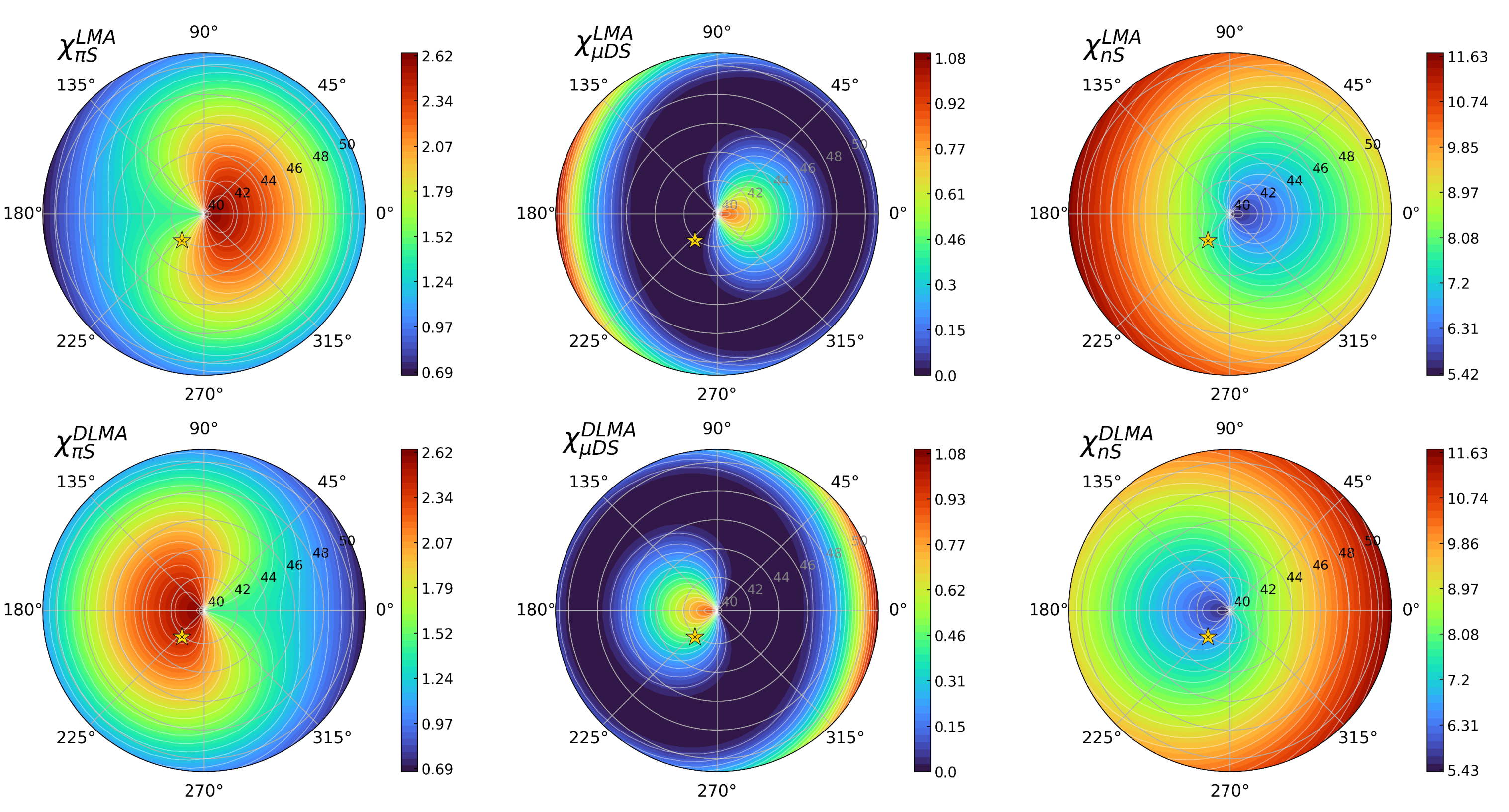
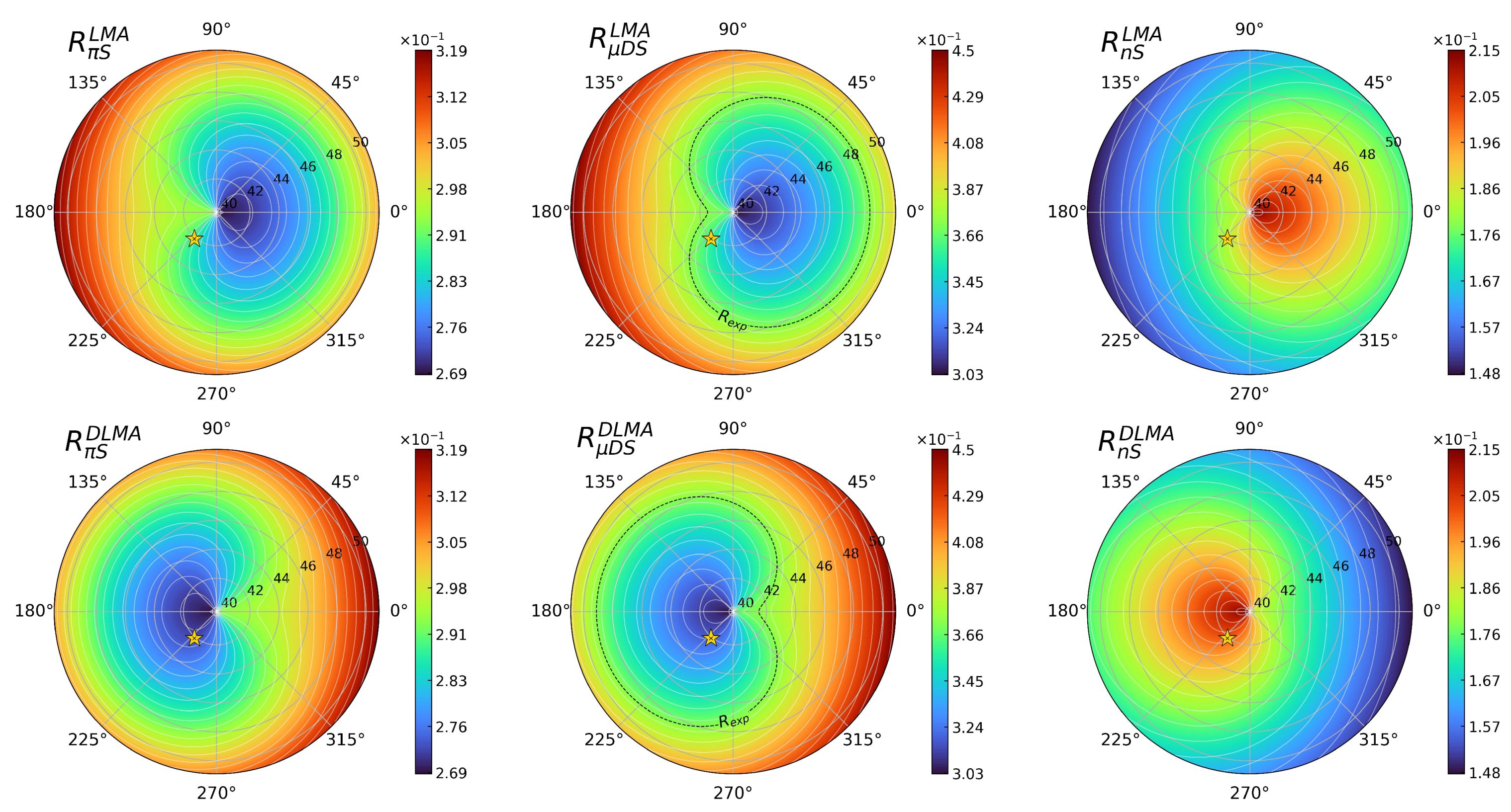
We analyzed the IceCube data in terms of track by shower ratio. The advantage of using this ratio is that one does not need the fluxes of the astrophysical neutrinos and the exact cross-sections to analyze the data of IceCube.

At IceCube, the muon event produces a track, whereas the electron and tau events produce a shower. In

Table 2. The observed events are categorized and presented. The left-most column indicates the event category, while the right-most column displays the total number of events observed in each category. The intermediate columns separate the events based on the reconstructed deposited energy, distinguishing between those with less than 60 TeV and those with greater than 60 TeV [28].

Category	$\mathit{E}<60$ TeV	$\mathit{E}>60$ TeV	Total
Total Events	42	60	102
Cascade	30	41	71
Track	10	17	27
Double Cascade	2	2	4

, we list the number of events from the 7.5 years of IceCube data. From these data, we calculate the experimental track by shower the ratio for the neutrinos having deposited energy greater than 60 TeV as [28]:

$$R_{exp}=\frac{17-1}{41+2}=\frac{16}{43}\approx 0.372.$$

(20)

In the above equation, we subtracted 1 from the numerator, because this is the number of events arising due to the atmospheric muons, and we treat this as a background. From the total number of tracks, we subtract the expected number of tracks produced by muons, which rounds up to 1. In the denominator, we added the events corresponding to cascade and double cascade to obtain the total number of shower events. Cascade events refer to a series of decays or interactions that produce a large number of secondary particles, and these events typically have a spherical topology. A double-cascade event occurs when an additional cascade event is created from showering particles, and the topology of these events resembles a distorted sphere.

To define a theoretical track by shower ratio, we refer to

Table 3. Expected events by category for best-fit parameters above 60 TeV are presented in tabular form. Each column represents the reconstructed event morphology, while each row corresponds to a specific particle. The top table displays the percentage of events expected in each morphology relative to the total number of events. The bottom table illustrates the percentage of events in each category for a specific morphology, where the percentages were calculated with respect to the total number of expected events for that particular morphology. When addressing background noise, the contribution of track events from muons will be taken into account. The percentages have been rounded to one decimal point [28].

Morphology	Cascade	Track	Double Cascade
Total	72.7%	23.4%	3.9%
${\nu }_e$	$56.7\%$	$9.8\%$	$21.1\%$
${\nu }_{\mu }$	$15.7\%$	$72.8\%$	$14.2\%$
${\nu }_{\tau }$	$27.6\%$	$10.5\%$	$64.7\%$
$\mu$	$0.0\%$	$6.9\%$	$0.0\%$

. This table shows the event morphology, i.e., the fraction of events from different neutrino flavors which can cause a track or a shower event at IceCube for deposited neutrino energy greater than 60 TeV. Using this information, one can define the theoretical track by shower ratio as

$$R=\frac{P_t{\sum }_{\alpha }{p}_t^{\alpha }{\varphi }_{\alpha }}{P_c{\sum }_{\alpha }{p}_c^{\alpha }{\varphi }_{\alpha }+P_{dc}{\sum }_{\alpha }{p}_{dc}^{\alpha }{\varphi }_{\alpha }}.$$

(21)

where $P_c/P_t/P_{dc}$ is the probability of obtaining a track/cascade/double cascade event at IceCube. These probabilities are given in the first row of Table 3. In the above equation, the probabilities for each neutrino flavor $\alpha$ leaving a track, cascade, or double cascade at IceCube is defined by $p_i^{\alpha }$, which are given in the second, third, and fourth row of the Table 3. The term ${\varphi }_{\alpha }$ is the flux of the oscillated neutrinos at Earth.

To compare these two $R_{exp}$ (cf. Equation (20)) and R (cf. Equation (21)), which we constructed above, we define a simple Gaussian ${\chi }^2$ in the following way:

$${\chi }^2={\left(\frac{R_{exp}-R({\theta }_{ij},{\delta }_{CP})}{{\sigma }_R}\right)}^2,$$

(22)

where ${\sigma }_R$ is given by

$${\sigma }_R=\sqrt{\frac{(1-R_{exp})R_{exp}}{N}},$$

(23)

with N being the total number of events [29]. As the total number of events is not very high, in our analysis, we did not consider any systematic uncertainty. We do not expect there to be a major impact of systematic uncertainties on our results.

In Figure 2, we plot the polar plots of this ${\chi }^2$ for the three different astrophysical sources in the ${\theta }_{23}$ and ${\delta }_{\mathrm{CP}}$ plane. In generating this plot, we minimized ${\theta }_{12}$ and ${\theta }_{13}$ over their $3\sigma$ allowed ranges, as listed in Table 1. In these panels, the different color shades correspond to different values of ${\chi }^2$, which are given in the columns next to the panels. The top row is for the LMA solution of ${\theta }_{12}$, whereas the bottom row is for the DLMA solution of ${\theta }_{12}$. In each row, the left panel is for $\pi$ source, the middle panel is for $\mu$ source, and the right panel is for n source. To understand the ${\chi }^2$ results, in Figure 3, we plot the same as in Figure 2 but for a theoretical track by shower ratio, i.e., R. This figure is generated using the best-fit values of ${\theta }_{12}$ and ${\theta }_{13}$. From Figure 2 and Figure 3, the following can be concluded:

• The variation in the color shading between the Figure 2 and Figure 3 is consistent. This shows the information of R is correctly reflected in the ${\chi }^2$ plots.
• The existence of degeneracy defined by ${\chi }^2/R({\theta }_{12}^{LMA},{\delta }_{\mathrm{CP}})={\chi }^2/R({\theta }_{12}^{DLMA},{180}^{\circ }-{\delta }_{\mathrm{CP}})$ for a given value of ${\theta }_{23}$ is clearly visible in Figure 2 and Figure 3. We can consider any point in these figures and take a ${180}^{\circ }$ transformation to obtain the degenerate solutions. The same arguments from the previous discussion also apply here.
• The degeneracy between ${\delta }_{\mathrm{CP}}\to -{\delta }_{\mathrm{CP}}$ for a given LMA/DLMA solution is also visible in Figure 2 and Figure 3.
• Degeneracy between ${\theta }_{23}$ and the two solutions of ${\theta }_{12}$ for a given value of ${\delta }_{\mathrm{CP}}$ is carried over from probabilities and is still present in Figure 2 and Figure 3.
• Among the three sources, the $\mu$ source is the most preferred source by the IceCube data as, for this source, we obtain a minimum ${\chi }^2$ value of 0 for both the LMA and DLMA solutions (middle column of Figure 2). From the panels, we see that the data do not prefer a particular value of ${\theta }_{23}$ and ${\delta }_{\mathrm{CP}}$, rather they are consistent with a region in the ${\theta }_{23}$–${\delta }_{\mathrm{CP}}$ plane. The best-fit regions of the ${\theta }_{23}$–${\delta }_{\mathrm{CP}}$ plane can be understood by looking at the middle column of Figure 3. In these panels, the value of $R_{exp}$ is drawn over R. This shows the values of ${\theta }_{23}$–${\delta }_{\mathrm{CP}}$ for which the prediction of the track by shower ratio matches exactly with the data. Note that though $R_{exp}$ in the middle column of Figure 3 is a curve, the best-fit region in the middle column of Figure 2 is not a curve; rather, it is a plane. The reason is two fold: (i) In Figure 2, we marginalized over the parameters ${\theta }_{13}$ and ${\theta }_{12}$. Because of this, there can be much more combinations of ${\theta }_{23}$ and ${\delta }_{\mathrm{CP}}$, which can give the exact value of $R_{exp}$ as compared with Figure 3, which is generated for a fixed value of ${\theta }_{13}$ and ${\theta }_{12}$. (ii) In polar plots, we do not have the precision to shade a region corresponding to exactly ${\chi }^2=0$. In these plots, ${\chi }^2=0$ is defined by a large set of very small numbers. This is why the best-fit region appears as a large black area. As we mentioned earlier, with the help of the ${\chi }^2$ plots, we can infer the true nature of ${\theta }_{12}$ given ${\delta }_{\mathrm{CP}}$ is measured from the other experiments. According to the current-best fit scenario, it can be said that IceCube data prefer the LMA solution of ${\theta }_{12}$ because, at this best-fit value (denoted by the star), we obtain the nonzero ${\chi }^2$ for the DLMA solution of ${\theta }_{12}$.
• The second most favored source according to the IceCube data is the $\pi$ source. For this source, the minimum ${\chi }^2$ is 0.7. As the minimum ${\chi }^2$ value is much less, one can say that the $\pi$ source and the $\mu$ source are almost equally favored. In this case, the best-fit region in the ${\theta }_{23}$–${\delta }_{\mathrm{CP}}$ plane is smaller than the $\mu$ source. For this source, the upper octant of ${\theta }_{23}$ is preferred for both the LMA and DLMA solutions of ${\theta }_{23}$. Regarding ${\delta }_{\mathrm{CP}}$, the best-fit value is around ${180}^{\circ }$ for the LMA solution of ${\theta }_{12}$, whereas for the DLMA solution of ${\theta }_{12}$, the best-fit value is around $0^{\circ }/{360}^{\circ }$. For this source, the current best-fit value (denoted by a star) is excluded at ${\chi }^2=1.7\left(2.4\right)$ for the LMA (DLMA) solution of ${\theta }_{12}$.
• The n source is excluded by IceCube at more than $2\sigma$ C.L., as the minimum ${\chi }^2$ in this case is 5.4. Similar to the $\pi$ source, in this case, the best-fit region in the ${\theta }_{23}$–${\delta }_{\mathrm{CP}}$ plane is smaller than the $\mu$ source. This source prefers the lower octant of ${\theta }_{23}$ for both the LMA and DLMA solutions of ${\theta }_{12}$. Regarding ${\delta }_{CP}$, the best-fit value is around ${180}^{\circ }$ for the DLMA solution of ${\theta }_{12}$, whereas for the LMA solution of ${\theta }_{12}$, the best-fit value is around $0^{\circ }/{360}^{\circ }$. For this source, the current best-fit value (denoted by a star) is excluded at ${\chi }^2=7.9\left(6.5\right)$ for the LMA (DLMA) solution of ${\theta }_{12}$.

4. Summary and Conclusions

In this paper, we studied the implications of measurement of ${\theta }_{23}$ and ${\delta }_{\mathrm{CP}}$ in IceCube data in the light of the DLMA solution of ${\theta }_{12}$. IceCube is an ongoing neutrino experiment at the south pole which studies the neutrinos coming from astrophysical sources. In the astrophysical sources, neutrinos are produced via three mechanisms: $\pi S$ process, $\mu DS$ process, and neutron decay. As the neutrinos coming from the astrophysical sources change their flavor during propagation, in principle, it is possible to measure the neutrino oscillation parameters by analyzing the IceCube data. Because of the large distance of the astrophysical sources and the high energy of the astrophysical neutrinos, the oscillatory terms in the neutrino oscillation probabilities get averaged out. As a result, the neutrino oscillation probabilities become independent of the mass square differences.

In our work, we first identified the oscillation probability channels which are responsible for the conversion of the neutrino fluxes for the three different sources mentioned above. Then, we identified the degeneracies in neutrino oscillation parameters that are relevant for IceCube. We showed that there exists an intrinsic degeneracy between the two solutions of ${\theta }_{12}$ and ${\delta }_{\mathrm{CP}}$. As this degeneracy stems at the Hamiltonian level, it is impossible for IceCube alone to measure ${\delta }_{\mathrm{CP}}$ and the true nature of ${\theta }_{12}$ at the same time. However, if ${\delta }_{\mathrm{CP}}$ can be measured from other experiments, it might be possible for IceCube to pinpoint the true nature of ${\theta }_{12}$. Apart from this, we also identified a degeneracy between ${\theta }_{23}$ and two possible solutions of ${\theta }_{12}$ for a fixed value of ${\delta }_{\mathrm{CP}}$. In addition, we also identified a degeneracy defined by ${\delta }_{\mathrm{CP}}\to {360}^{\circ }-{\delta }_{\mathrm{CP}}$ within the LMA and DLMA solution of ${\theta }_{12}$.

Taking the track by shower as an observable, we analyze the 7.5 years of IceCube data. Our results show that among the three sources, the IceCube data prefer the $\mu$ source. However, in this case, the data do not prefer a particular best-fit of ${\theta }_{23}$ and ${\delta }_{\mathrm{CP}}$; rather, the data are consistent with a large region in the ${\theta }_{23}$–${\delta }_{\mathrm{CP}}$ plane. After the $\mu$ source, the next most favorable source of astrophysical neutrinos according to the IceCube data is the $\pi$ source. However, as both the $\mu$ and $\pi$ sources are allowed within $1\sigma$, one can say that both sources are almost equally favored by IceCube. The n source is excluded at $2\sigma$ by IceCube. Unlike the $\mu$ source, the allowed region in the ${\theta }_{23}$–${\delta }_{\mathrm{CP}}$ plane is smaller for both the $\pi$ and n source. The $\pi$ (n) source prefers a higher (lower) octant for ${\theta }_{23}$ for both the LMA and DLMA solution of ${\theta }_{12}$. Regarding ${\delta }_{CP}$, the best-fit value is around ${180}^{\circ }$ ($0^{\circ }/{360}^{\circ }$) for the LMA (DLMA) solution of ${\theta }_{12}$, whereas for the DLMA (LMA) solution of ${\theta }_{12}$, the best-fit value is around $0^{\circ }/{360}^{\circ }$ (${180}^{\circ }$) for the $\pi$ (n) source. If we assume the current best-fit value of ${\theta }_{23}$ and ${\delta }_{\mathrm{CP}}$ to be true, then the $\mu$ and $\pi$ sources prefer the LMA solution of ${\theta }_{12}$, whereas the n source prefers the DLMA solution of ${\theta }_{12}$.

In conclusion, we can say that an analysis of IceCube data in terms of track by shower ratio can give important information regarding the measurement of ${\theta }_{23}$, ${\delta }_{\mathrm{CP}}$, and the true nature of ${\theta }_{12}$. However, we find that the current statistics of IceCube are too low to make any concrete statements regarding the above measurements.

References

1. Esteban, I.; González-García, M.C.; Maltoni, M.; Schwetz, T.; Zhou, A. The fate of hints: Updated global analysis of three-flavor neutrino oscillations. JHEP 2020, 9, 178. [Google Scholar] [CrossRef]
2. Abe, K. et al. [T2K Collaboration] Measurements of neutrino oscillation parameters from the T2K experiment using 3.6×10²¹ protons on target. arXiv 2023, arXiv:2303.03222. [Google Scholar]
3. Acero, M.A. et al. [NOvA Collaboration] Improved measurement of neutrino oscillation parameters by the NOvA experiment. Phys. Rev. D 2022, 106, 032004. [Google Scholar] [CrossRef]
4. De Gouvea, A.; Friedland, A.; Murayama, H. The Dark side of the solar neutrino parameter space. Phys. Lett. B 2000, 490, 125–130. [Google Scholar] [CrossRef]
5. Choubey, S.; Bandyopadhyay, A.; Goswami, S.; Roy, D.P. SNO and the solar neutrino problem. In Proceedings of the Conference on Physics Beyond the Standard Model: Beyond the Desert 02, Oulu, Finland, 2–7 June 2002; Volume 9, pp. 291–305. [Google Scholar]
6. Miranda, O.G.; Tórtola, M.A.; Valle, J.W. Are solar neutrino oscillations robust? JHEP 2006, 10, 8. [Google Scholar] [CrossRef]
7. Gonzalez-Garcia, M.C.; Maltoni, M. Determination of matter potential from global analysis of neutrino oscillation data. JHEP 2013, 9, 152. [Google Scholar] [CrossRef]
8. Dev, B.; Babu, K.S.; Denton, P.; Machado, P.; Argüelles, C.A.; Barrow, J.L.; Chatterjee, S.S.; Chen, M.C.; de Gouvêa, A.; Dutta, B.; et al. Neutrino Non-Standard Interactions: A Status Report. SciPost Phys. Proc 2019, 2, 001. [Google Scholar] [CrossRef]
9. Coloma, P.; Schwetz, T. Generalized mass ordering degeneracy in neutrino oscillation experiments. Phys. Rev. D 2016, 94, 055005. [Google Scholar] [CrossRef]
10. Choubey, S.; Pramanik, D. On Resolving the Dark LMA Solution at Neutrino Oscillation Experiments. JHEP 2020, 12, 133. [Google Scholar] [CrossRef]
11. Vishnudath, K.N.; Choubey, S.; Goswami, S. New sensitivity goal for neutrinoless double beta decay experiments. Phys. Rev. D 2019, 99, 095038. [Google Scholar]
12. Coloma, P.; Gonzalez-Garcia, M.C.; Maltoni, M.; Schwetz, T. COHERENT Enlightenment of the Neutrino Dark Side. Phys. Rev. D 2017, 96, 115007. [Google Scholar] [CrossRef]
13. Denton, P.B.; Farzan, Y.; Shoemaker, I.M. Testing large non-standard neutrino interactions with arbitrary mediator mass after COHERENT data. JHEP 2018, 7, 37. [Google Scholar] [CrossRef]
14. Coloma, P.; Denton, P.B.; Gonzalez-Garcia, M.C.; Maltoni, M.; Schwetz, T. Curtailing the Dark Side in Non-Standard Neutrino Interactions. JHEP 2017, 4, 116. [Google Scholar] [CrossRef]
15. Esteban, I.; Gonzalez-Garcia, M.C.; Maltoni, M.; Martinez-Soler, I.; Salvado, J. Updated constraints on non-standard interactions from global analysis of oscillation data. JHEP 2018, 8, 180. [Google Scholar] [CrossRef]
16. Coloma, P.; Gonzalez-Garcia, M.C.; Maltoni, M.; Pinheiro, J.P.; Urrea, S. Global constraints on non-standard neutrino interactions with quarks and electrons. arXiv 2023, arXiv:2305.07698. [Google Scholar] [CrossRef]
17. Aartsen, M.G. et al. [IceCube Collaboration] Evidence for High-Energy Extraterrestrial Neutrinos at the IceCube Detector. Science 2013, 342, 1242856. [Google Scholar]
18. Abbasi, R. et al. [IceCube Collaboration] Observation of high-energy neutrinos from the Galactic plane. Science 2013, 380, 6652. [Google Scholar]
19. Waxman, E.; Bahcall, J.N. High-energy neutrinos from astrophysical sources: An Upper bound. Phys. Rev. D 1999, 59, 023002. [Google Scholar] [CrossRef]
20. Hümmer, S.; Baerwald, P.; Winter, W. Neutrino Emission from Gamma-Ray Burst Fireballs, Revised. Phys. Rev. Lett. 2012, 108, 231101. [Google Scholar] [CrossRef] [PubMed]
21. Moharana, R.; Gupta, N. Tracing Cosmic accelerators with Decaying Neutrons. Phys. Rev. D 2010, 82, 023003. [Google Scholar] [CrossRef]
22. Athar, H.; Jeżabek, M.; Yasuda, O. Effects of neutrino mixing on high-energy cosmic neutrino flux. Phys. Rev. D 2000, 62, 103007. [Google Scholar] [CrossRef]
23. Rodejohann, W. Neutrino Mixing and Neutrino Telescopes. JCAP 2007, 1, 29. [Google Scholar] [CrossRef]
24. Meloni, D.; Ohlsson, T. Leptonic CP violation and mixing patterns at neutrino telescopes. Phys. Rev. D 2012, 86, 067701. [Google Scholar] [CrossRef]
25. Mena, O.; Palomares-Ruiz, S.; Vincent, A.C. Flavor Composition of the High-Energy Neutrino Events in IceCube. Phys. Rev. Lett. 2014, 113, 091103. [Google Scholar] [CrossRef]
26. Chatterjee, A.; Devi, M.M.; Ghosh, M.; Moharana, R.; Raut, S.K. Probing CP violation with the first three years of ultrahigh energy neutrinos from IceCube. Phys. Rev. D 2014, 90, 073003. [Google Scholar] [CrossRef]
27. Denton, P.B.; Parke, S.J. Simple and Precise Factorization of the Jarlskog Invariant for Neutrino Oscillations in Matter. Phys. Rev. D 2019, 100, 053004. [Google Scholar] [CrossRef]
28. Abbasi, R. et al. [IceCube Collaboration] The IceCube high-energy starting event sample: Description and flux characterization with 7.5 years of data. Phys. Rev. D 2021, 104, 022002. [Google Scholar] [CrossRef]
29. Lyons, L. Statistics for Nuclear and Particle Physicists; Cambridge University Press: Cambridge, UK, 1989. [Google Scholar]
Figure 1. The first two columns show contour plots of probabilities in δ C P θ 23 plane in polar projection. Best-fit values were taken for θ 12 and θ 13 . The polar radius represents θ 23 , and the polar angle represents δ CP . Values of probabilities are represented by colors shown next to the corresponding plot. The left column is for the LMA solution, and the middle is for the DLMA solution. The third column shows iso-probability curves for LMA (orange) and DLMA (blue) in conjunction. P e μ , P e τ , P μ μ m and P μ τ are shown in the panels of the first, second, third, and fourth row, respectively.
Universe 09 00380 g001
Figure 2. χ 2 polar contour plots in dependence of δ CP and θ 23 marginalized over θ 13 and θ 12 . The polar radius represents θ 23 , and the polar angle represents δ CP . Values of χ 2 , represented by colors, are shown next to the corresponding plots. The upper row shows calculations for the LMA solution and the lower row for the DLMA solution. Columns represent the pion source, muon source, and neutron source, respectively. Current best-fit value for θ 23 and δ CP is marked by a star at coordinates ( 42 . 1 , 230 ).
Universe 09 00380 g002
Figure 3. Track by shower ratio contour plots in dependence of δ CP and θ 23 . Best-fit values were taken for θ 12 and θ 13 . The polar radius represents θ 23 , and the polar angle represents δ CP . Values of χ 2 are represented by colors shown next to the corresponding plot. The upper row shows calculations for the LMA solution, and the lower row for the DLMA solution. Columns represent the pion source, muon source, and neutron source, respectively. The black dashed line represents the experimental value of the ratio measured at IceCube. The current best-fit value for θ 23 and δ CP and the corresponding value of the ratio for a given source are marked by a star at coordinates ( 42 . 1 , 230 ).
Universe 09 00380 g003