Abstract
Recently, the Einstein–Maxwell–scalar model with a non-minimal coupling between the scalar and Maxwell fields was explored. As a result, a new class of black hole solutions with scalar hair was discovered. By fixing the mass of a black hole and taking the maximum allowable charge, an extremal black hole was obtained. Interestingly, this extremal black hole not only possesses an event horizon with a non-zero surface area but also exhibits a non-zero Hawking temperature. This unique type of extremal black hole is referred to as a maximal warm hole (MWH). In this paper, we revisit this model and examine these black holes with highly excited state fields. We discovered that an excited state MWH solution can also be obtained under extremal conditions. We investigate the range of existence for excited states and analyze their relevant physical properties.
1. Introduction
Black holes, predicted by Einstein’s theory of general relativity, hold great significance in the field of astrophysics. Their existence has been confirmed through the detection of gravitational waves resulting from the merger of two black holes [1] and the remarkable imaging of black hole shadows by the Event Horizon Telescope (EHT) [2,3,4,5,6,7]. A defining characteristic of black holes is their possession of an event horizon, which acts as a boundary within the fabric of spacetime, effectively dividing it into distinct inner and outer regions. The event horizon behaves as a unidirectional membrane, permitting causal influences to traverse it solely in one direction [8]. Beyond the event horizon, certain black holes exhibit an additional feature known as a Cauchy horizon. Examples of black holes with Cauchy horizons include the Reissner–Nordstrom (RN) and Kerr black holes. The precise locations of the event and Cauchy horizons depend on the specific parameters characterizing the black hole, such as its mass, charge, or angular momentum. By satisfying specific relationships among these parameters, the event and Cauchy horizons coincide, giving rise to extremal black holes with the minimal achievable mass for a given charge and angular momentum. It is important to highlight that extremal black holes possess distinct causal structures that prevent them from being regarded as simple, continuous extrapolations of their non-extremal counterparts [9]. For example, extremal RN black holes possess a temperature of zero and exhibit a non-zero area for their degenerate horizon, yet their entropy vanishes. In contrast, extremal dilaton black holes, within the low-energy approximation model of string theory, feature a non-zero temperature and non-vanishing entropy, while their horizon is singular, resulting in a zero area [10]. Moreover, extensive research has been devoted to the study of extremal black holes with the aim of unraveling the origins of the Bekenstein–Hawking entropy. Numerous investigations have been conducted within this realm, exploring various aspects of extremal black holes [11,12,13,14,15,16].
Recently, a novel class of extremal black holes was discovered in the Einstein–Maxwell theory, non-minimally coupled to a complex, massive, gauged scalar field with coupling [17]. In the absence of the complex scalar field, the well-known Reissner–Nordstrom (RN) black hole solution can be obtained. However, if the non-minimal coupling term is absent, the existence of an RN black hole solution with complex scalar hair is precluded. Interestingly, when the electric charge of the black hole exceeds a certain threshold, the RN black hole becomes unstable and undergoes a phase transition, leading to the emergence of charged scalar hair due to the presence of the non-minimal coupling between the scalar and Maxwell fields. This behavior bears resemblance to the concept of holographic superconductivity in Anti–de Sitter (AdS) spacetime [18]. Notably, the authors have discovered that the charge of these new black holes with scalar hair can exceed their mass. Furthermore, under extremal conditions, these extremely hairy black holes possess a non-zero temperature, while the degenerate horizon retains a non-zero area without developing a singularity. This unique type of extremal black hole has been coined as a “maximal warm hole”. Additionally, the internal structures of these hairy black holes in the non-extremal case were investigated [19]. It has been observed that their behaviors align with the holographic superconducting model. Notably, no Cauchy horizon is present, and the internal scalar field exhibits Josephson-like oscillations.
Given that the scalar hair of these hairy black holes exists as a bound state, it is reasonable to expect the existence of excited states in addition to the ground state. Excited states are known to exhibit nodes along the radial direction, where the scalar field changes signs. Currently, there is significant research focused on the study of excited states of scalar fields in the presence of gravitational fields. For instance, there have been specific investigations into holographic superconductors with excited states [20,21,22], as well as works related to the study of boson stars [23,24]. In this paper, we revisit the model studied in [17] and obtain solutions for black holes with highly excited scalar fields. We find that under extremal conditions, an excited state MHW solution can also be obtained. Furthermore, we explore the range of existence of these excited state solutions and analyze their associated physical properties.
The paper is organized as follows. In Section 2, we review the Einstein–Maxwell–scalar model with non-minimal coupling between the scalar and Maxwell fields; we adopt spherically symmetric metrics, similar to the ansatz in [17]. In Section 3, we present the numerical results of excited hairy black holes and analyze their physical properties, especially the properties of excited MWH under extremal conditions. The conclusion and discussion are presented in the last section.
2. The Model
In this section, we review the Einstein–Maxwell–scalar model with non-minimal coupling between the scalar and Maxwell fields in [17], which can be written in the following form:
where the gauge covariant derivative is denoted by and is the gauge field strength tensor. The last term is the coupling term of the scalar and Maxwell fields with the coupling coefficient . When this last term is replaced with the cosmological constant in terms of the AdS length scale L, one could obtain the holographic superconductor model studied in [18].
Varying the action (1) with respect to the metric , the gauge field , and the scalar field , respectively, we obtain the following three equations of motion
where and are the energy–momentum tensors of the Maxwell and scalar fields, respectively,
If the complex, massive scalar field vanishes, the solution of the Einstein Equation (2), which can describe the asymptotically spherically black hole with charge, is the well-known RN black hole. When a non-trivial configuration of the complex scalar field exists, it is difficult to find out analytical solutions. Thus, we should solve the equations of motion (2) numerically to seek the scalar hairy black hole solutions.
In order to construct stationary solutions of a spherical BH with excited state scalar hair, we also adopt the spherical metric with similar coordinates to that in [17] within the following ansatz
where functions p and g are only functions of the radial coordinate r. For the Maxwell field, we only consider the case of the electrostatic field
where is the scalar potential. Based on the above metric and Maxwell’s ansatz, by calculating the r component of the Maxwell field equation, it can be determined that the phase of the static scalar field is constant; thus, the phase of the complex scalar could vanish by choosing the gauge. For convenience, we can take the scalar field as a real scalar in a similar way to the holographic superconductor.
Taking the above ansatz into Equation (2), we can obtain the second-order differential equations as follows:
The above equation is a set of coupled differential equations; we choose to use numerical methods instead of seeking analytical solutions. At the boundary , the asymptotic behaviors of the functions take the following forms
Here, the constant is the electrostatic potential at infinity. At the event horizon of the hairy black hole solution, we require
One additional clarification to note here is that for the equations of motion (8) involving two second-order ordinary differential equations and two first-order ordinary differential equations, it is customary that each second-order equation requires two boundary conditions, while each first-order equation requires one boundary condition. Therefore, the total number of boundary conditions needed should be . This means that when solving the boundary value problem associated with these equations, six boundary conditions need to be provided to ensure a unique solution. These boundary conditions can include values or constraints at the horizon, values or constraints at infinity, first-order derivatives, or other specified conditions. Ensuring the proper setup and fulfillment of these boundary conditions is crucial for obtaining a solution to the motion equations. We chose boundary conditions (9) and (10) to solve the motion equations and found that they yield good results in practical applications; thus, they are valid choices.
The ADM mass M and electrical charge Q in a black hole with scalar hair are the key quantities that we are interested in, which are encoded in the asymptotic expansion of metric components and
Before solving these equations numerically, we can know that there is a special trivial solution to the above equations. That is, when the scalar field is zero, there is a spherically symmetric RN black hole solution. As the coupling constant is larger than the critical value , the condensation of scalar hair begins to appear. We will study these properties numerically in the next section.
3. Numerical Results
In this section, we will solve the above coupled Equation (8) with boundary conditions (9) and (10) numerically. For convenience, we will change the radial coordinate r to a new radial coordinate . Thus, the boundaries of the computed region are fixed at and , respectively. In addition, we use a common pseudo-spectral collocation method to solve the nonlinear ordinary differential equations [25], employing a Newton–Raphson technique, and all functions are expressed as a series of Chebyshev polynomials in z. The number of typical grid points ranges between 60 and 100 in the integration region , and the relative error of the numerical solutions in our paper is estimated to be below .
Considering the characteristics of the Newton–Raphson method, we need an appropriate initial value of the unknown functions to ensure that the iteration can converge to the correct solutions. To numerically obtain the ground state solution, one could use the profile of a constant as an initial guess for the function . Meanwhile, for the n-th excited state case, one needs to choose an initial guess with n nodes for the function .
3.1. Critical Analysis of Scalar Field Stability
Before fully numerically solving the above set of ordinary differential equations, we can first analyze whether the solution we constructed is stable before the formation of scalar field condensation. Thus, we adopt a method similar to that in [26]. The method is divided into two steps: (1) Solve the Einstein and Maxwell equations to obtain an RN black hole as the background of the spacetime. (2) Solve the linear scalar field equation in the RN spacetime background. Thus, one could recast Equation (2c) to take the following appealing form
This linear equation can be viewed as an eigenvalue equation with respect to the scalar field , with being the eigenvalue. It is well known that the ground state scalar hair exhibits no nodes. In other words, along the radial direction r, the value of the scalar field remains constant with the same sign. Meanwhile, the excited states could have some nodes along the radial direction, where the value of the scalar field could change the sign. When the charge q and mass m are fixed, we can obtain a series of eigenfunctions corresponding to different values of by numerical methods. In addition to the zero-mode of corresponding to the ground state solution of the hairy black hole, non-zero modes of corresponding to excited hairy black holes exist. It is shown here that the different values of are critical values, such that below these values, the scalar field vanishes and the solution is the simple Reissner–Nordstrom metric. Above these values, the Reissner–Nordstrom solution becomes unstable and develops scalar hair, encompassing both ground and excited states.
In Figure 1, we show the critical value of where scalar field condensation can occur for a black hole with a fixed mass and , where three curves are depicted to represent the ground state (in black), first excited state (in red), and second excited state (in blue). In the upper panels, by varying the value of , one can obtain different critical values corresponding to black hole masses M with the fixed . One can see that with a fixed event horizon radius, as the black hole mass increases, the value of decreases, indicating that the scalar field is more likely to condense in the case of a large mass black hole. In order to obtain hairy black holes with scalar hair in excited states, larger values of the critical values are necessary. Meanwhile, in the lower panels, by varying the value of , one can obtain different critical values with a fixed value of . It is observed that, under the condition of a fixed , as the black hole mass increases, the value of also increases. This behavior is different from that shown in the upper plots. In comparison to the ground state solution, it was observed that for the coupling constant exceeding the critical value , the condensation of scalar hair emerges, which can be considered as the ground state solution. By further increasing the coupling constant to a new critical value, a novel branch of solutions with a radial node begins to develop, representing the first excited state solution. As continues to increase towards higher values, a sequence of excited states of the black hole with scalar hair can be obtained. Having determined the critical values , one can then solve the coupled Einstein–Maxwell–scalar equations to obtain the solutions for the case of the above , corresponding to the existence of hairy black holes.
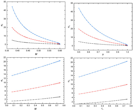
Figure 1.
The dependence of the critical value on the mass M of the RN black hole with . The black, red, and blue lines stand for the ground, first, and second excited states, respectively. Upper: Varying the value of with the fixed . Lower: Varying the value of with the fixed value of .
3.2. Numerical Hairy Black Hole Solution
In this subsection, we present our numerical solutions. First of all, in Figure 2, we present the configuration of the hairy black hole, in which the three colors, black, red, and blue, represent the ground state, the first excited state, and the second excited state, respectively. The distribution of the function of is shown in the lower left panel, which reveals one and two intersections on the x-axis of the first and second excitations, respectively. These intersections are a consequence of the excited state of the matter field, which causes the distribution of matter to no longer decrease monotonically from the center as in the ground state. As a result, the metric function p is also affected and may no longer be monotonic.

Figure 2.
The configuration of the hairy black hole solutions with , , and . The black, red, and blue lines stand for the ground, first, and second excited states, respectively.
In Figure 3, we present the relationship between the mass and the charge-mass difference of the hairy black holes with and . In the first row, we present the curves illustrating the relationships between various values of . The left panel corresponds to the ground state, the middle panel represents the first excited state, and the right panel corresponds to the second excited state. The red and black dashed lines are composed of the two endpoints of curves with different values of , meanwhile, the blue dashed line represents the maximal warm hole with . When is small, the difference between mass and charge can be positive or negative. As increases, the charge gradually increases, and the curve shifts upward as a whole. When is large, the charge can exceed the black hole mass. The blue dashed line corresponds to the extremal case of , which is the maximal warm hole. We can see that although the difference between charge and mass decreases as the black hole mass decreases, the black hole charge is always greater than its mass. To compare the difference between the ground and excited states more clearly, we plotted the cases of critical and MWH solutions in the two plots of the second row. Black, red, and blue represent the ground state, the first excited state, and the second excited state, respectively. We can observe that when the condensation of the scalar field occurs, the difference between the charge and mass of the black holes decreases as we transition from the ground state to the excited state. Moreover, the solutions of MWH with excited states have a larger charge compared to the solutions with the ground state. In particular, it can be seen that when the mass of the black hole is sufficiently large, the MWH solution will degenerate into an extremely hairless black hole, which is also known as the extremal RN black hole.
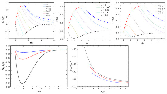
Figure 3.
The phase diagram of solutions with and . The first row of subplots corresponds to the ground state, first excited state, and the second excited state, respectively, with different values of . In the second row, the left and right panels represent the critical hairy black hole solutions and maximal warm holes, respectively, with the ground state denoted as black lines, the first excited state as red lines, and the second excited state as blue lines.
To gain a clearer understanding of the properties of the maximal warm holes, we present in Figure 4 the dependence between the black hole entropy S, temperature T, and on the mass for the case of . The black, red, and blue represent the ground state, the first excited state, and the second excited state, respectively. From the left plot, we can see that the entropy of the black hole monotonically increases with the black hole mass. Additionally, for the same entropy, excited states of maximal warm holes have larger masses. Considering that entropy is proportional to the square of the radius, black holes with the same event horizon radius but in an excited state have larger masses than the ground state of the maximal warm holes. From the middle panel, we can observe that the temperature of maximal warm holes initially increases with mass until it reaches a maximum value. After reaching the maximum, the temperature decreases monotonically with increasing mass. By comparing the maximum temperature values for the ground state and excited states, we can see that the maximum temperature decreases from ground to excited states. Furthermore, for the maximal warm holes with the same mass, the temperature of excited states decreases as the excited state increases. The right plot shows the variation of with mass. We can observe that as the mass increases, the starts increasing from its minimum non-zero value. The minimum value of each excited state is larger than the ground state.

Figure 4.
Physical properties of the maximal warm holes with , and . The three panels show the dependence between the entropy S, temperature T, and on the black hole mass M for the case of .
4. Conclusions
In this paper, we revisited the Einstein–Maxwell–scalar model with non-minimal coupling between the scalar and Maxwell fields and we numerically investigated the solutions of black holes with scalar hair. In addition to the ground state solution, we constructed numerical solutions for excited states, including the first and second excited states. Comparing these solutions with the ground state, we observed that when the coupling constant exceeds a critical value , the condensation of scalar hair appears, representing the ground state solution. As we further increase the coupling constant to another critical value, a new branch of solutions with a node in the radial direction emerges, corresponding to the first excited state solution. By increasing to higher values, we obtain a series of excited states for the black holes with scalar hair.
To determine the critical value , we treated the linear scalar field equation as an eigenvalue equation with respect to the scalar field , where serves as the eigenvalue. By comparing the differences between the ground and excited states, we found that as the scalar field condenses, the disparity between the charge and mass of the black holes decreases from the ground state to the excited state. Furthermore, when considering the extreme case, we also discovered the existence of maximal warm holes in the excited states. Compared to the maximal warm hole in the ground state, the maximal warm hole in the excited state exhibits a smaller charge-mass difference under the same black hole mass condition, along with lower Hawking temperature and black hole entropy.
There are several interesting extensions of our work. Firstly, we can introduce new non-minimal coupling terms, such as non-minimal coupling between the scalar field and Ricci curvature, to replace the current non-minimal coupling between the scalar and Maxwell fields. Secondly, we can replace the scalar field with a massive vector field, such as the complex Proca field studied in [27], to explore the possibility of Proca field condensation and generate black holes with Proca hair. Finally, in this paper, we only consider the existence and physical properties of the stationary solutions for excited states of hairy black holes. However, it is known that the usual excited states are kinetically unstable compared to the ground state. Therefore, our future work will focus on studying the dynamic stability properties of maximal warm holes.
Author Contributions
Conceptualization, Y.-Q.W.; methodology, Y.-Q.W.; software, Y.Y.; validation, Y.-Q.W.; formal analysis, Y.-Q.W.; investigation, Y.-Q.W.; writing—original draft preparation, Y.-Q.W.; writing—review and editing, Y.-Q.W.; visualization, Y.Y.; supervision, Y.-Q.W.; project administration, Y.-Q.W. All authors have read and agreed to the published version of the manuscript.
Funding
This research received no external funding.
Data Availability Statement
No new data were created or analyzed in this study.
Acknowledgments
Y.Y. is supported by the introduction of the talent research project of Northwest Minzu University (no. xbmuyjrc2020030). Y.Q.W is supported by the National Key Research and Development Program of China (grant no. 2020yfc2201503) and the National Natural Science Foundation of China (grant no. 12275110 and 12247101).
Conflicts of Interest
The authors declare no conflict of interest.
References
- Abbott, B.P. et al. [LIGO Scientific and Virgo] Observation of Gravitational Waves from a Binary Black Hole Merger. Phys. Rev. Lett. 2016, 116, 061102. [Google Scholar] [CrossRef] [PubMed]
- Akiyama, K. et al. [Event Horizon Telescope] First M87 Event Horizon Telescope Results. I. The Shadow of the Supermassive Black Hole. Astrophys. J. Lett. 2019, 875, L1. [Google Scholar]
- Akiyama, K. et al. [Event Horizon Telescope] First M87 Event Horizon Telescope Results. II. Array and Instrumentation. Astrophys. J. Lett. 2019, 875, L2. [Google Scholar]
- Akiyama, K. et al. [Event Horizon Telescope] First M87 Event Horizon Telescope Results. III. Data Processing and Calibration. Astrophys. J. Lett. 2019, 875, L3. [Google Scholar]
- Akiyama, K. et al. [Event Horizon Telescope] First M87 Event Horizon Telescope Results. IV. Imaging the Central Supermassive Black Hole. Astrophys. J. Lett. 2019, 875, L4. [Google Scholar]
- Akiyama, K. et al. [Event Horizon Telescope] First M87 Event Horizon Telescope Results. V. Physical Origin of the Asymmetric Ring. Astrophys. J. Lett. 2019, 875, L5. [Google Scholar]
- Akiyama, K. et al. [Event Horizon Telescope] First M87 Event Horizon Telescope Results. VI. The Shadow and Mass of the Central Black Hole. Astrophys. J. Lett. 2019, 875, L6. [Google Scholar]
- Misner, C.W.; Thorne, K.S.; Wheeler, J.A. Gravitation; WH Freeman and Company Limited: New York, NY, USA, 1973; ISBN 978-0-7167-0344-0, 978-0-691-17779-3. [Google Scholar]
- Hawking, S.W.; Horowitz, G.T.; Ross, S.F. Entropy, Area, and black hole pairs. Phys. Rev. D 1995, 51, 4302–4314. [Google Scholar] [CrossRef]
- Garfinkle, D.; Horowitz, G.T.; Strominger, A. Charged black holes in string theory. Phys. Rev. D 1991, 43, 3140, Erratum in Phys. Rev. D 1992, 45, 3888. [Google Scholar] [CrossRef]
- Strominger, A.; Vafa, C. Microscopic origin of the Bekenstein-Hawking entropy. Phys. Lett. B 1996, 379, 99–104. [Google Scholar] [CrossRef]
- Callan, C.G.; Maldacena, J.M.; Peet, A.W. Extremal black holes as fundamental strings. Nucl. Phys. B 1996, 475, 645–678. [Google Scholar] [CrossRef]
- Horowitz, G.T.; Strominger, A. Counting states of near extremal black holes. Phys. Rev. Lett. 1996, 77, 2368–2371. [Google Scholar] [CrossRef] [PubMed]
- Teitelboim, C. Action and entropy of extreme and nonextreme black holes. Phys. Rev. D 1995, 51, 4315, Erratum in Phys. Rev. D 1995, 52, 6201. [Google Scholar] [CrossRef] [PubMed]
- Ghosh, A.; Mitra, P. Understanding the area proposal for extremal black hole entropy. Phys. Rev. Lett. 1997, 78, 1858–1860. [Google Scholar] [CrossRef]
- Hod, S. Evidence for a null entropy of extremal black holes. Phys. Rev. D 2000, 61, 084018. [Google Scholar] [CrossRef]
- Dias, O.J.C.; Horowitz, G.T.; Santos, J.E. Extremal black holes that are not extremal: Maximal warm holes. JHEP 2022, 1, 64. [Google Scholar] [CrossRef]
- Hartnoll, S.A.; Herzog, C.P.; Horowitz, G.T. Building a Holographic Superconductor. Phys. Rev. Lett. 2008, 101, 031601. [Google Scholar] [CrossRef]
- Dias, O.J.C.; Horowitz, G.T.; Santos, J.E. Inside an asymptotically flat hairy black hole. JHEP 2021, 12, 179. [Google Scholar] [CrossRef]
- Wang, Y.Q.; Hu, T.T.; Liu, Y.X.; Yang, J.; Zhao, L. Excited states of holographic superconductors. JHEP 2020, 6, 13. [Google Scholar] [CrossRef]
- Qiao, X.; Wang, D.; OuYang, L.; Wang, M.; Pan, Q.; Jing, J. An analytic study on the excited states of holographic superconductors. Phys. Lett. B 2020, 811, 135864. [Google Scholar] [CrossRef]
- Wang, D.; Du, X.; Pan, Q.; Jing, J. Holographic p-Wave Superconductor with Excited States in 4D Einstein–Gauss–Bonnet Gravity. Universe 2023, 9, 104. [Google Scholar] [CrossRef]
- Bernal, A.; Barranco, J.; Alic, D.; Palenzuela, C. Multi-state Boson Stars. Phys. Rev. D 2010, 81, 044031. [Google Scholar] [CrossRef]
- Wang, Y.Q.; Liu, Y.X.; Wei, S.W. Excited Kerr black holes with scalar hair. Phys. Rev. D 2019, 99, 064036. [Google Scholar] [CrossRef]
- Trefethen, L.N. Spectral Methods in MATLAB; SIAM: Philadelphia, PA, USA, 2000. [Google Scholar]
- Horowitz, G.T.; Santos, J.E. General Relativity and the Cuprates. JHEP 2013, 6, 87. [Google Scholar] [CrossRef]
- Brito, R.; Cardoso, V.; Herdeiro, C.A.R.; Radu, E. Proca stars: Gravitating Bose–Einstein condensates of massive spin 1 particles. Phys. Lett. B 2016, 752, 291–295. [Google Scholar] [CrossRef]


Disclaimer/Publisher’s Note: The statements, opinions and data contained in all publications are solely those of the individual author(s) and contributor(s) and not of MDPI and/or the editor(s). MDPI and/or the editor(s) disclaim responsibility for any injury to people or property resulting from any ideas, methods, instructions or products referred to in the content. |
© 2023 by the authors. Licensee MDPI, Basel, Switzerland. This article is an open access article distributed under the terms and conditions of the Creative Commons Attribution (CC BY) license (https://creativecommons.org/licenses/by/4.0/).