Abstract
Oort constants and local kinematics are vital parameters with which to study the structure and dynamics of the Milky Way. When GCNS was published, it provided a clean sample of stars in the solar vicinity, which gives us an ideal tool with which to determine these parameters. Our aim was to calculate the reliable Oort constants with GCNS. We determined the Oort constants using the GCNS from Gaia EDR3 with . The proper motions and radial velocities were fitted with a maximum likelihood model. The uncertainties were obtained with an MCMC method. The sample was carefully selected to obtain a reliable result. The result yields the Oort constants , , , and . The non-zero C and K imply that the local disc is in a non-asymmetric potential. With the Oort constants, we derived the local angular velocity . The solar motion (, , ) was calculated as (, , ) .
1. Introduction
Calculating the rotation curve of the Milky Way poses a challenging task because our observations are made from within the solar system. However, the properties of the galactic disk can be inferred by carefully examining the kinematics of stars in our solar vicinity. These kinematic parameters, referred to as Oort constants, are vital in the study of the structure and dynamics of the Milky Way. These constants were first derived and determined by [1], marking a major milestone in our understanding of the Milky Way. To compute the Oort constants, Oort utilized the first Taylor expansion of the stellar velocity in the solar vicinity. This method necessitates that the stars be located in close proximity to the Sun. Consequently, the kinematics of stars in the solar vicinity play a crucial role in determining these parameters. They provide us with a unique insight into the galactic disk’s intricate structure and dynamics. In this context, the Gaia Catalog of Nearby Stars (GCNS, [2]), released in tandem with the Gaia Early Data Release 3 (EDR3) by the Gaia mission, is of immense value. The GCNS catalogues stars located within a 100 radius of the Sun, providing us with a rich data set of stars in our immediate solar vicinity. This comprehensive dataset furnishes an optimal platform for the precise measurement of the Oort constants, thereby furthering our understanding of the rotation and structure of the Milky Way.
Typically, Oort constants are determined using the proper motions and radial velocities of local stars in the vicinity of the Sun. Throughout history, many attempts have been made to calculate Oort constants. A commonly used set of values for the Oort constants is , , which were derived using the HIPPRACOS proper motions of Cepheids [3]. Since the release of the Gaia [4] catalog, many efforts have been made to determine the Oort constants using Gaia data. Bovy [5] determined the Oort constants to be , , , and using proper motions from Gaia data release 1 (DR1) Tycho-Gaia Astrometric Solution (TGAS) main-sequence stars. Li et al. [6] found the Oort constants to be , , , and with the publication of Gaia Data Release 2 (DR2). Wang et al. [7] calculated the Oort constants using A-type stars, resulting in values of , , , and . While there are slight differences in the results of these calculations, they all indicate that C and K are non-zero values, revealing that the Milky Way is not axisymmetric.
Gaia, developed by the European Space Agency (ESA), is the successor to the astrometric satellite HIPPRACOS. Its mission [4] began in 2006, and the spacecraft was launched in December 2013. One of Gaia’s primary scientific goals is to map and understand the structure and dynamics of the Milky Way. The space telescope measures the three-dimensional spatial and velocity distribution of targets with unparalleled accuracy. ESA has released three Gaia data releases, which have significantly improved our understanding of the structure and dynamics of the Milky Way. The third intermediate Gaia data release (Gaia EDR3), was released on 3 December 2020 and Gaia DR3 was released on 13 June 2022. The astrometric parameters and broad-band photometry have been updated between Gaia DR2 and (E)DR3. Gaia (E)DR3 lists about 1.8 billion sources, including 1.46 billion sources with parallaxes, proper motions, and the ( − ) color. The Gaia (E)DR3 has improved parallax precision by 30% compared to Gaia DR2, and proper motion precision has been doubled. These unprecedented, high-precision astrometry data provide a new sample for calculating the Oort constants.
Along with the Gaia EDR3, the GCNS is also published, which is a highly curated collection of celestial objects located within 100 of the Sun, derived from data obtained from Gaia EDR3. The catalogue is a comprehensive, well-characterized record, with each object having an inferred distance probability density function calculated using parallaxes and a single distance prior. GCNS is truly an astronomical landmark, representing a substantial improvement over previous nearby star censuses. With an impressive 331,312 entries, it marks a tenfold increase in data volume compared to the most complete pre-Gaia mission census. Moreover, Gaia EDR3 is significantly cleaner than its predecessor, Gaia DR2, and yet GCNS contains a few percent of real objects that are not included in Gaia EDR3. GCNS achieves an overall completeness of more than 95% for objects up to M8 spectral type within 100 . The information contained within the GCNS extends beyond mere celestial coordinates. For all sources, the all-sky maps at HEALpix level 5 of empirical magnitude limits are provided, which was derived using all Gaia EDR3 entries with a G magnitude and parallax measurement. The magnitude limit estimator is based on the G magnitude distribution per HEALpix, advocating a limit between the 80th (conservative) and 90th (optimistic) percentiles. This information, combined with the astrometric parameters, distance PDFs, and derived quantities from the GCNS, provides a rich data source for studying the structure and dynamics of our Galactic neighborhood.
The GCNS is not just a catalogue but also a tool for investigations into local populations, structures, and distributions. In various studies, GCNS can be employed in different ways. Quality cuts can be made to further refine the catalogue using photometric flags and indicators of binarity. Despite the inherent challenges in creating a complete catalogue, the GCNS proves to be a substantial resource with practical applications. Even with the knowledge that the catalogue volume is incomplete, it can offer valuable insights and constraints. The GCNS is more than a catalogue; it is a testament to the advancement in our understanding of the universe and serves as a cornerstone for future astronomical studies. This sample of nearby stars provide us with an excellent tool for determining the Oort constants. We used the GCNS to derived the Oort constants and local kinematics. To estimate the uncertainties in our results, we employed the Markov Chain Monte Carlo (MCMC) method.
This paper is structured as follows: in Section 2, we provide a description of the GCNScatalog, while the data selection criteria are presented in Section 3. The data models are described in Section 4, and Section 5 provides the results. Finally, we present the discussion and conclusion in Section 6.
2. The GCNS Catalog
In this work, we used the GCNS catalog to calculate the Oort constants. With accurate positions and proper motions, GCNS can be used to study the local kinematics. In this section, we give a brief review of GCNS and the classifier to identify the white dwarfs as we will use it to exclude white dwarfs.
2.1. Data Generation
The GCNS catalog was produced by first selecting sources with Gaia -observed parallax mas. The process involved two steps, starting with the removal of spurious sources with poor astrometry using a random forest classifier. A training set was carefully constructed, and 41 astrometric features were used to select predictor variables. The corresponding receiver operating curve curve (ROC) was used to calculate the optimum probability of reliable astrometry p, which was determined to be . This threshold resulted in a true positive rate of 0.9986 and a true negative rate of 0.9991.
The second step involved inferring distances from the measured parallaxes using a simple Bayesian estimation method. The distance distribution of stars with observed parallax greater than 8 mas, selected from the GeDR3mock [8], served as the prior. The posterior probability density function was sampled using MCMC. The GCNS catalog provides the dist_1, dist_16, dist_50, and dist_84 values, which represent the 1st, 16th, 50th, and 84th percentiles of the distance PDF, respectively. The dist_1 was used to select GCNS stars, while the dist_50 denotes the median of the posterior distance, which we used in our calculations.
The final selection criteria for the GCNS after the above steps is:
yielding a sample of 331,321 stars.
2.2. White Dwarf
The GCNS catalog provides the WDprob, which is the probability of each source being a white dwarf (WD), obtained through a random forest classification algorithm. The dataset to train the model was sourced from Gaia EDR3 with observed parallax greater than 8 mas, and includes Gaia (, , ) magnitudes. The WD sample was selected from common sources among the total dataset and three known WD catalogs, while the non-WD sample was randomly chosen from the total dataset after excluding the known WDs. The resulting model achieved a high level of accuracy, correctly identifying 98.1% of the WDs and 99.6% of the non-WDs.
2.3. Radial Velocities
The GCNS catalog originally incorporated radial velocities from Gaia DR2 [9]; however, we have updated it to use the newer radial velocities provided in Gaia DR3. Gaia DR3 includes an extensive catalogue of radial velocities based on spectra gathered over the initial 34 months of the mission [10]. This data release represents a significant improvement over Gaia DR2, in terms of scope and data quality. The updated data processing pipeline in Gaia DR3 has expanded the limit of analysis from a magnitude of 12, as was in Gaia DR2, to a magnitude of 14. This enhancement is owed to improved calibrations that have facilitated a better understanding of the temporal evolution of stray light and the instrumental Point Spread Function (PSF). Moreover, Gaia DR3 includes functionalities that address previously overlooked aspects. One such feature is a dedicated module to handle overlapped spectra, which were largely discarded in Gaia DR2. It also substantially mitigates the hot star template mismatch issue, allowing the inclusion of these stars down to = 12 mag.
The median formal precision of the velocities is 1.3 at = 12 mag and increases to 6.4 at = 14 mag. A slight systematic trend in the velocity zero point begins around = 11 mag, reaching approximately 400 at = 14 mag. This data release marks a significant milestone in our quest to map and understand the stellar velocities in the Milky Way.
3. Data Selection
To obtain a pure sample of main sequence stars, we first removed sources with WDprob to eliminate sources with a probability greater than 50% of being WDs. To exclude red giant branch (RGB) stars with a larger velocity dispersion, we inspected the RGBs through a color and magnitude diagram (CAMD) depicted in Figure 1. We considered only stars within 100 of the Sun, so extinction was not a factor. We used the − as the color and avoided the on account of the limits for faint red objects see ([11], chap. 8). The RGBs were separated from the main sequence by grey lines in the upper-right corner, and we removed these sources from our sample. We further constrained the renormalized unit-weight error (ruwe, [12]) to be less than 1.4 to ensure good astrometric solutions.
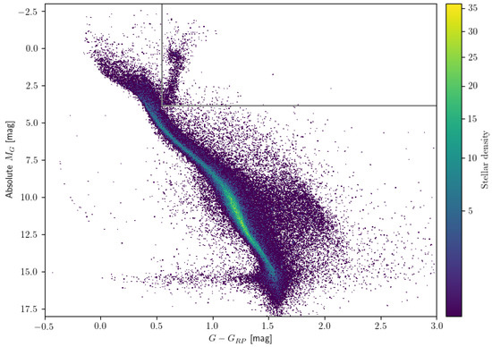
Figure 1.
CAMD for the GCNS (excluded the WD with WDprob > 0.5). The grey lines in the right corner separate the main sequence and the red giants branch.
After these selections, we were left with a final sample of 252,280 stars, of which 130,665 had available radial velocity and magnitudes in Gaia DR3 [10]. In this sample, we converted the equatorial coordinates of proper motions to galactic coordinates and considered the associated uncertainties in positions, parallaxes, and proper motions during the transformation process. Among these 130,665 sources with available proper motions and radial velocity data, we divided the sources into four samples based on their magnitudes as shown in the first column of Table 1.

Table 1.
Measurements of Oort constants in different volumes.
4. Methods
The Oort constants A and B were first defined by [1] under an axisymmetric Milky Way model and later generalized to A, B, C, and K in a non-axisymmetric model by [13]. Ref. [14] made a detailed derivation of the equations. In cylinder coordinates (R, ) with the origin in the galactic center ( increases in the direction of galactic rotation), Oort constants can be expressed as follows:
where and are the mean streaming velocities with respect to R and , respectively. For the local velocity field, Oort constants A and C measure the azimuthal and radial shear, respectively. B and K measure the local vorticity and divergence, respectively.
If the galactic disk is axisymmetric, the Oort constants , and the A and B are:
Thus, measure the local angular velocity
where is the angular velocity of the galactic rotation in the solar vicinity.
In a non-axisymmetric model, the K and C are not zero, and we can get
where is the galactocentric distance of the Sun.
The primary method for determining the Oort constants utilizes their relations to the tangential or radial velocities of local stars. In the solar vicinity, the Oort constantscan be described by the relationship as follows:
where k is the coefficients to convert the proper motion unit from to ; (, ) is the proper motion in galactic coordinates with unit ; d is the solar distance of the star in kpc; the radial velocity is in ; the is the solar velocity in with respect to the LSR. Ref. [14] made a detailed derivation of the relation.
5. Results
To fit the proper motions and radial velocities obtained from GCNS, we utilized a maximum likelihood model. The likelihood function was determined by taking the logarithm and was defined as follows:
where , and are the uncertainties in , and . We considered the velocity dispersion for the distributions in , and , demonstrated by , and , respectively. We assumed a constant velocity dispersion, which did not affect the fitting of the free parameters.
We applied the model to fit proper motions and radial velocities data for each bin and the whole data sample. The final results are presented in Table 1. The uncertainties evaluated by an MCMC method are shown in Figure 2.
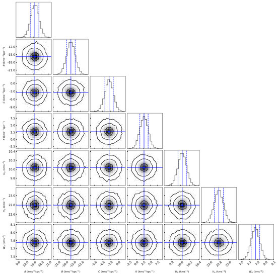
Figure 2.
The MCMC results for (A, B, C, K, , , ) are presented, following the fitting of proper motion data radial velocities for 130,665 stars. The blue lines in each plot represent the mean values adopted for the respective parameters. The top panel in each column displays the probability distribution for each parameter, while the density distribution illustrates the probability density between every pair of parameters. The blue dashed lines displayed in the top panels indicate the ±1 standard deviations.
The best-fitting result determines the Oort constants to be , , and . The parameters (, , ) are calculated as (, , ) . As illustrated in Figure 2, the MCMC results reveal no significant positive or negative correlations among the parameter pairs. Figure 3 displays a comparison between the data and the best-fitting model, indicating a strong alignment between them. The outcomes from various ranges are presented in Table 1. As the range expands, a slight upward trend is observed in the values of A and C, while the changes in B and K remain negligible. The values of (, , ) are entirely independent of , and regardless of how the range of varies, the values of (, , ) consistently remain at (, , ) , which equals the negative mean of all the (U, V, W) of all stars in our sample.
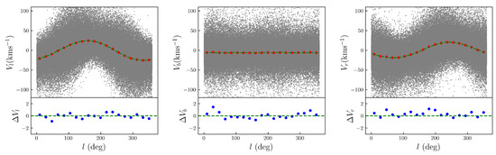
Figure 3.
The panels from left to right display the changes of , , and with respect to the galactic longitude l. The bottom panels demonstrate the residual of the velocity, –. In the top panels, the grey dots represent the velocities obtained from our samples, while the green lines show the results obtained from our best-fitting model and the red dots represent the mean in each galactic longitude bin. In the bottom panels, the blue dots indicate the residual between the data and the model and the green dashed lines illustrate the zero constant velocities.
Table 2 shows the Oort constants results from previous works. The best-fitting value of A aligns with some recent estimates, such as by [14] and by [5]. Nevertheless, this result is slightly smaller than the Gaia DR2 results by [7]. The value of B is , which, in terms of absolute value, is considerably greater than recent research findings by [5,6,7] and marginally less than [14,15]’s earlier figure of . The value of C at , in terms of absolute value, is slightly larger than recent research findings, which indicates the slightly larger radial shear in the immediate vicinity of the Sun (within 100 ). The value of K obtained in our study is positive, whereas other researchers have reported a negative value. This discrepancy may be attributed to the local anomaly or the presence of local velocity streaming, as illustrated in Figure 4. Stellar streams can span vast spatial extents, potentially exceeding 1 [16]. However, the distribution of these streams in space is not uniform, with some areas being densely populated and others sparse. Therefore, when we select a sample in the immediate vicinity of the Sun, we may only be observing a portion of a stellar stream. The velocity distribution of a stellar stream may differ from that of the surrounding stars, which could affect the divergence of the calculated velocity field. If the velocity distribution of a stellar stream deviates from the average velocity distribution of the surrounding stars, it could cause a change in the divergence of the velocity field.
Table 2.
Comparison of Oort constants measurements with previous studies.
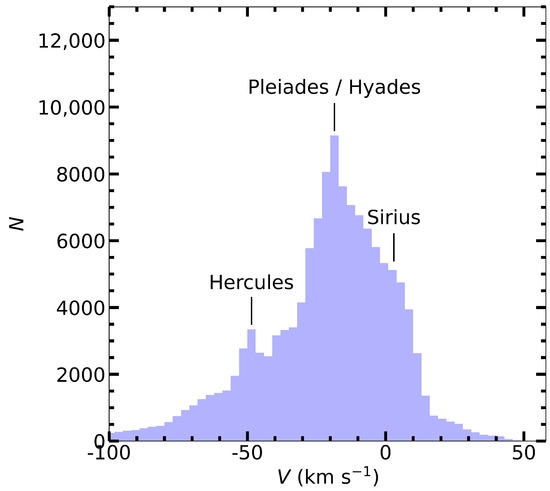
Figure 4.
Distribution of the V velocity components for our sample. Four prominent moving groups are distinctly visible.
The parameters of and represent the peculiar solar motions with respect to the stellar populations. Here, the value at is larger than the majority of recent results shown in Table 3 but smaller than the results of [7,17]. The value of at is in excellent agreement with estimates by [17,18].
Table 3.
Measurements of the solar motion in previous works.
The value does not represent the peculiar solar motion in the V direction, since its determination is more intricate and difficult due to the combination of two factors: solar motion and azimuthal asymmetric drift [26]. The latter represents the average lag concerning the stellar populations. Moreover, as illustrated in Figure 4, the V component of stars is significantly influenced by four well-known moving groups [16] located within close proximity to the Sun (within 100 ), most notably the Pleiades and/or Hyades streams. Owing to the asymmetric drift and the moving groups, the V component displays a subtle asymmetry, with an extended tail toward stars with slower rotation.
The angular velocity , which is consistent with the results obtained with OB stars by [24] but larger than the results found with open clusters by [18]. The , adopting the [27].
6. Discussion and Conclusions
In this study, we have meticulously derived the Oort constants, using a large stellar sample in the solar vicinity from GCNS. This catalog provides a clean sample of stars within 100 of the Sun and is founded on data from the Gaia EDR3. Our sample is substantial, comprising an impressive total of 130,665 stars. We have categorized these sample stars into different magnitude bins for a more granular analysis. Utilizing a maximum likelihood method and a non-axisymmetric model, we computed the Oort constants for each bin. To determine the uncertainties in our calculations, we employed an MCMC method.
The results of our calculations yielded , , and . As for the solar velocity, we determined to be and to be . Furthermore, we computed the angular velocity , which equates to be and the to be . We found that was less than . This indicates that the radial velocity gradient within our star sample is relatively small. This comprehensive analysis of the Oort constants and stellar velocities lays a strong foundation for further studies in the field.
The detection of non-zero values for indicates the presence of a non-axisymmetric distribution within the galactic disk, implying that the distribution of stellar matter is not uniform in all directions. This non-axisymmetry could be the result of various gravitational and dynamic factors, contributing to the complexity of the galactic disk’s structure. Additionally, the computed value of could potentially be influenced by another significant aspect—the existence of the spiral structure in the Milky Way. This structure, a defining characteristic of our galaxy, could contribute to the observed stellar motions and distributions. Significantly, our Sun is located roughly 200 within the ultra-harmonic resonance of this spiral pattern [28]. This location and its dynamical implications are of particular interest. As previously discussed by [29], it is plausible that the gradient in radial velocity, denoted as , could be attributed to the influence of these spiral arms. This effect could cause systematic variations in stellar velocities, an important factor to consider when interpreting our results.
Given these intriguing findings, the relationship between values, the non-axisymmetry of the galactic disk, and the influence of the spiral structure warrants deeper exploration. Further investigations are needed to fully understand these complex dynamics and their implications for our understanding of the Milky Way.
Author Contributions
Conceptualization, Z.Q.; methodology, S.G.; software, S.G.; formal analysis, S.G.; writing—original draft preparation, S.G.; writing—review and editing, Z.Q.; visualization, S.G.; supervision, Z.Q.; funding acquisition, S.G. and Z.Q. All authors have read and agreed to the published version of the manuscript.
Funding
This work is supported by grants from the National Science Foundation of China (NSFC No. 12003025).
Data Availability Statement
This work has made use of data from the European Space Agency (ESA) mission Gaia (https://www.cosmos.esa.int/gaia (accessed on 20 November 2022)). The GCNS catalog can be downloaded from https://cdsarc.cds.unistra.fr/viz-bin/cat/J/A+A/649/A6 (accessed on 20 November 2022).
Acknowledgments
We thank the referee for constructive scientific comments. This work has made use of data from the European Space Agency (ESA) mission Gaia (https://www.cosmos.esa.int/gaia (accessed on 20 November 2022)), processed by the Gaia Data Processing and Analysis Consortium (DPAC, https://www.cosmos.esa.int/web/gaia/dpac/consortium (accessed on 20 November 2022)). Funding for the DPAC has been provided by national institutions, in particular the institutions participating in the Gaia Multilateral Agreement.
Conflicts of Interest
The authors declare no conflict of interest.
References
- Oort, J.H. Dynamics of the galactic system in the vicinity of the Sun. Bull. Astron. Institutes Neth. 1928, 4, 269–284. [Google Scholar]
- Smart, R.L.; Sarro, L.; Rybizki, J.; Reylé, C.; Robin, A.; Hambly, N.; Abbas, U.; Barstow, M.; De Bruijne, J.; Bucciarelli, B.; et al. Gaia Early Data Release 3-The Gaia Catalogue of Nearby Stars. Astron. Astrophys. 2021, 649, A6. [Google Scholar]
- Feast, M.; Whitelock, P. Galactic kinematics of Cepheids from Hipparcos proper motions. Mon. Not. R. Astron. Soc. 1997, 291, 683–693. [Google Scholar] [CrossRef]
- Prusti, T.; De Bruijne, J.; Brown, A.G.; Vallenari, A.; Babusiaux, C.; Bailer-Jones, C.; Bastian, U.; Biermann, M.; Evans, D.W.; Eyer, L.; et al. The gaia mission. Astron. Astrophys. 2016, 595, A1. [Google Scholar]
- Bovy, J. Galactic rotation in Gaia DR1. Mon. Not. R. Astron. Soc. Lett. 2017, 468, L63–L67. [Google Scholar] [CrossRef]
- Li, C.; Zhao, G.; Yang, C. Galactic Rotation and the Oort Constants in the Solar Vicinity. Astrophys. J. 2019, 872, 205. [Google Scholar] [CrossRef]
- Wang, F.; Zhang, H.; Huang, Y.; Chen, B.; Wang, H.; Wang, C. Local stellar kinematics and Oort constants from the LAMOST A-type stars. Mon. Not. R. Astron. Soc. 2021, 504, 199–207. [Google Scholar] [CrossRef]
- Rybizki, J.; Demleitner, M.; Bailer-Jones, C.; Dal Tio, P.; Cantat-Gaudin, T.; Fouesneau, M.; Chen, Y.; Andrae, R.; Girardi, L.; Sharma, S. A Gaia early DR3 mock stellar catalog: Galactic prior and selection function. Publ. Astron. Soc. Pac. 2020, 132, 074501. [Google Scholar] [CrossRef]
- Brown, A.G.; Vallenari, A.; Prusti, T.; De Bruijne, J.; Babusiaux, C.; Biermann, M.; Creevey, O.; Evans, D.; Eyer, L.; Hutton, A.; et al. Gaia early data release 3—Summary of the contents and survey properties. Astron. Astrophys. 2021, 649, A1. [Google Scholar]
- Katz, D.; Sartoretti, P.; Guerrier, A.; Panuzzo, P.; Seabroke, G.; Thévenin, F.; Cropper, M.; Benson, K.; Blomme, R.; Haigron, R.; et al. Gaia Data Release 3 Properties and validation of the radial velocities. arXiv 2022, arXiv:2206.05902. [Google Scholar] [CrossRef]
- Riello, M.; De Angeli, F.; Evans, D.; Montegriffo, P.; Carrasco, J.; Busso, G.; Palaversa, L.; Burgess, P.; Diener, C.; Davidson, M.; et al. Gaia early data release 3—Photometric content and validation. Astron. Astrophys. 2021, 649, A3. [Google Scholar] [CrossRef]
- Lindegren, L.; Klioner, S.; Hernández, J.; Bombrun, A.; Ramos-Lerate, M.; Steidelmüller, H.; Bastian, U.; Biermann, M.; de Torres, A.; Gerlach, E.; et al. Gaia early data release 3—The astrometric solution. Astron. Astrophys. 2021, 649, A2. [Google Scholar] [CrossRef]
- Ogrodnikoh, K. A theory of streaming in the system of B stars. Z. Fur Astrophys. 1932, 4, 190–207. [Google Scholar]
- Olling, R.P.; Dehnen, W. The Oort Constants Measured from Proper Motions. Astrophys. J. 2003, 599, 275–296. [Google Scholar] [CrossRef]
- Comerón, F.; Torra, J.; Gómez, A. On the characteristics and origin of the expansion of the local system of young objects. Astron. Astrophys. 1994, 286, 789–798. [Google Scholar]
- Kushniruk, I.; Schirmer, T.; Bensby, T. Kinematic structures of the solar neighbourhood revealed by Gaia DR1/TGAS and RAVE. Astron. Astrophys. 2017, 608, A73. [Google Scholar] [CrossRef]
- Breddels, M.A.; Smith, M.C.; Helmi, A.; Bienaymé, O.; Binney, J.; Bland-Hawthorn, J.; Boeche, C.; Burnett, B.; Campbell, R.; Freeman, K.C.; et al. Distance determination for RAVE stars using stellar models. Astron. Astrophys. 2010, 511, A90. [Google Scholar] [CrossRef]
- Bobylev, V.; Bajkova, A. Kinematic Properties of Open Star Clusters with Data from the Gaia DR2 Catalogue. Astron. Lett. 2019, 45, 208–216. [Google Scholar] [CrossRef]
- Reid, M.; Menten, K.; Zheng, X.; Brunthaler, A.; Moscadelli, L.; Xu, Y.; Zhang, B.; Sato, M.; Honma, M.; Hirota, T.; et al. Trigonometric parallaxes of massive star-forming regions. VI. Galactic structure, fundamental parameters, and noncircular motions. Astrophys. J. 2009, 700, 137–148. [Google Scholar] [CrossRef]
- Bobylev, V.V.; Bajkova, A.T. Galactic parameters from masers with trigonometric parallaxes. Mon. Not. R. Astron. Soc. 2010, 408, 1788–1795. [Google Scholar] [CrossRef]
- Coşkunoğlu, B.; Ak, S.; Bilir, S.; Karaali, S.; Yaz, E.; Gilmore, G.; Seabroke, G.M.; Bienaymé, O.; Bland-Hawthorn, J.; Campbell, R.; et al. Local stellar kinematics from RAVE data–I. Local standard of rest. Mon. Not. R. Astron. Soc. 2011, 412, 1237–1245. [Google Scholar] [CrossRef]
- Bobylev, V.; Bajkova, A. The local standard of rest from data on young objects with account for the Galactic spiral density wave. Mon. Not. R. Astron. Soc. 2014, 441, 142–149. [Google Scholar] [CrossRef]
- Huang, Y.; Liu, X.W.; Yuan, H.B.; Xiang, M.S.; Huo, Z.Y.; Chen, B.Q.; Zhang, Y.; Hou, Y.H. Determination of the local standard of rest using the LSS-GAC DR1. Mon. Not. R. Astron. Soc. 2015, 449, 162–174. [Google Scholar] [CrossRef]
- Bobylev, V.; Bajkova, A. Kinematics of the galaxy from OB stars with proper motions from the Gaia DR1 catalogue. Astron. Lett. 2017, 43, 159–166. [Google Scholar] [CrossRef]
- Ding, P.J.; Zhu, Z.; Liu, J.C. Local standard of rest based on Gaia DR2 catalog. Res. Astron. Astrophys. 2019, 19, 68. [Google Scholar] [CrossRef]
- Schönrich, R.; Binney, J.; Dehnen, W. Local kinematics and the local standard of rest. Mon. Not. R. Astron. Soc. 2010, 403, 1829–1833. [Google Scholar] [CrossRef]
- Vallée, J.P. Recent advances in the determination of some Galactic constants in the Milky Way. Astrophys. Space Sci. 2017, 362, 79. [Google Scholar] [CrossRef]
- Quillen, A.; Minchev, I. The effect of spiral structure on the stellar velocity distribution in the solar neighborhood. Astron. J. 2005, 130, 576–585. [Google Scholar] [CrossRef]
- Siebert, A.; Famaey, B.; Binney, J.; Burnett, B.; Fauré, C.; Minchev, I.; Williams, M.E.; Bienayme, O.; Bland-Hawthorn, J.; Boeche, C.; et al. The properties of the local spiral arms from RAVE data: Two-dimensional density wave approach. Mon. Not. R. Astron. Soc. 2012, 425, 2335–2342. [Google Scholar] [CrossRef]
Disclaimer/Publisher’s Note: The statements, opinions and data contained in all publications are solely those of the individual author(s) and contributor(s) and not of MDPI and/or the editor(s). MDPI and/or the editor(s) disclaim responsibility for any injury to people or property resulting from any ideas, methods, instructions or products referred to in the content. |
© 2023 by the authors. Licensee MDPI, Basel, Switzerland. This article is an open access article distributed under the terms and conditions of the Creative Commons Attribution (CC BY) license (https://creativecommons.org/licenses/by/4.0/).