Abstract
We consider the central configurations of the -body problem, where N bodies are infinitesimal and the remaining one body is dominant. For regular polygon central configurations, we prove that the masses of all the infinitesimal bodies are equal when N is odd and the masses of the alternate infinitesimal bodies must be equal when N is even. Moreover, in the case of N being even, we present the relationship of the mass parameters between two consecutive infinitesimal bodies.
1. Introduction
The N-body problem is related with the motions of N bodies moving under mutual gravitational attractions and is one of the basic problems in celestial mechanics. Practically, N-body problems can be described by ordinary differential equations [1] as follows:
where is the position of the kth body with mass and is the Newtonian potential function
However, for , this system is very complex and difficult TO SOLVE and there ARE no general solutions; so, people try to search for particular solutions. Central configurations of the N-body problem is one of the most classical topics in celestial mechanics. Central configurations [2] allow us to construct exact solutions for the N-body problem. Collapse orbits and parabolic orbits have relations with the central configurations, and central configurations also have other interesting properties; so, finding central configurations is very important. Central configurations are configurations such that the total Newtonian acceleration of every body is equal to a constant multiplied by the position vector of this body with respect to the center of mass of the configurations.
Definition 1.
A configuration is called a central configuration if q satisfies the following equations:
where ω is some positive constant and assuming the gravitational constant .
is called the configuration space and c is the center of mass, which can be fixed at the origin in the inertial coordinate system.
In this work, we concentrate our interest on the central configurations of the planar restricted -body problem (), where one body is dominant and the other N bodies are infinitesimal, on a plane. Maxwell, J.C. [3] first proposed this problem when he studied Saturn’s rings.
In 1994, Casasayas, J. et al. [4] gave a new derivation of the equations for the central configuration of the body problem. In the case of equal masses, they showed that for a large enough N there exists only one solution. Their lower bound for N improves by several orders of magnitude the one previously found by Hall. In the same year, Moeckel, R. [5] provided a criterion for the linear stability of relative equilibria of the -body problem with N small but not necessarily equal masses. Moreover, he presented several stable periodic orbits of this problem. In 2004, Renner, S. and Sicardy, B. [6] obtained results about the inverse problem—that is, given a configuration, finding the mass parameters and making it a central configuration. They also studied the linear stability and suggested that the presence of co-orbital satellites might explain, at least partly, the confinement of Neptune’s ring arcs. Cors, J. et al. [7] analytically found all the central configurations of the -body problem if the infinitesimal bodies have equal mass when . Numerically, they provided evidence that when the only central configuration is the regular N-gon with the large mass in its barycenter; they also provided evidence of the existence of an axis of symmetry for every central configuration. In 2009, Albouy, A. and Fu, Y. [8] proved that any central configuration of the body problem must be symmetric if the four infinitesimal bodies have equal masses. They also proved rigorously that there are only three such central configurations. In 2011, Corbera, M. et al. [9] considered the -body problem and found two different classes exhibiting symmetric and nonsymmetric configurations. Further, when two infinitesimal masses are equal, they provided evidence that the number of central configurations varies from five to seven. In 2013, Oliveira, A. [10] showed that, for the planar -body problem where the satellites have different infinitesimal masses and two of them are diametrically opposite, the configurations are necessarily symmetric and the other satellites have the same mass. Moreover, he proved that the number of central configurations is, in general, one, two, or three, and in the special case where diametrically opposite satellites have the same mass, they proved that the number of central configurations is one or two and gave the exact value of the ratio of the masses that provides this bifurcation. Xu, X. [11] obtained that there exist at most two kinds of infinitesimal bodies arranged alternately at the vertices of a regular N-gon when N is even, and only one set of identical infinitesimal bodies when N is odd. When and N is even, he found that the regular N-gon relative equilibrium is shown to be linearly stable. When , in 2019, Deng, C. et al. [12] considered symmetric central configurations where the symmetry axis does not contain any infinitesimal mass. Under certain assumptions, they found analytically some central configurations for suitable positive masses and also obtained some numerical results of symmetric central configurations where infinitesimal masses are not necessarily equal. In 2020, Chen, J. and Yang, M. [13] provided criteria for the number of central configurations in the general case, where the masses of the two diametrically opposite satellites are unequal, and drew the bifurcation diagrams. In 2022, Su, X. and Deng, C. [14] studied the relationship between the masses of five infinitesimal bodies and the given symmetric configurations. Under certain assumptions, they found analytically some central configurations for suitable positive masses. Furthermore, they presented some numerical results for configurations and derived the positive masses for these infinitesimal bodies such that these configurations became central configurations.
Next, we will derive the conditional equations for central configuration of the planar -body problem by the method that Moeckel, R. [5] used. Suppose that the dominant body is located at with mass ; the remaining N infinitesimal bodies with positions have masses (), where and is a small parameter that tends to zero. Assume again that the center of mass c is at the origin and is the limiting configuration of the central configuration sequence when tends to zero; then,
so, the limiting position of the dominant body is at the origin when tends to zero.
Notice in Definition 1 that by re-scaling a central configuration we will obtain another one with a different positive constant and there is always a re-scaling factor making . So, the central configuration equations of the -body system become
If , taking the inner product of Equation (1) with gives
Since and , it follows that
so, in all central configurations of this restricted version, the infinitesimal bodies lie on a circle centered at the dominant body, which is at the origin. Let , where is the angle defined by the position of . Taking the inner product of Equation (1) with , dividing by , and taking the limit yields
where is the distance between and .
Take the angles between two consecutive infinitesimal bodies as coordinates, then
In these coordinates, the equations characterizing the central configurations of the restricted -body problem are
where , and .
For the regular polygon central configuration of the restricted body problem (see Figure 1), the angles and Equation (2) become
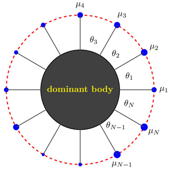
Figure 1.
Configuration of a regular polygon. The blue dots represent the infinitesimal bodies and red dotted line used in the image represents the co-orbital circle.
For the dynamical system (3), we will prove the following:
- (i)
- When N is odd, the mass parameters of all the infinitesimal bodies must be equal, i.e., ;
- (ii)
- When N is even, the mass parameters of the alternate infinitesimal bodies are equal, i.e., and .
This result was obtained by Xu, X. [11] in 2013. He focused his attention on the eigenvalues of the coefficient matrix of system (3); however, the proof is a little obscure and needs calculating software to provide evidence in some places. Here, we will prove the relevant results of eigenvalues in detail by presenting some propositions, corollaries, and lemmas. In addition, we will show in detail how these eigenvalues affect the values of the mass parameters of this system. At the same time, we will give the relationship of the mass parameters between two consecutive infinitesimal bodies when N is even.
2. Propositions and Corollaries
Definition 2.
If an matrix satisfies , and , then A is called a circulant matrix is [15].
According to the definition above, a circulant matrix
Using powers of the fundamental circulant matrix
every circulant matrix A can be represented as
where is the identity matrix.
The characteristic polynomial of the fundamental circulant matrix P is
so, the fundamental circulant matrix P has the eigenvalues
and the corresponding eigenvectors
where is the kth power of the Nth root of unity.
Proposition 1.
The eigenvalues and the corresponding eigenvectors of an circulant matrix are
Proof.
According to the discussion above, the eigenvalues of A can be obtained by the eigenvalues of the fundamental circulant matrix P:
The eigenvectors of A are exactly the same as the eigenvectors of P.
Proposition 2.
The eigenvectors of any circulant matrix form a basis of .
Proposition 3.
The jth power of the Nth root of unity satisfy
This proposition suggests the following formula:
Corollary 1.
.
Proof.
Because , and by Proposition 3, when , the corollary holds. □
Corollary 2.
.
Proof.
The left-hand side equals , by Equation (6), and the two terms of above formula are all zero; thus, the corollary holds. □
3. Preliminary
Define a circulant matrix as follows:
i.e.,
now, Equation (3) is equivalent to
where the mass parameters vector is considered to be unknown.
According to Proposition 1, the eigenvalues of A are
Lemma 1.
(i) When N is even, the eigenvalues of A are
(ii) When N is odd, the eigenvalues of A are
Proof.
Actually, regardless of whether N is even or odd, the eigenvalues of A can be expressed as
where represents the biggest integer that is no greater than the number inside the symbol.
By Lemma 1, it is easy to draw the following corollaries.
Corollary 3.
.
Corollary 4.
.
Proof.
When , by Formula (13),
□
Corollary 5.
When N is even, .
Proof.
By Corollary 4, , which implies . □
Remark 1.
These three corollaries mean that we only need to consider the eigenvalues of A for in the following content, where is the same as above.
Corollary 6.
Proof.
This corollary also suggests that
Because ,
Let
therefore, .
Lemma 2.
For (Roberts, G.E. [16]),
Lemma 3.
(Roberts, G.E. [16]).
4. Theorems and Proofs
According to the discussion in Section 3, we already know that the equations of regular polygon central configuration of the restricted body problem (3) are equivalent to
where A is defined by (8) and is considered to be unknown. In this section, we will study positive real solutions of the linear Equation (18).
Theorem 1.
When N is odd, except ; when N is even, except and .
Proof.
(i) From Corollaries 3 and 5, we already obtain that for every and for even N. Then, by Corollary 4, we just need to study for .
(ii) From the definition of , when , we have that
the first term equals to by Corollary 1 and the second term reduces to
because ; so,
by Lemma 3, , i.e., .
(iii) For ,
by Corollary 2, the first term equals to zero, and by Lemma 2, the second term is greater than zero, which means that , i.e., . Now, the theorem is proven. □
Theorem 2.
Proof.
Because and , it is easy to check that is a solution of (18) for odd N and , is a solution of (18) for even N by direct substitution.
By Theorem 1, when N is odd, except that , which means the rank of A equals to ; so, the general solution of Equation (18) has the form
which is in only if , i.e., .
When N is even, except that and —that is, the rank of A equals to —so, the general solution of Equation (18) has the form
which is in only if and , i.e., and . The proof is completed. □
5. Conclusions
Using the properties of the circulant matrix, we analyzed the eigenvalues of the coefficient matrix of the equations of regular polygon central configuration of the restricted body problem (18) and obtained the positive real solutions of this system. The solutions tell us that for this system, the mass parameters of all the infinitesimal bodies must be equal when N is odd (see Figure 2, all the blue points are equal) and the mass parameters of the alternate infinitesimal bodies are equal when N is even (see Figure 3, alternate blue points need to be equal), these results are a little bit different from the central configuration of regular polygon with a body located at the center for general N-body problems [17]. These results also suggest that geometric symmetry implies physical (mass) symmetry.
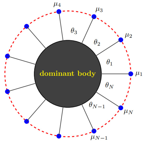
Figure 2.
Central configuration for odd N. The blue dots represent the infinitesimal bodies and red dotted line used in the image represents the co-orbital circle.
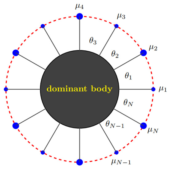
Figure 3.
Central configuration for even N. The blue dots and red dotted line used in the image are as above.
Central configurations of the restricted -body problem are found in several instances in the Solar System. Examples are found in the Saturnian system: one satellite (Helene) librates near the L4 point of Dione; two satellites, Telesto and Calypso, librate near the L4 and L5 of Tethys, respectively; and the co-orbital satellites, Janus and Epimetheus, oscillate in horseshoe orbits around their mutual L3 point. The presence of co-orbital infinitesimal bodies might explain, at least partly, the confinement of Neptune’s ring arcs. However, central configurations of the restricted -body problem do not apply to stellar systems, at least for the entire Solar System. Does it apply to other stellar systems? The answer to this question will be left to future astronomical discoveries.
Author Contributions
Conceptualization, J.C.; formal analysis, J.C. and P.B.; acquisition, J.C., P.B. and M.Y.; methodology, J.C.; project administration, J.C.; software, P.B.; supervision, J.C.; visualization, J.C. and P.B.; writing—original draft, J.C. and M.Y.; writing—review and editing, J.C. and M.Y. All authors have read and agreed to the published version of the manuscript.
Funding
This research was supported by Sichuan Science and Technology Program (grant number 2023NSFSC0079) and the Natural Science Foundation of Southwest University of Science and Technology (grant number 14zx7148).
Data Availability Statement
Data sharing was not applicable to this article as no datasets were generated or analyzed during the current study.
Acknowledgments
The authors sincerely express their gratitude to Shiqing Zhang for his help and guidance.
Conflicts of Interest
The authors declare no conflict of interest.
References
- Saari, D.G. Collisions, Rings and Other Newtonian N-Body Problems; AMS: Providence, RI, USA, 2005; pp. 32–34. [Google Scholar]
- Saari, D.G. On the role and the properties of n body central configurations. Celest. Mech. Dyn. Astron. 1980, 21, 9–20. [Google Scholar] [CrossRef]
- Maxwell, J.C. Stability of the motion of Saturn’s rings. In Maxwell on Saturn’s Rings; Brush, S., Everitt, C.W.F., Garber, E., Eds.; MIT Press: Cambridge, UK, 1983; pp. 1–71. [Google Scholar]
- Casasayas, J.; Llibre, J.; Nunes, A. Central configurations of the planar 1+n body problem. Celest. Mech. Dyn. Astron. 1994, 60, 273–288. [Google Scholar] [CrossRef]
- Moeckel, R. Linear stability of relative equilibria with a dominant mass. J. Dyn. Differ. Equ. 1994, 6, 37–51. [Google Scholar] [CrossRef]
- Renner, S.; Sicardy, B. Stationary configurations for coorbital satellites with small arbitrary masses. Celest. Mech. Dyn. Astron. 2004, 88, 397–414. [Google Scholar] [CrossRef]
- Cors, J.; Llibre, J.; Ollé, M. Central configurations of the planar coorbital satellite problem. Celest. Mech. Dyn. Astron. 2004, 89, 319–342. [Google Scholar] [CrossRef]
- Albouy, A.; Fu, Y. Relative equilibria of four identical satellites. Proc. R. Soc. A 2009, 465, 2633–2645. [Google Scholar] [CrossRef]
- Corbera, M.; Cors, J.; Llibre, J. On the central configurations of the planar 1+3 body problem. Celest. Mech. Dyn. Astron. 2011, 109, 27–43. [Google Scholar] [CrossRef]
- Oliveira, A. Symmetry, bifurcation and stacking of the central configurations of the planar 1+4 body problem. Celest. Mech. Dyn. Astron. 2013, 116, 11–20. [Google Scholar] [CrossRef]
- Xu, X. Linear Stability of the n-gon Relative Equilibria of the 1+n-Body Problem. Qual. Theory Dyn. Syst. 2013, 12, 255–271. [Google Scholar] [CrossRef]
- Deng, C.; Li, F.; Zhang, S. On the symmetric central configurations for the planar 1+4 body problem. Complexity 2019, 2019, 4680716. [Google Scholar] [CrossRef]
- Chen, J.; Yang, M. Central Configurations of the 5-Body Problem with Four Infinitesimal Particles. Few-Body Syst. 2020, 61, 26. [Google Scholar] [CrossRef]
- Su, X.; Deng, C. On the symmetric central configurations for the planar 1+5-body problem with small arbitrary masses. Celest. Mech. Dyn. Astron. 2022, 138, 28. [Google Scholar] [CrossRef]
- Marcus, M.; Minc, H. A Survey of Matrix Theory and Matrix Inequalities; Allyn and Bacon, Inc: Boston, MA, USA, 1964; pp. 1–81. [Google Scholar]
- Roberts, G.E. Linear Stability in the 1+N-Gon Relative Equilibrium. In Hamiltonian Systems and Celestial Mechanics(HAMSYS-98); Delgado, J., Lacomba, E.A., Pérez-Chavela, E., Llibre, J., Eds.; Proceedings of the III International Symposium; World Scientific: Pàtzcuaro, Mexico, 2000; pp. 303–330. [Google Scholar]
- Chen, J.; Luo, J. Solutions of regular polygon with an inner particle for Newtonian N+1-body problem. J. Differ. Equ. 2018, 265, 1248–1258. [Google Scholar] [CrossRef]


Disclaimer/Publisher’s Note: The statements, opinions and data contained in all publications are solely those of the individual author(s) and contributor(s) and not of MDPI and/or the editor(s). MDPI and/or the editor(s) disclaim responsibility for any injury to people or property resulting from any ideas, methods, instructions or products referred to in the content. |
© 2023 by the authors. Licensee MDPI, Basel, Switzerland. This article is an open access article distributed under the terms and conditions of the Creative Commons Attribution (CC BY) license (https://creativecommons.org/licenses/by/4.0/).