Article

Analysis of Pre-Earthquake Ionospheric Anomalies in the Japanese Region Based on DEMETER Satellite Data

1
School of Electronic Information, Wuhan University, Wuhan 430079, China
2
China Research Institute of Radiowave Propagation, Qingdao 266107, China
*
Author to whom correspondence should be addressed.
Universe 2023, 9(5), 229; https://doi.org/10.3390/universe9050229
Submission received: 25 March 2023 / Revised: 7 May 2023 / Accepted: 11 May 2023 / Published: 14 May 2023
(This article belongs to the Section Space Science)

Abstract

:
The electron density (Ne), ion density (Ni), and electron temperature (Te) statistics recorded by the DEMETER satellite payload ISL (Instrument Sonde de Langmuir) were used to study the disturbance characteristics of the ionosphere before solid earthquakes of magnitude 6 or higher in Japan during the summer of 2005 2009 , to provide more information and methods for the coupling mechanism and short-range earthquake prediction. In this paper, the region of ± 10 ° of the epicenter is divided into 1 ° × 1 ° pixels, and the background field of each parameter is constructed using data without earthquakes and relatively calm space weather. We also define a measure of the perturbation intensity of ionospheric parameters relative to the background field during the occurrence of earthquakes. The analysis results of the four Japanese earthquakes from space and time show an excellent synchronization in the time and area of the anomalies in ionospheric parameters of the four cases. All four instances showed Ne abnormalities, and three showed Ni and Te anomalies, in which N e and Ni increased or decreased abnormally, while Te increased abnormally every time, and the anomalies mainly occurred about 9–12 days before the earthquake. This paper eliminates the influence of solar, geomagnetic, and satellite data defects on the experimental results as much as possible in data screening and method selection. The results partially agree with the conclusions reported in the existing literature, and the obtained anomalies are somewhat related to the ionospheric precursors of earthquakes.

1. Introduction

More and more, research results show that the impact of earthquakes on the earth’s environment is not only limited to the Earth’s surface but may also affect the upper atmosphere and ionosphere, causing anomalies in ionospheric electron concentrations and other parameters. With the development of space exploration technology, ionospheric anomalies are receiving more and more attention as a new type of short-range precursor of earthquakes, and there are already articles showing that strong ionospheric disturbances or anomalies occur before strong earthquakes [1,2,3,4].
France launched the DEMETER satellite, the first satellite to provide data for studying ionospheric disturbance information related to earthquakes [5]. Parrot used DEMETER satellite data to repeatedly study the perturbation of electromagnetic waves and ionospheric parameters overhead before the earthquake [6]. Zeng found a sharp change of >20% in Ne and Te near the epicenter 4 and 5 days before the Wenchuan earthquake [7]. Ouyang found that the earthquake causes a synchronous increase in Ne and O+ density [8]. Zhang used DEMETER satellite payload ICE (Instrument Champ Electrique) [9] data to find electrostatic perturbations in the ULF and ELF bands before the earthquake [10]. Yan found that anomalous disturbances of Ne were more easily captured in the seismic region at ± 20 ° equatorial latitude [5]. Yan found that anomalous ionospheric perturbations associated with earthquakes of magnitude greater than 5 were evident at night, and that perturbations in Ni were also observed close to the epicenter after the earthquake [11]. Li mentioned that the sensitivity of Ni to seismic activity tends to be higher than that of Ne [12]. Zheng found that the apparent extent and intensity of ionospheric anomalies increased with increasing magnitude and that post-earthquake ionospheric disturbances were very pronounced [13]. There are many domestic and international studies on the DEMETER satellite, but there are few reports on using it to study pre-earthquake ionospheric anomalies in the Japanese region. Japan is in the earthquake-prone Pacific Rim seismic zone, which is well suited for a statistical study of the changes in ionospheric parameters over earthquakes before multiple strong earthquakes in the same region.
In this paper, the background fields of mean and standard deviation of three ionospheric parameters (Ne, Ni, and Te) were first constructed. Then the ionospheric parameter values of strong earthquakes in Japan from 2005 to 2009 were compared with the background values to obtain the general pattern of ionospheric anomalies in the region before the earthquakes.

2. Data and Shock Example Screening

All publicly available data from the DEMETER satellite can be downloaded from the official website of the French Data Center for Plasma Physics (CDPP: Centre de données de la Physique des Plasmas). This paper uses data from the payload ISL (Instrument Sonde de Langmuir) [14], which contains two types of data, 1143 and 1144, corresponding to plasma parameter data recorded by the satellite in the survey and burst modes, respectively. This paper combines the two data types to form complete orbital data for analyzing ionospheric anomaly information. The screening of ISL payload data is mainly considered from the following two aspects: (1) Since the DEMETER satellite will have missing orbits and data loss in the second half of the service period starting from 2004 and the first half of the retirement period in 2010, and the ionosphere in the mid-latitude area is more sensitive to seasonal changes, this paper mainly uses ionospheric data from the DEMETER satellite ISL payload during the summer period of 2005 2009 (May, June, July, and August) for the study; (2) To avoid the influence of magnetic storms on the experimental results, according to the geomagnetic indices (Dst and Kp), the data under complex space weather with D s t 30   nT and K p 3 are excluded. In addition, since the solar influence on the ionosphere at night is smaller compared to daytime, nighttime data are more suitable for capturing ionospheric anomalies related to earthquakes, and only nighttime data are used in this paper for the study.
According to the earthquake catalog on the official website of the China Earthquake Administration (https://www.cea.gov.cn/cea/index/index.html) (accessed on 24 December 2020), several significant earthquakes occurred in the selected area of Japan during the summer of 2005 2009 , and the earthquake example information is shown in Table 1.

3. Analysis Process

It has been shown that the ionospheric anomalies caused by earthquakes in the gestation process do not necessarily occur over the epicenter but within the gestation zone, and the extent of the gestation zone expands with the increase in magnitude [15,16].
According to the formula for estimating the size of the lithospheric gestation zone proposed by Dobrovolsky [17]:
R = 10 0.43 M
where R is the diameter of the gestation zone in km and M is the earthquake magnitude, the maximum radius of the gestation zone of the earthquake case studied in this paper is about 1377 km (magnitude 7.3). Assuming that the epicenter latitude and longitude are LAT 0 ,   LONG 0 , the size of the study area is selected as LAT 0 ± 10 ° ,   LONG 0 ± 10 ° , and the pixel size is set to 1 ° × 1 ° . Since the ionospheric anomalies are short-lived in time, this paper selects 15 days before the earthquake plus the day of the earthquake as a set of data for studying ionospheric anomalies from the filtered data.
Taking the 6.9 magnitude earthquake (epicenter: 36.7° N, 135.2° E) that occurred in Japan on 16 July 2007, as an example, the parameter Ne is used to illustrate the research method of this paper. First, the statistical background field of the observed parameter Ne is constructed. The study area is 37 °   N ± 10 ° , 135 °   E ± 10 ° and is divided into 400 pixels. The background data are allocated to the corresponding pixels according to the latitude and longitude, and the mean and standard deviation of the data in each pixel are obtained, and 20 × 20 mean matrix β (Figure 1a) and standard deviation matrix σ (Figure 1b) are obtained. Next, the variation field of the observed parameters of the seismic data is constructed. The seismic data are selected from the day of the earthquake and the fifteen days before the earthquake(from 1 July 2007 to 16 July 2007), and only the mean values of the data in each pixel are obtained to obtain a set of 20 × 20 seismic data mean matrices α (Figure 1c). Finally, define the disturbance intensity indicator t.
t = α β σ
The t-value of the data in each pixel is calculated using Equation (2). The calculated results are mapped as color indicators plotted in Figure 1d. In this paper, the process of obtaining t using Equation (2) is referred to as the normalization process of the ionospheric parameter values of the seismic data with respect to the background data. The magnitude of the obtained t-value can measure the intensity of the perturbation of the seismic data to the background field data, and t is a dimensionless indicator. According to the 3σ criterion in statistics, when the magnitude of the parameter t exceeds 3, an ionospheric anomaly is considered to have occurred in the region before the earthquake. The pentagram in Figure 1 indicates the epicenter, and the small black dots in Figure 1c,d show the trajectory of the satellite. The same symbols in the following figures represent the same meaning.

4. Analysis Results and Discussion

4.1. Construction of Background Fields and Seismic-Free Comparison Tests

Background fields were constructed for each of the three ionospheric parameters Ne, Ni, and Te in the ISL load, as shown in Figure 2. It is evident from the mean background fields Figure 2a–c that Te increases with increasing latitude. This pattern of increase with latitude for Ne and Ni is relatively weak, but there is still this regular trend, which is partly consistent with the regularity found by Wang [18] when checking the consistency of ISL ion density data. The overall variation of Ne and Te is smoother compared to Ni, as seen in the standard deviation background fields Figure 2d–f.
To make the anomalous results more objective, the data during the no-earthquake period were divided into 15-day groups and normalized to the background data to obtain the variation of the disturbance intensity index t under the no-earthquake and geomagnetically calm conditions (after data filtering, 15 days of data needs more days to be satisfied, so the time interval in Figure 3 is greater than 15 days). The results of the background data for 2005 are shown in Figure 3. From Figure 3, we can see that the indicator t does not exceed 3 under the no-earthquake condition and the relatively calm space weather condition. A pixel is randomly selected from Figure 3 to plot a time series of three parameters, as shown in Figure 4. As can be seen in Figure 4, the three parameters without a seismic case also have no anomalies over 3 in the time series, and the overall variation of Ne and Ni is relatively consistent. To better understand the correlation degree between the parameters, the background data are assigned to 400 pixels in this paper, and then the correlations between the parameters in each grid are counted and plotted as in Figure 5. The red line in Figure 5 indicates that the Pearson correlation coefficient is 0.7, from which it can be seen that the correlations of Ne and Ni mostly lie on 0.7, showing a strong positive correlation.

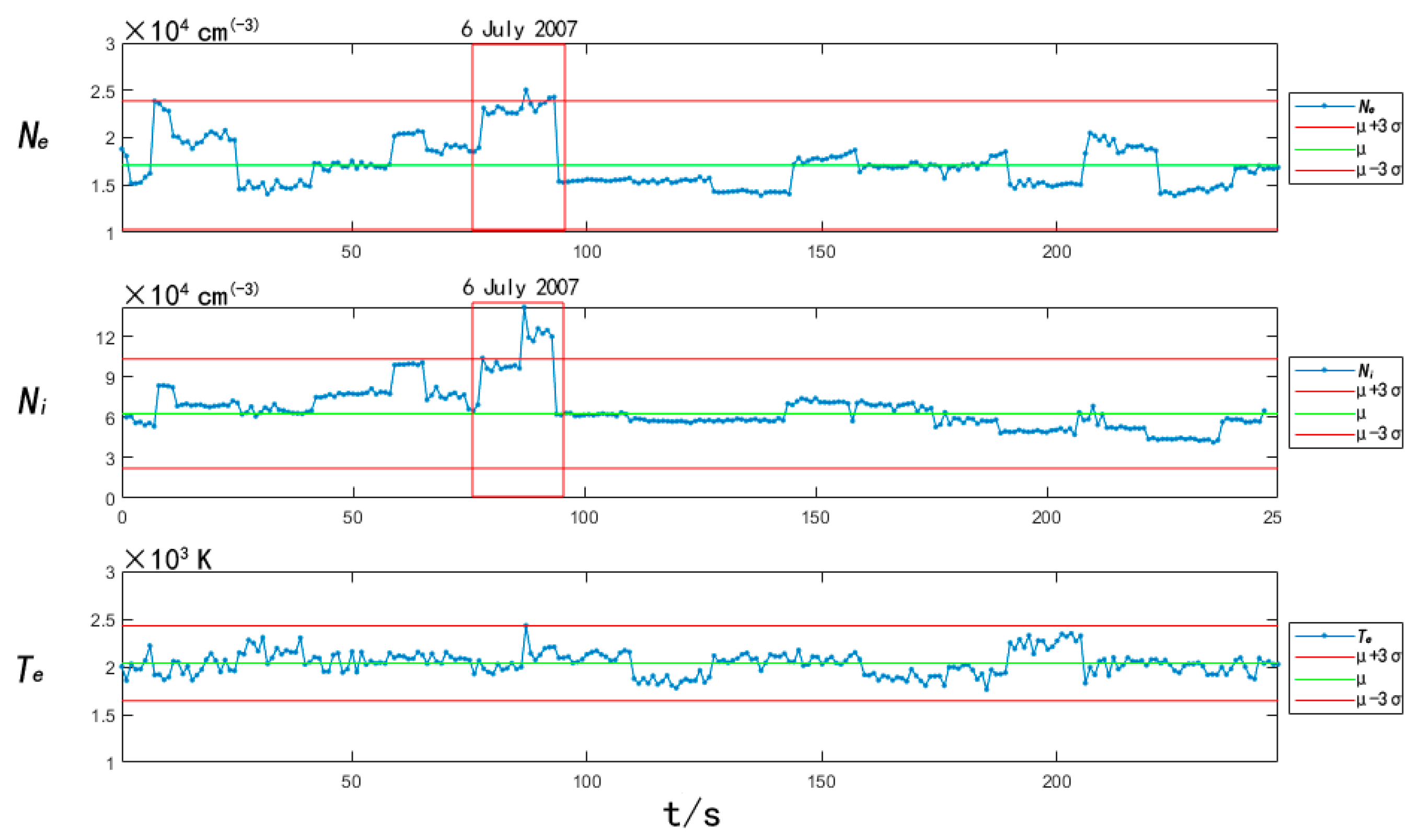
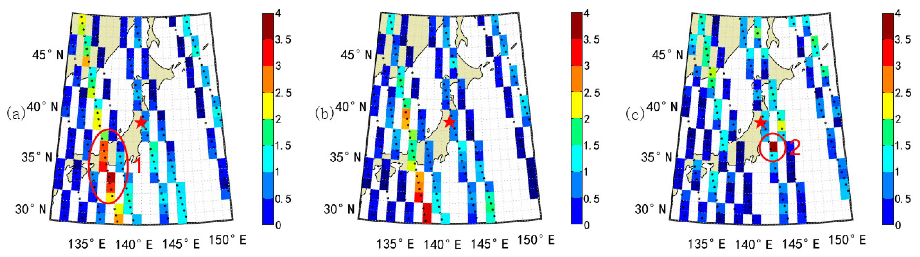
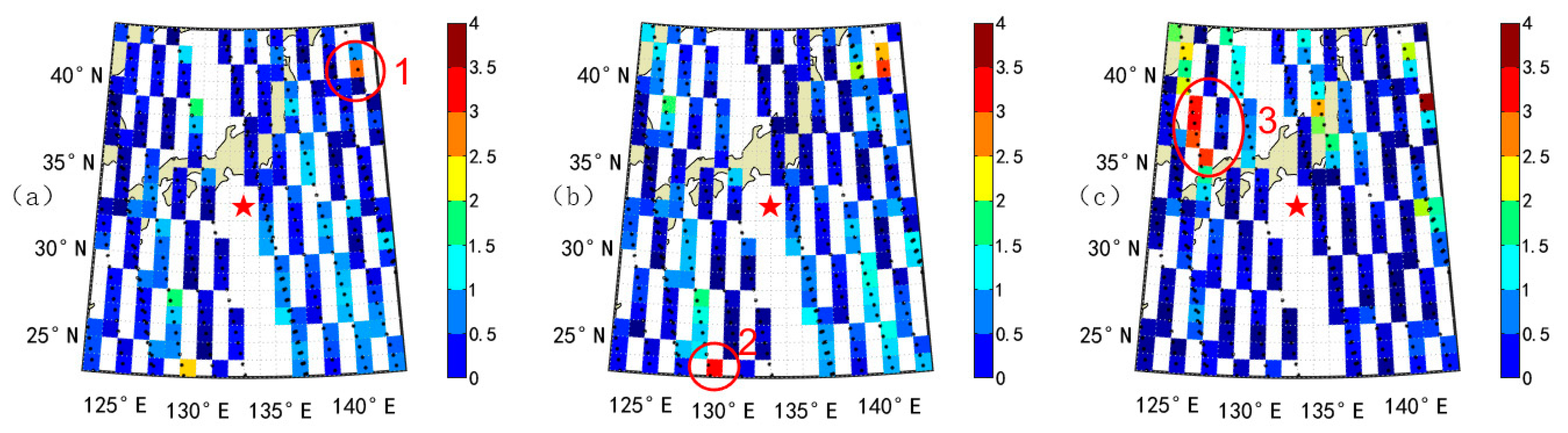
4.2. Earthquake Example 1

The filtered seismic data are normalized to the background field according to Equation (1) for each of the three parameters, and the results are shown in Figure 6. In Figure 6, the pixels with more than 3 anomalies have been circled with red circles and numbered sequentially, and the information of each anomaly region is shown in Table 2. The selected abnormal pixels are marked with red circles and numbers in the subsequent normalized result plots.
Figure 7, Figure 8 and Figure 9 show the curves of the three parameters in the anomalous regions 1, 2, and 3 with time, respectively. From Figure 7, Figure 8 and Figure 9, it can be seen that Ne and Ni showed synchronous anomalous enhancement on the tenth day before the earthquake (6 July 2007); Ni showed anomalous enhancement on the ninth day before the earthquake (7 July 2007), and the magnitude of Ne enhancement was not apparent. Comparing these three time-varying graphs shows that the timing of the anomalies in Ne and Ni is more synchronized. Comparing Figure 3 and Figure 4, it can be concluded that these anomalies may be spatially and temporally related to the current earthquake case. The Te anomaly was not captured in this seismic case study.

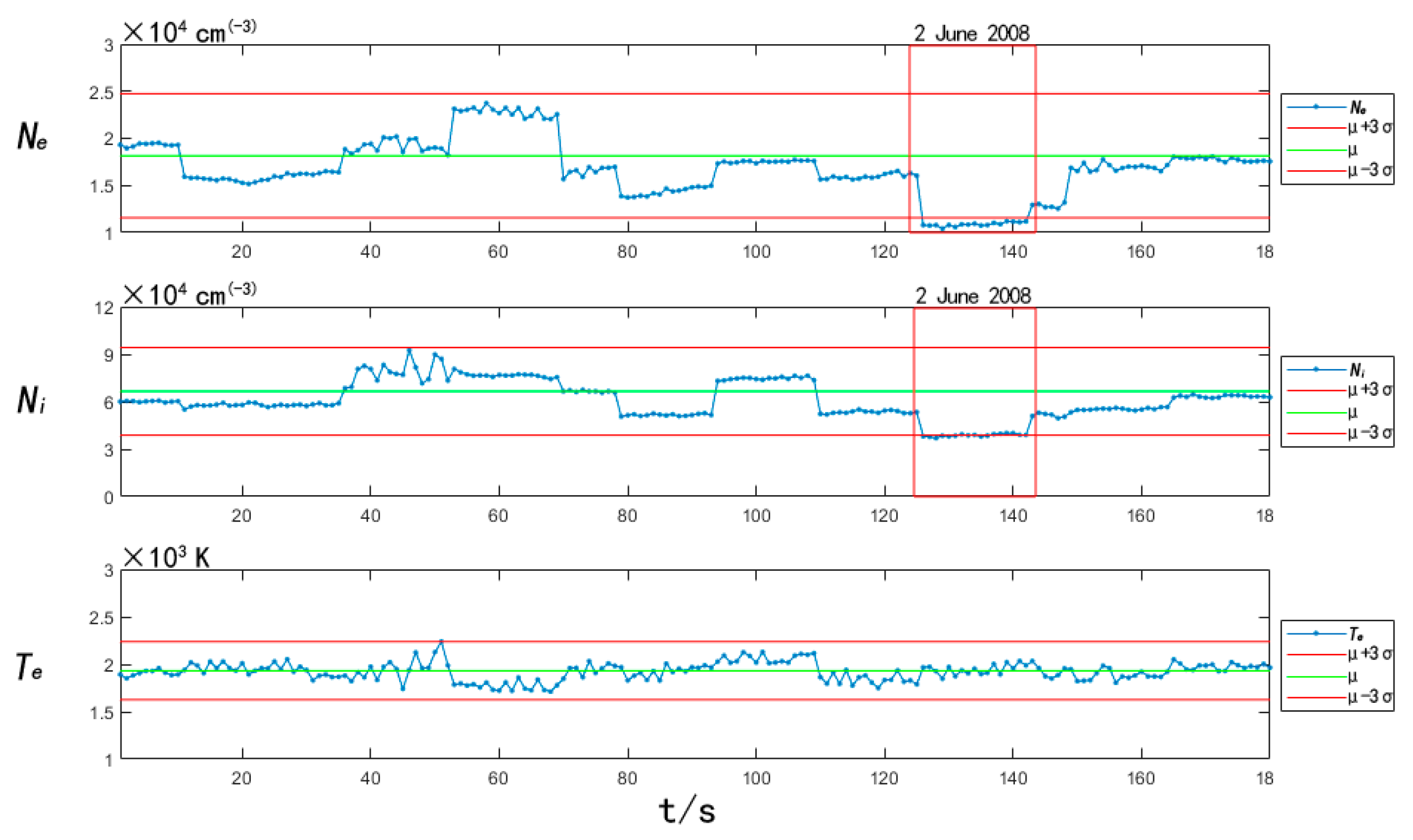
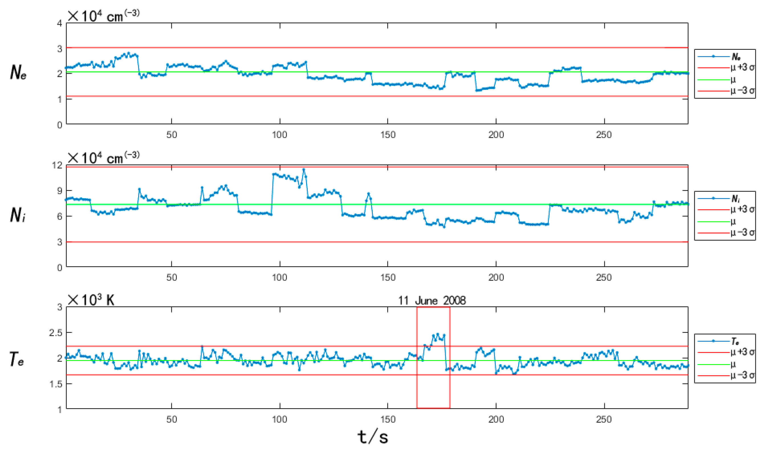
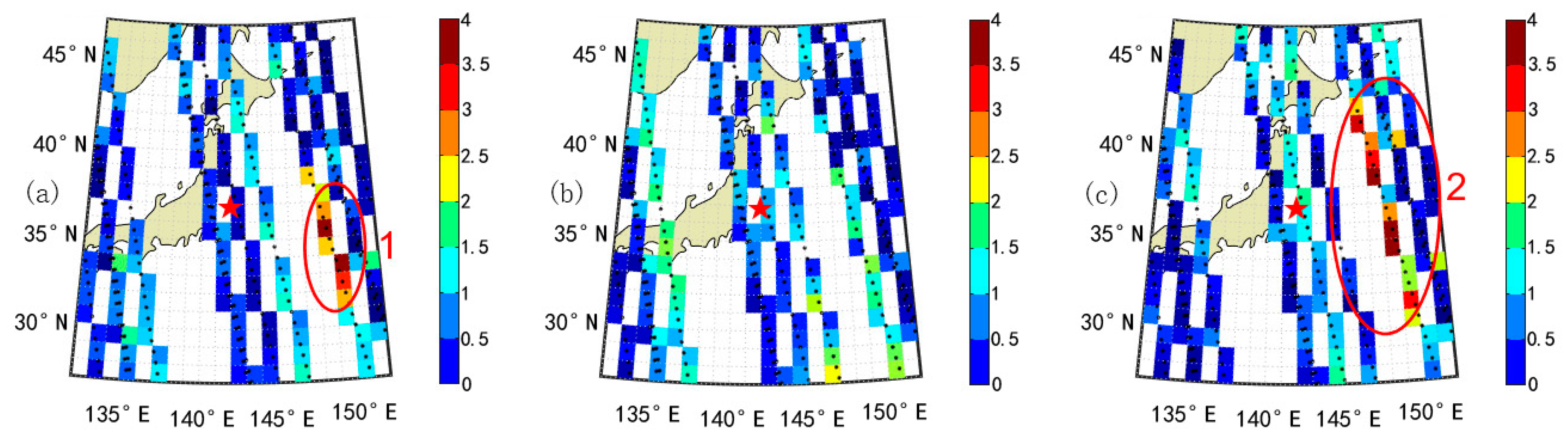
4.3. Earthquake Example 2

The normalized results of the same processing for this earthquake example are shown in Figure 10. Considering that anomalies in the same region of the same track have the same manifestation, for region 1 in Figure 10a, the results of only one pixel are selected to represent the whole region 1. The information on the anomalous regions selected for this earthquake example is shown in Table 3.
Figure 11 and Figure 12 show the curves of the three parameters within the anomalous regions 1 and 2 with time, respectively. By combining Figure 10 and Figure 11, it can be seen that a simultaneous anomalous weakening of Ne and Ni occurred southwest of the epicenter on the twelfth day before the earthquake (2 June 2008). Compared to Figure 3, it can be analyzed that this anomalous weakening phenomenon is closely related to this earthquake example in both time and space dimensions. Combining Figure 10 and Figure 12, it can be seen that on the third day before the earthquake (11 June 2008), Te showed an anomalous strengthening in the southeast direction of the epicenter, while Ne and Ni did not show anomalies at this time.

4.4. Earthquake Example 3

The information on the anomalous region selected for this seismic example is shown in Table 4, and the normalized experimental results are shown in Figure 13.
Combining Figure 13, Figure 14 and Figure 15 shows Ne has an abnormal weakening not only on the third day before the earthquake (16 July 2008) but also on 9 May 2008, and 24 August 2008. Comparing the information of the earthquake cases in Table 1, we can find that the anomalous weakening on 9 May 2008 may be related to the earthquake case on 8 May 2008. Due to the lack of data for the 8 May 2008 example, the case was not studied in depth. We found a strong earthquake with epicenter 41.8 °   N ,   144.0 °   E and magnitude 7.1 occurred in Japan on 11 September 2008. Since this earthquake occurred at a time other than the time interval studied in this paper, this earthquake was not included in the filtered earthquake information. Although the time interval between this phenomenon and the earthquake case is more than 15 days, Ouyang found that the anomaly of Ne reached its maximum 10–20 days before the earthquake [19], so this paper suggests that the anomaly weakened on 24 August 2008, and the earthquake case on 11 September 2008 may be related.
There was no abnormal phenomenon of Ni in this earthquake case, but the synchronous abnormal phenomenon of Ne and Te appeared on the third day before the earthquake (16 July 2008), which was manifested in the abnormal weakening of Ne and the abnormal strengthening of Te.

4.5. Earthquake Example 4

The information on the anomalous region selected for this earthquake example is shown in Table 5, and the normalized experimental results are shown in Figure 16.
Combining Figure 17, Figure 18 and Figure 19, we can see that on the twelfth day before the earthquake (28 July 2009), there was an anomalous enhancement of Te in the northwest region of the epicenter, and Ne and Ni also showed an increase, but the intensity of the increase did not exceed 3. There was an anomalous weakening of Ni in the far southwest region of the epicenter; on the eleventh day before the earthquake (29 July 2009), there was a simultaneous anomalous enhancement of Ne and Ni. The anomalous weakening of Ni on 2 July 2008 was also captured. Since this day was the 18th day after the occurrence of Example 2 and the 17th day before the occurrence of Example 3, whether this anomaly was a post-earthquake effect of Example 2 or a pre-earthquake effect of Example 3 remains to be discussed. These two anomalies may be related to the postseismic effect of this example.

4.6. Anomalies Collation

From Table 6, we can see that the anomalous enhancement of Ne occurs in the north of the epicenter, which is consistent with the conclusion of He [20] that there is an abnormal increase of Ne in the north of the epicenter during the northern hemisphere seismic events, but there is little mention of the anomalous weakening of Ne in the south of the epicenter. Regarding the time of anomalies before the earthquake, some scholars found that the anomalies occurred 1–7 days before the earthquake [21], and some scholars found that the anomalies started 14 days before the earthquake [22]. In contrast, most of the anomalies obtained in this paper occurred about 9–12 days before the earthquake, so conclusions about the time of earthquake precursors need to be studied in many earthquake cases. Combining the results of this paper and the existing research results, it can be seen that some of the parameters appear to be anomalously enhanced and some appear to be anomalously weakened before the earthquake, and the orientation of the region where the anomalies appear is not fixed relative to the epicenter [5,23]. In response to this phenomenon, there is a mechanism of seismic coupling based on the electrostatic field that rocks are constantly subjected to stress during the gestation process of earthquakes, which activates cavity carriers and leads to the accumulation of positive charges on the earth’s surface, thus forming a perturbation electric field E that goes upward from the vertical ground. This perturbation electric field is transmitted to the ionosphere through the atmosphere, and the effect on charged particles in the ionosphere is mainly manifested as a drift phenomenon under the action of E × B . The specific drift direction of charged particles is related to the motion direction of charged particles relative to E × B , which makes the charged particles in the ionosphere anomalously enhanced or anomalously weakened during the earthquake incubation process.

5. Conclusions

In this paper, we construct the background ionospheric field over the Japanese region from which we obtain the background variation pattern of the ionosphere and the variation of the indicator t in the absence of earthquakes. Then we capture and study the anomalous phenomena for each earthquake case from both spatial and temporal latitudes. The conclusions obtained are summarized from the following two aspects:
(1)
Background characteristics
a.
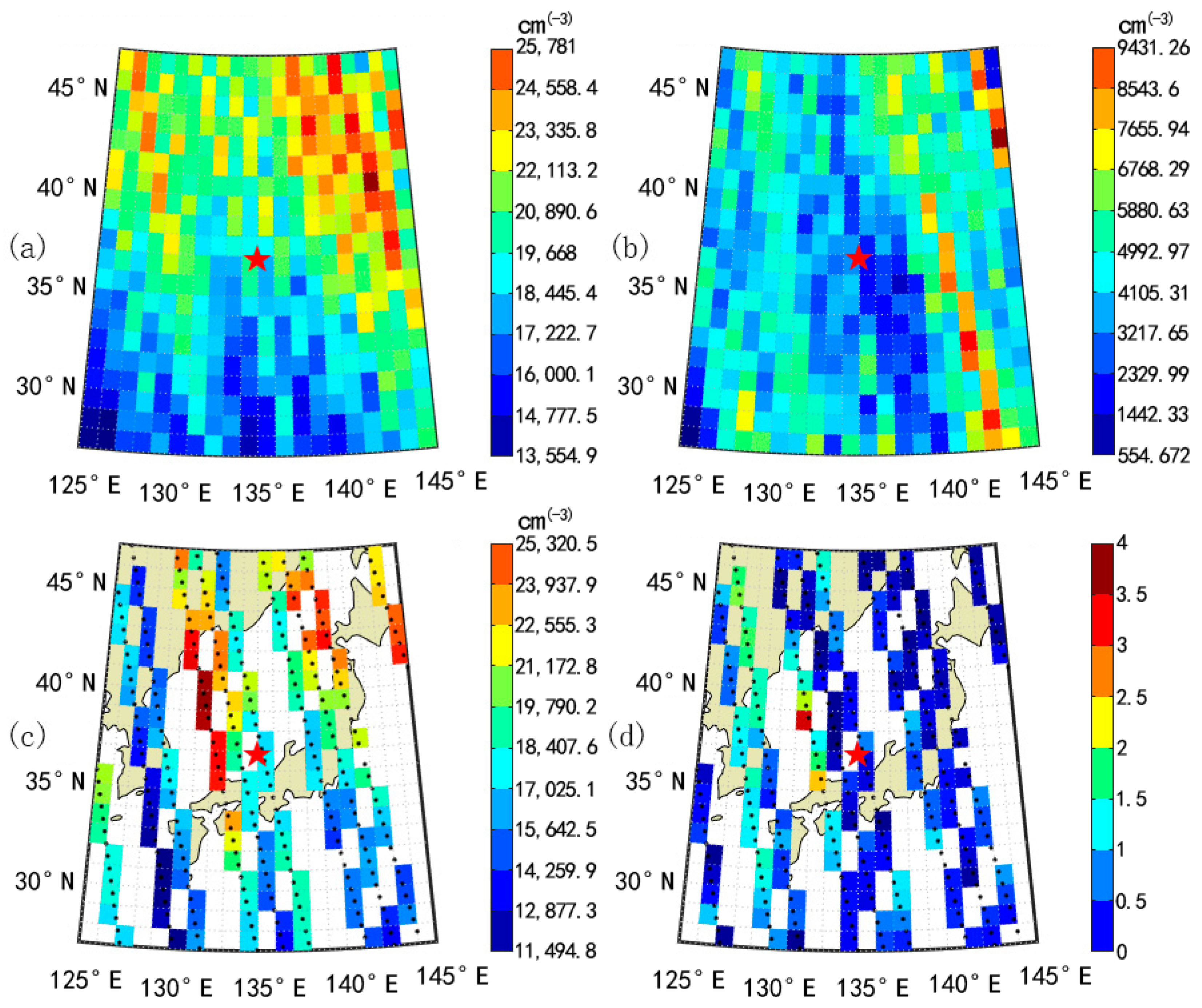
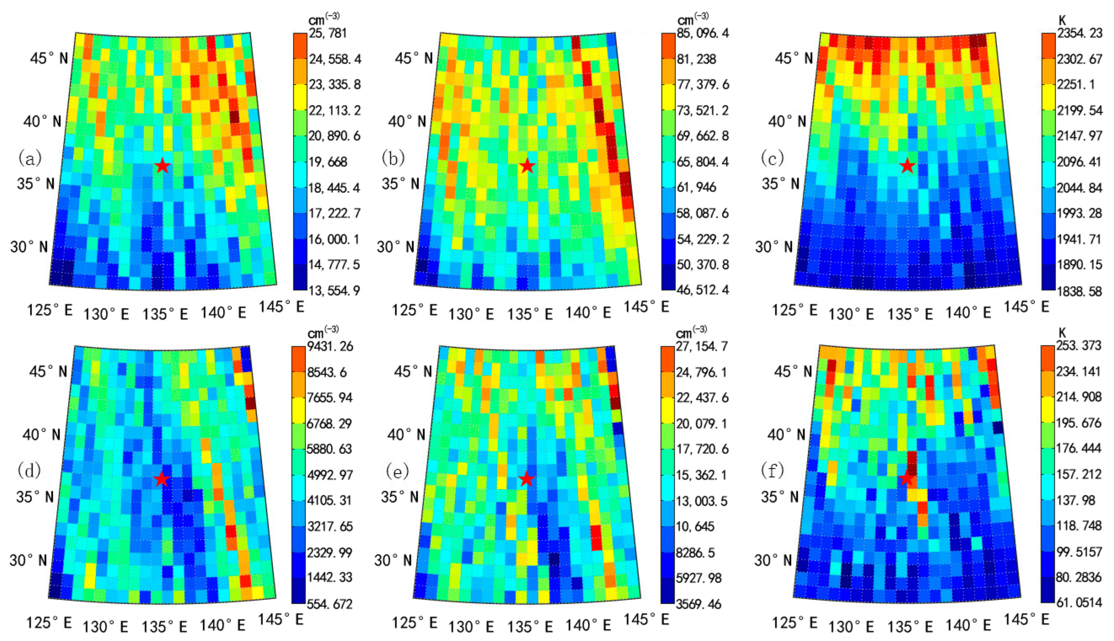
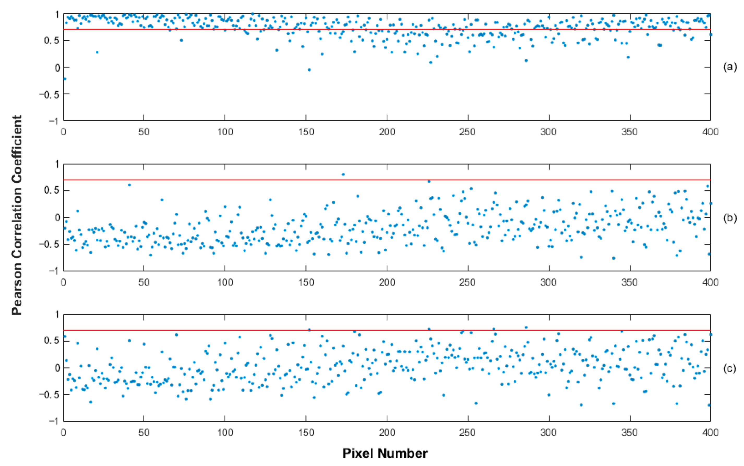
By constructing the background fields of the earthquake cases, it can be seen that Ne, Ni, and Te all have a variation pattern with increasing latitude, and this pattern is more evident for Te and the relatively high correlation between Ne and Ni.
b.
Most of the nocturnal electron concentration values are distributed between 1 ~ 2 × 10 4   cm 3 , most of the ion concentration values are between 4 ~ 8 × 10 4   cm 3 , and most of the electron temperature values are between 1 ~ 2 × 10 3   K .
c.
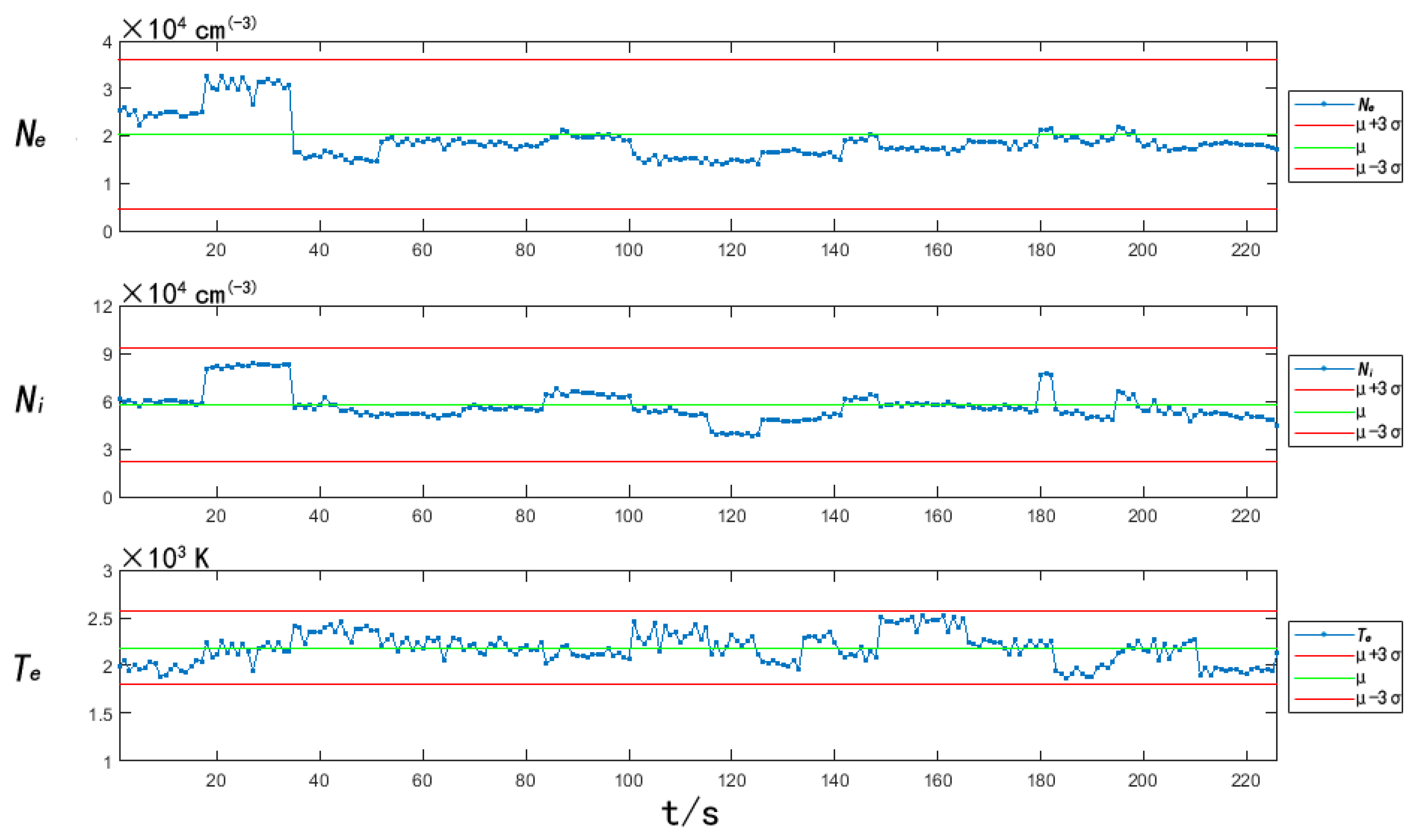
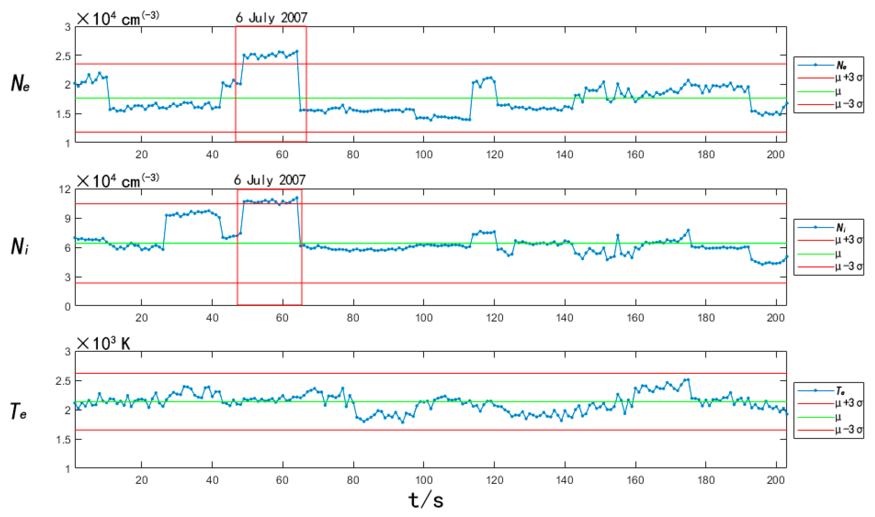
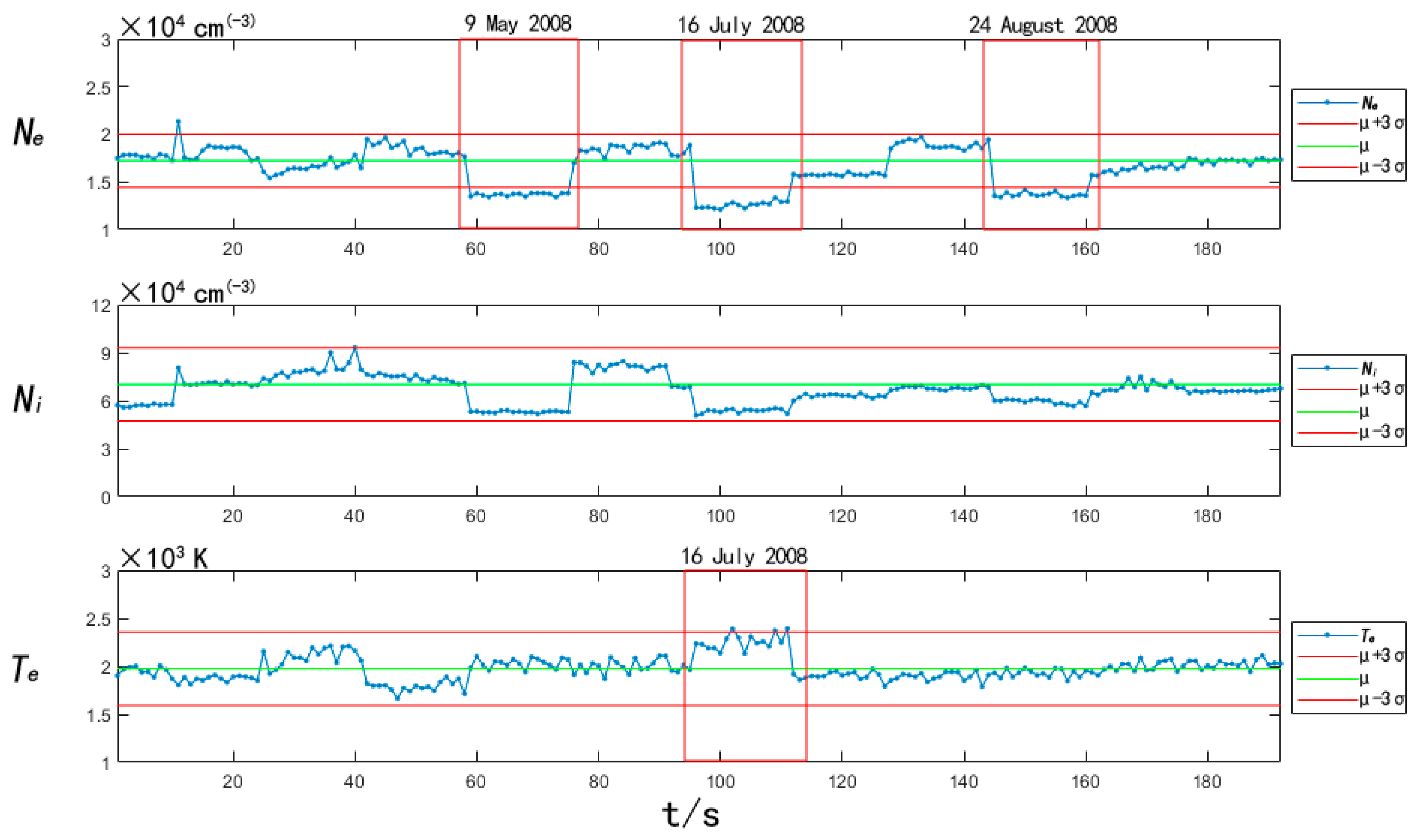
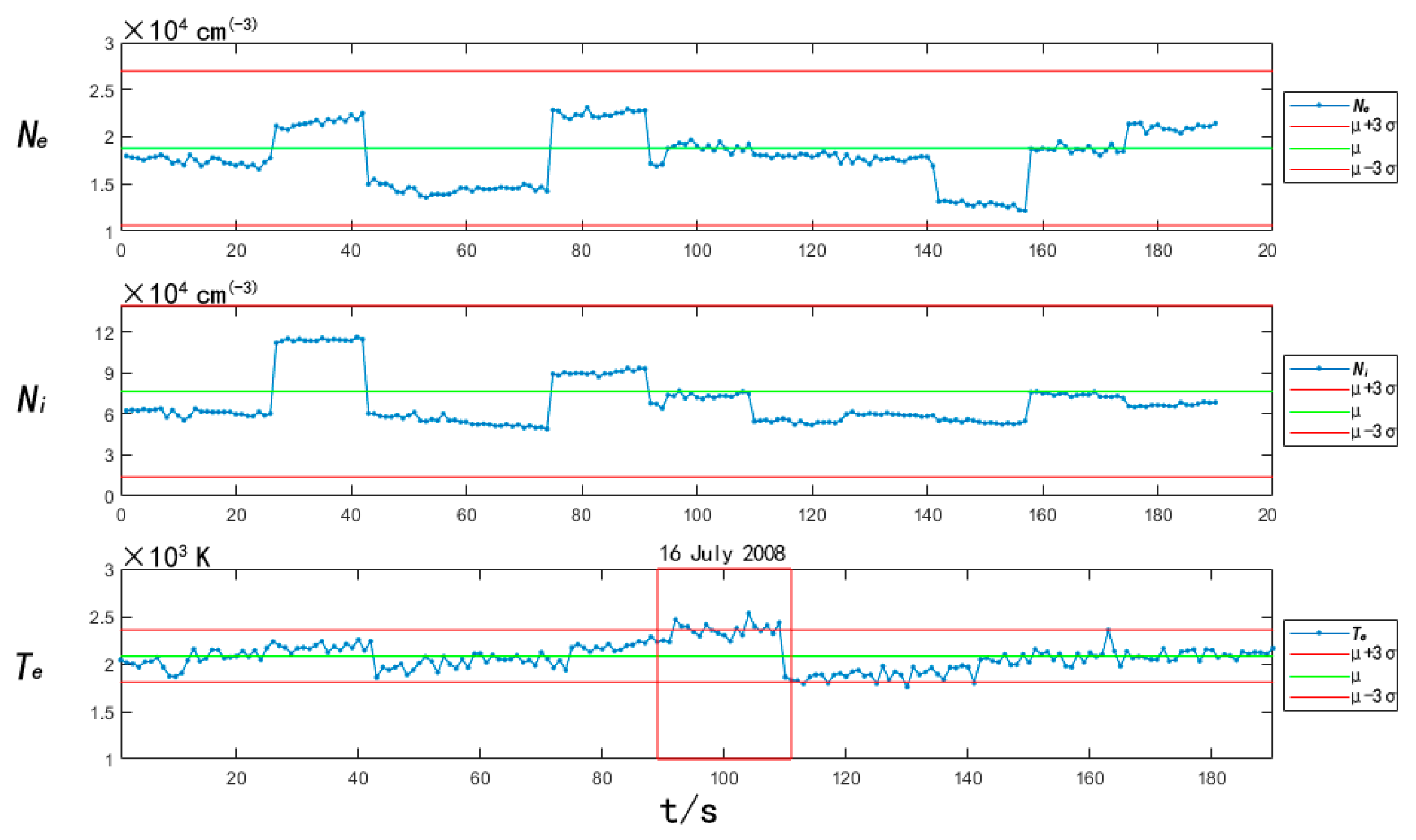
In the case of calm and non-seismic space weather, the perturbation intensity of the three-parameter data relative to the background data is around 1, i.e., no anomalies above 3σ occur in the non-seismic case.
(2)
Anomalies:
a.
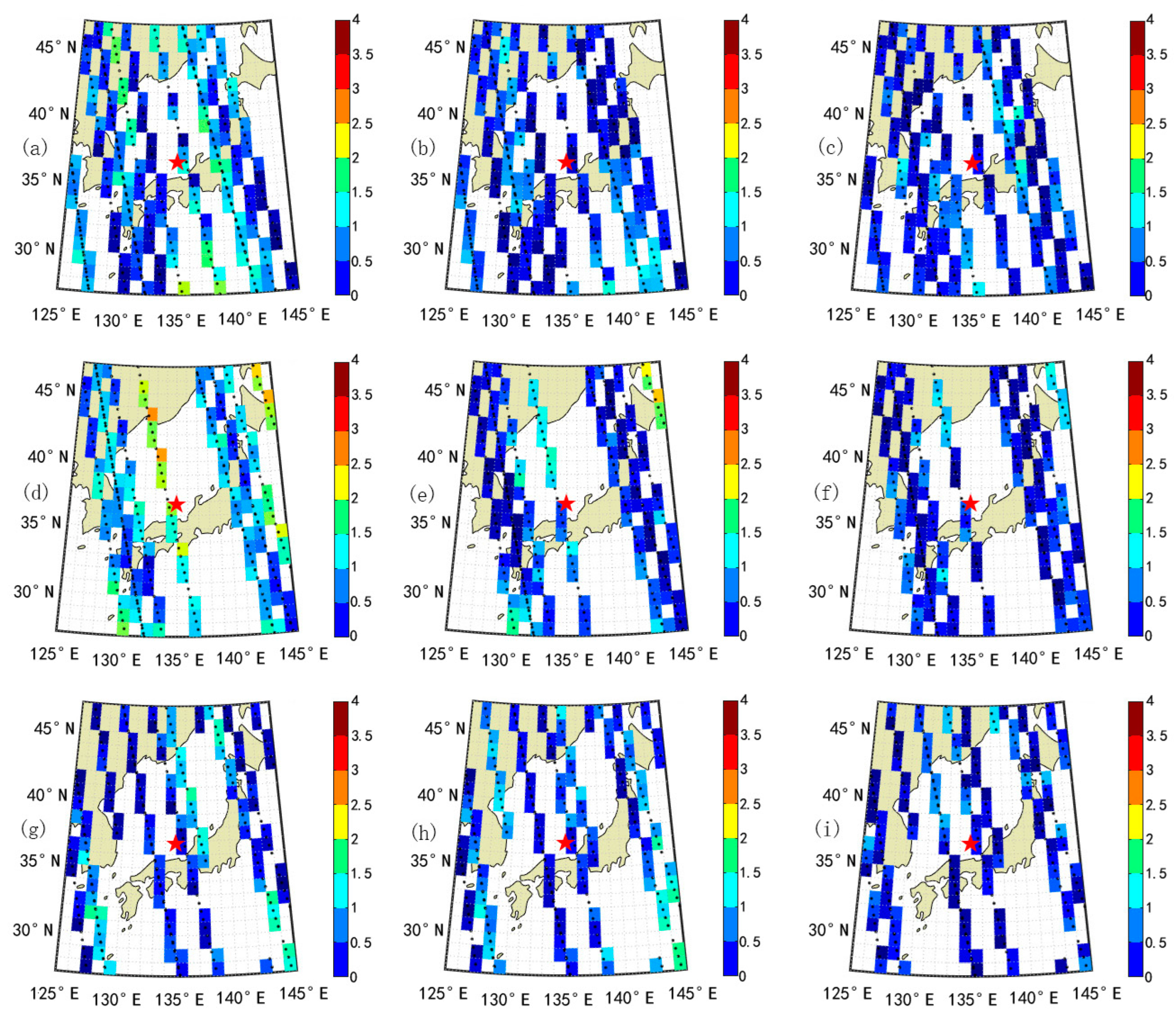
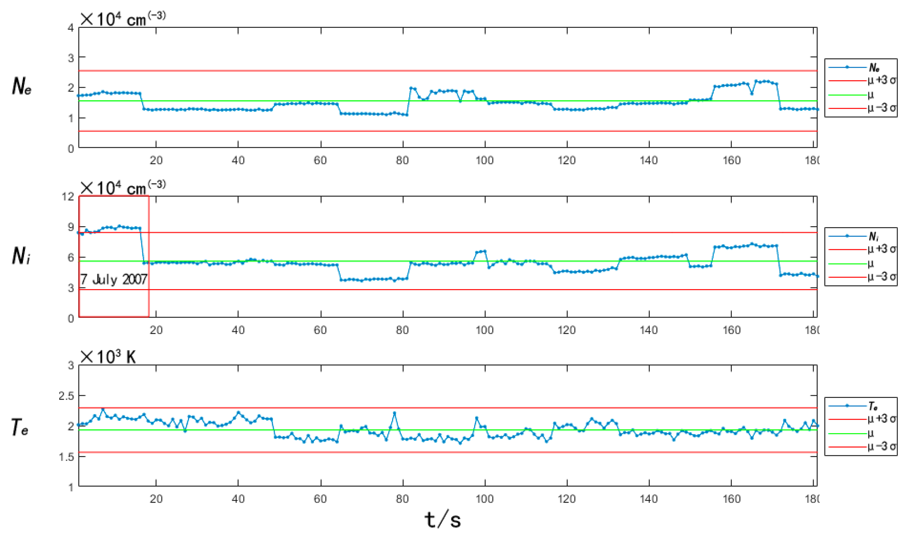
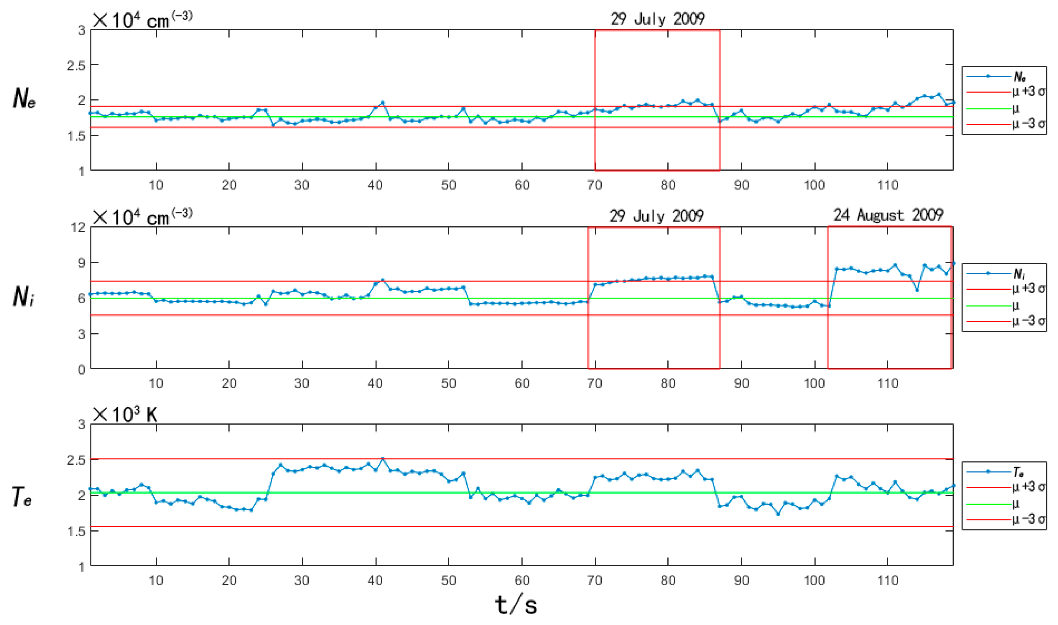
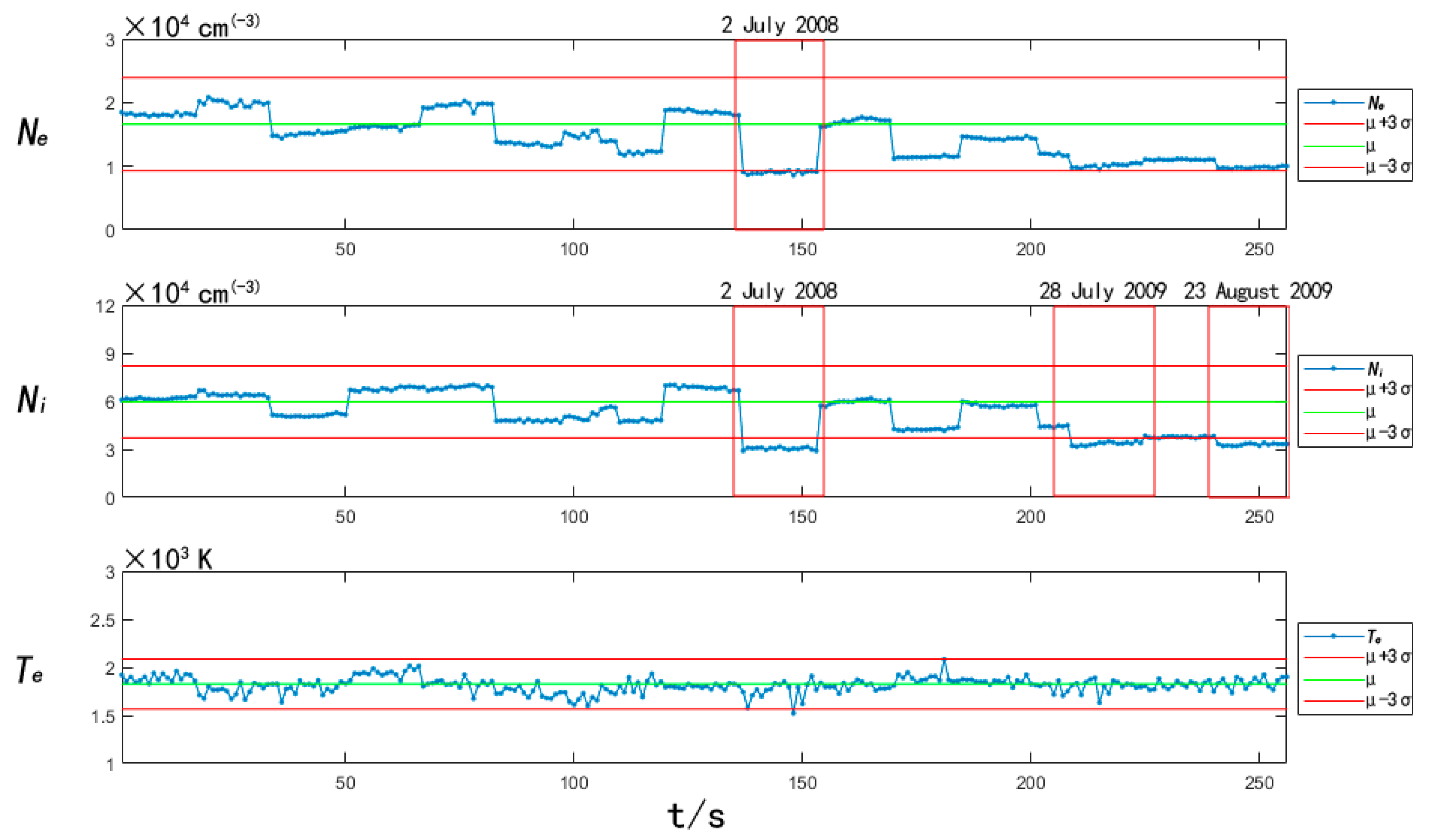
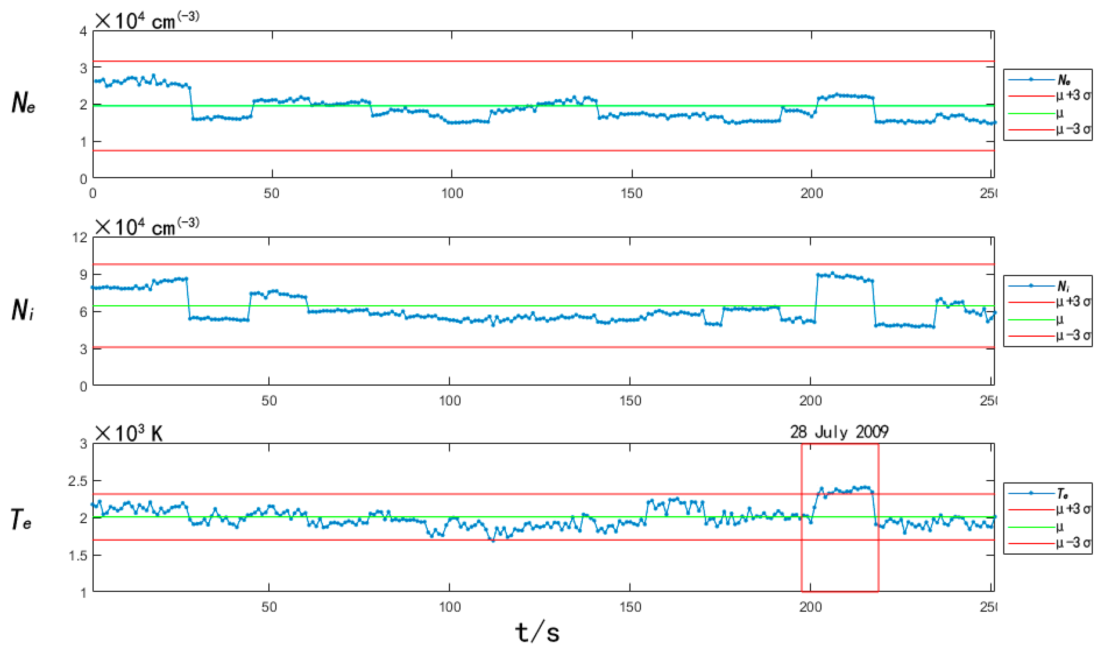
In the four cases studied in this paper, Ne showed anomalies exceeding 3σ, three cases showed Ni and Te anomalies, where Ne and Ni were either anomalously enhanced or weakened before the earthquake, and Te showed anomalous enhancement.
b.
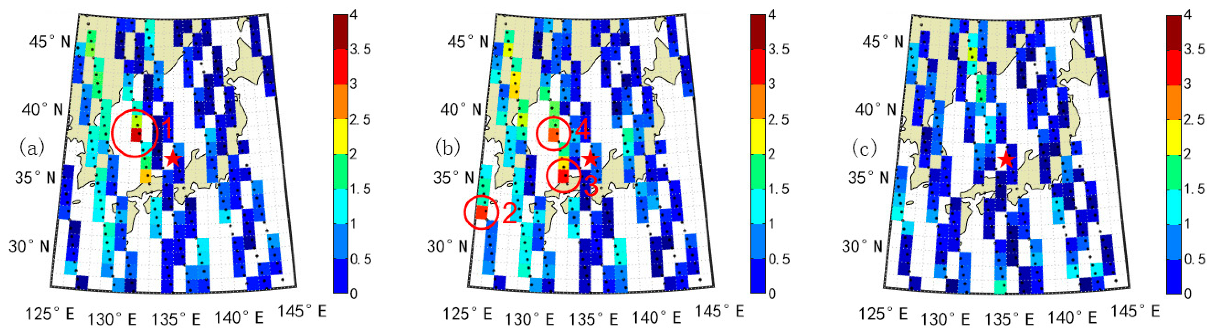
Based on the four earthquake cases, it can be seen that in space, the abnormal enhancement phenomenon of Ne appears in the north of the epicenter, and the abnormal weakening phenomenon appears in the south of the epicenter. The anomalies of Ni and Te are not significantly related to the orientation. In terms of time, the ionospheric anomalies in the three cases appear 9–12 days before the earthquake, and the anomaly in Case 3 appears on the third day before the earthquake. By plotting the variation curves of ionospheric parameters with time, we can obtain that the anomalies can still be captured fifteen days before the earthquake in some cases, which indicates to a certain extent that the earthquake incubation time is more than fifteen days. The spatial orientation and time of the anomalies in the cases studied in this paper show that the earthquake precursors in the same area are also diverse.
c.
For the analysis of the individual earthquake cases, the time and location of the anomalies of the three parameters have a high consistency, especially the anomalous synchronization of Ne and Ni in the same area simultaneously. Combined with the experimental results under no-earthquake conditions, it is reasonable to suggest that there may be a correlation between the occurrence of these anomalies and earthquake incubation.
The diversity and complexity of many conditions, such as geological structure, source mechanism, and ionospheric influences, make earthquake forecasting still a worldwide problem, and we will study more cases in depth in the future to make the results more convincing.

Author Contributions

Conceptualization, Y.H., Z.Z. and Y.Z.; methodology, J.L.; software, J.L.; formal analysis, J.L.; investigation, J.L.; resources, J.L.; data curation, Y.H.; writing—original draft preparation, J.L.; writing—review and editing, C.J. and Z.M. All authors have read and agreed to the published version of the manuscript.

Funding

This work was supported by Stable-Support Scientific Project of China Research Institute of Radiowave Propagation (Grant No. A132001W03).

Data Availability Statement

All the data used in this paper can be viewed and downloaded from the official website of the French Data Center for Plasma Physics (http://demeter.cnrs-orleans.fr/dmt/index.html).

Acknowledgments

Thanks to the DEMETER data center in France for providing the ISL load data for this paper.

Conflicts of Interest

The authors declare no conflict of interest.

References

  1. Chmyrev, V.M.; Isaev, N.V.; Bilichenko, S.V.; Stanev, G. Observation by space-borne detectors of electric fields and hydromagnetic waves in the ionosphere over an earthquake centre. Phys. Earth Planet. Inter. 1989, 57, 110–114. [Google Scholar] [CrossRef]
  2. Molchanov, O.A.; Mazhaeva, O.A.; Golyavin, A.N.; Hayakawa, M. Observation by the Intercosmos-24 satellite of ELF-VLF electromagnetic emissions associated with earthquakes. Ann. Geophys. 1993, 11, 431–440. [Google Scholar]
  3. Pulinets, S.A.; Legen’ka, A.D. Spatial-temporal characteristics of the large scale disturbances of electron concentration observed in the F-region of the ionosphere before strong earthquakes. Cosmic Res. 2003, 41, 221–229. [Google Scholar] [CrossRef]
  4. Parrot, M.; Benoist, D.; Berthelier, J.; Błęcki, J.; Chapuis, Y.; Colin, F.; Elie, F.; Fergeau, P.; Lagoutte, D.; Lefeuvre, F.; et al. The magnetic field experiment IMSC and its data processing onboard DEMETER: Scientific objectives, description and first results. Planet. Space Sci. 2006, 54, 441–455. [Google Scholar] [CrossRef]
  5. Yan, X.X.; Shan, X.J.; Cao, J.B.; Tang, J. Statistical analysis of electron density anomalies before global M7.0 earthquakes (2005–2009) using data of DEMETER satellite. Chin. J. Geophys. 2014, 57, 364–376. (In Chinese) [Google Scholar]
  6. Parrot, M.; Berthelier, J.; Lebreton, J.; Sauvaud, J.; Santolik, O.; Blecki, J. Examples of unusual ionospheric observations made by the DEMETER satellite over seismic regions. Phys. Chem. Earth Parts A/B/C 2006, 31, 486–495. [Google Scholar] [CrossRef]
  7. Zeng, Z.C.; Zhang, B.; Fang, G.Y. The analysis of ionospheric variations before Wenchuan earthquake with DEMETER data. Chin. J. Geophys. 2009, 52, 11–19. (In Chinese) [Google Scholar] [CrossRef]
  8. Xinyan, O.U.; Xuemin, Z.H.; Xuhui, S.H.; Jianping, H.U.; Jing, L.I.; Zhima, Z.E.; Shufan, Z.H. Disturbance of O+ density before major earthquake detected by DEMETER satellite. Chin. J. Space Sci. 2011, 31, 607–617. (In Chinese) [Google Scholar]
  9. Berthelier, J.; Godefroy, M.; Leblanc, F.; Malingre, M.; Menvielle, M.; Lagoutte, D.; Brochot, J.; Colin, F.; Elie, F.; Legendre, C.; et al. ICE, the electric field experiment on DEMETER. Planet. Space Sci. 2006, 54, 456–471. [Google Scholar] [CrossRef]
  10. Zhang, X.; Shen, X.; Parrot, M.; Zeren, Z.; Ouyang, X.; Liu, J.; Qian, J.; Zhao, S.; Miao, Y. Phenomena of electrostatic perturbations before strong earthquakes (2005–2010) observed on DEMETER. Nat. Hazards Earth Syst. Sci. 2012, 12, 75–83. [Google Scholar] [CrossRef]
  11. Yan, R.; Parrot, M.; Pinçon, J.L. Statistical study on variations of the ionospheric ion density observed by DEMETER and related to seismic activities. J. Geophys. Res. Space Phys. 2017, 122, 12421–12429. [Google Scholar] [CrossRef]
  12. Li, M.; Shen, X.; Parrot, M.; Zhang, X.; Zhang, Y.; Yu, C.; Yan, R.; Liu, D.; Lu, H.; Guo, F.; et al. Primary joint statistical seismic influence on ionospheric parameters recorded by the CSES and DEMETER satellites. J. Geophys. Res. Space Phys. 2020, 125, e2020JA028116. [Google Scholar] [CrossRef]
  13. Zheng, L.; Yan, R.; Parrot, M.; Zhu, K.; Zhima, Z.; Liu, D.; Xu, S.; Lv, F.; Shen, X. Statistical Research on Seismo-Ionospheric Ion Density Enhancements Observed via DEMETER. Atmosphere 2022, 13, 1252. [Google Scholar] [CrossRef]
  14. Lebreton, J.P.; Stverak, S.; Travnicek, P.; Maksimovic, M.; Klinge, D.; Merikallio, S.; Lagoutte, D.; Poirier, B.; Blelly, P.L.; Kozacek, Z.M.; et al. The ISL Langmuir probe experiment processing onboard DEMETER: Scientific objectives, description and first results. Planet Space Sci. 2006, 54, 472–486. [Google Scholar] [CrossRef]
  15. Parrot, M.; Mogilevsky, M. VLF emissions associated with earthquakes and observed in the ionosphere and the magnetosphere. Phys. Earth Planet. Inter. 1989, 57, 86–99. [Google Scholar] [CrossRef]
  16. Sharma, D.K.; Rai, J.; Chand, R.; Israil, M. Effect of seismic activities on ion temperature in the F2 region of the ionosphere. Atmosfera 2006, 19, 1–7. [Google Scholar]
  17. Dobrovolsky, I.P.; Zubkov, S.I.; Miachkin, V.I. Estimation of the size of earthquake preparation zones. Pure Appl. Geophys. 1979, 117, 1025–1044. [Google Scholar] [CrossRef]
  18. Wang, X.Y.; Yang, D.H.; Chu, W.; Liu, D.P.; Tan, Q.; Li, W.J.; Shen, X.H. Consistency Validation of the Ion Density Data Obtained by the ISL Payload Onboard DEMETER Satellite. J. Basic Sci. Eng. 2020, 28, 89–102. (In Chinese) [Google Scholar] [CrossRef]
  19. Ouyang, X.Y.; Zhang, X.M.; Shen, X.H. Study on ionospheric Ne disturbances before 2007 Puer, Yunnan of China, earthquake. ActaSeismologica Sin. 2008, 30, 424–436. [Google Scholar]
  20. He, Y.; Yang, D.; Qian, J.; Parrot, M. Response of the ionospheric electron density to different types of seismic events. Nat. Hazards Earth Syst. Sci. 2011, 11, 2173–2180. [Google Scholar] [CrossRef]
  21. Jing, L.; Jianping, H.; Xuemin, Z.; Xuhui, S. Anomaly extraction method study and earthquake case analysis based on in-situ plasma parameters of DEMETER satellite. ActaSeismologica Sin. 2013, 35, 72–83. (In Chinese) [Google Scholar]
  22. Zhang, X.T.; Tursun, N.L.P.; Xia, C.Y. Study on anomaly of ionospheric electron density before the Yushu earthquake using modified pattern informatics method. Recent Dev. World Seismol. 2017, 19–25. (In Chinese) [Google Scholar]
  23. Liu, J.; Wan, W.X.; Huang, J.P.; Zhang, X.M.; Zhao, S.F.; Ouyang, X.Y.; Zeren, Z.M. Electron density perturbation before Chile M8.8 earthquake. Chin. J. Geophys. 2011, 54, 2717–2725. [Google Scholar]
Figure 1. (a) Background mean plot of parameter Ne; (b) Background standard deviation plot of parameter Ne; (c) Mean plot of seismic data of parameter Ne of earthquake case on 16 July 2007; (d) Normalized result plot of parameter Ne of earthquake case on 16 July 2007.
Universe 09 00229 g001
Figure 2. (a) Background mean plot of parameter Ne; (b) Background mean plot of parameter Ni; (c) Background mean plot of parameter Te; (d) Background standard deviation plot of parameter Ne; (e) Background standard deviation plot of parameter Ni; (f) Background standard deviation plot of parameter Te.
Universe 09 00229 g002
Figure 3. (a) Normalized result plot of parameter Ne from 2 May 2005 to 10 June 2005; (b) Normalized result plot of parameter Ni from 2 May 2005 to 10 June 2005; (c) Normalized result plot of parameter Te from 2 May 2005 to 10 June 2005; (d) Normalized result plot of parameter Ne from 11 June 2005 to 19 July 2005; (e) Normalized result plot of parameter Ni from 11 June 2005 to 19 July 2005; (f) Normalized result plot of parameter Te from 11 June 2005 to 19 July 2005; (g) Normalized result plot of parameter Ne from 20 July 2005 to 30 August 2005; (h) Normalized result plot of parameter Ni from 20 July 2005 to 30 August 2005; (i) Normalized result plot of parameter Te from 20 July 2005 to 30 August 2005.
Universe 09 00229 g003
Figure 4. Three-parameter time series without earthquake occurrence.
Universe 09 00229 g004
Figure 5. (a) Statistical plot of correlation coefficients of Ne and Ni; (b) Statistical plot of correlation coefficients of Ne and Te; (c) Statistical plot of correlation coefficients of Ni and Te.
Universe 09 00229 g005
Figure 6. (a) Normalized results plot of parameter Ne of earthquake case on 16 July 2007; (b) Normalized results plot of parameter Ni of earthquake case on 16 July 2007; (c) Normalized results plot of parameter Te of earthquake case on 16 July 2007.
Universe 09 00229 g006
Figure 7. Three-parameter time series plot within anomaly region 1 in seismic example 1.
Universe 09 00229 g007
Figure 8. Three-parameter time series plot within anomaly region 2 in seismic example 1.
Universe 09 00229 g008
Figure 9. Three-parameter time series plot within anomaly region 3 in seismic example 1.
Universe 09 00229 g009
Figure 10. (a) Normalized results plot of parameter Ne of earthquake case on 14 June 2008; (b) Normalized results plot of parameter Ni of earthquake case on 14 June 2008; (c) Normalized results plot of parameter Te of earthquake case on 14 June 2008.
Universe 09 00229 g010
Figure 11. Three-parameter time series plot within anomaly region 1 in seismic example 2.
Universe 09 00229 g011
Figure 12. Three-parameter time series plot within anomaly region 2 in seismic example 2.
Universe 09 00229 g012
Figure 13. (a) Normalized results plot of parameter Ne of earthquake case on 19 July 2008; (b) Normalized results plot of parameter Ni of earthquake case on 19 July 2008; (c) Normalized results plot of parameter Te of earthquake case on 19 July 2008.
Universe 09 00229 g013
Figure 14. Three-parameter time series plot within anomaly region 1 in seismic example 3.
Universe 09 00229 g014
Figure 15. Three-parameter time series plot within anomaly region 2 in seismic example 3.
Universe 09 00229 g015
Figure 16. (a) Normalized results plot of parameter Ne of earthquake case on 9 August 2009; (b) Normalized results plot of parameter Ni of earthquake case on 9 August 2009; (c) Normalized results plot of parameter Te of earthquake case on 9 August 2009.
Universe 09 00229 g016
Figure 17. Three-parameter time series plot within anomaly region 1 in seismic example 4.
Universe 09 00229 g017
Figure 18. Three-parameter time series plot within anomaly region 2 in seismic example 4.
Universe 09 00229 g018
Figure 19. Three-parameter time series plot within anomaly region 3 in seismic example 4.
Universe 09 00229 g019
Table 1. Information on earthquakes.
Earthquake NumberDateEpicenterMagnitudeDepth/kmSpace RangeTime Range
LatitudeLongitudeStart DateEnd Date
116 July 200736.7° N, 135.2° E6.935027–47° N125–145° E1 July 200716 July 2007
8 May 200836.1° N, 141.6° E7.110
214 June 200839.1° N, 140.8° E7.01029–49° N131–151° E30 May 200814 June 2008
319 July 200837.5° N, 142.3° E7.31027–47° N132–152° E4 July 200819 July 2008
49 August 200933.1° N, 138.2° E7.21023–43° N128–148° E25 July 20099 August 2009
13 August 200932.6° N, 140.5° E6.596
Table 2. Earthquake case 16 July 2007 anomalous area information.
Region NumberSpace RangeCorresponding OrbitCorresponding Date
LatitudeLongitude
138–39° N131–132° E16070_16 July 2007
232–33° N125–126° E16085_17 July 2007
335–36° N132–133° E16070_16 July 2007
438–39° N131–132° E16070_16 July 2007
Table 3. Earthquake case 14 June 2008 anomalous area information.
Region NumberSpace RangeCorresponding OrbitCorresponding Date
LatitudeLongitude
132–33° N137–138° E20946_12 June 2008
236–37° N142–143° E21078_111 June 2008
Table 4. Earthquake case 19 July 2008 anomalous area information.
Region NumberSpace RangeCorresponding
Orbit
Corresponding Date
LatitudeLongitude
133–34° N149–150° E21592_116 July 2008
240–41° N147–148° E21592_116 July 2008
Table 5. Earthquake case 9 August 2009 anomalous area information.
Region NumberSpace RangeCorresponding OrbitCorresponding Date
LatitudeLongitude
140–41° N146–147° E27146_129 July 2009
223–24° N134–135° E27132_128 July 2009
338–39° N130–131° E27132_128 July 2009
Table 6. Statistical table of earthquake anomalies.
DateAnomalies
EpicenterNeNiTe
Date and Type of AnomalyAbnormal Area (Relative to the Epicenter)Date and Type of AnomalyAbnormal Area (Relative to the Epicenter)Date and Type of AnomalyAbnormal area (Relative to the Epicenter)
16 July 20076 July 2007 Abnormal enhancementNorthwest6 July 2007 Abnormal enhancement, 7 July 2007 Abnormal enhancementNorthwest and southwest, SouthwestNo abnormalities
36.7° N, 135.2° E
14 June 20082 June 2008 Abnormal weakeningSouthwest2 June 2008 Abnormal weakeningSouthwest11 June 2008 Abnormal enhancementSoutheast
39.1° N, 140.8° E
19 July 200816 July 2008 Abnormal weakeningSoutheastNo abnormalities16 July 2008 Abnormal enhancementSoutheast and southwest
37.5° N,142.3° E
9 August 200929 July 2009 Abnormal enhancementNortheast28 July 2009 Abnormal weakening, 29 July 2009 Abnormal enhancementSouthwest, Northeast28 July 2009 Abnormal enhancement, 29 July 2009 Abnormal enhancementNorthwest, Northeast
33.1° N, 138.2° E
Disclaimer/Publisher’s Note: The statements, opinions and data contained in all publications are solely those of the individual author(s) and contributor(s) and not of MDPI and/or the editor(s). MDPI and/or the editor(s) disclaim responsibility for any injury to people or property resulting from any ideas, methods, instructions or products referred to in the content.

