Article

Approximate Analytical Solutions of the Schrödinger Equation with Hulthén Potential in the Global Monopole Spacetime

by
Saulo S. Alves
1,
Márcio M. Cunha
2,
Hassan Hassanabadi
3,4 and
Edilberto O. Silva
1,*
1
Departamento de Física, Universidade Federal do Maranhão, São Luís 65085-580, MA, Brazil
2
Unidade Educacional de Penedo, Campus Arapiraca, Universidade Federal de Alagoas, Av. Beira Rio, s/n—Centro Histórico, Penedo 57200-000, AL, Brazil
3
Faculty of Physics, Shahrood University of Technology, Shahrood P.O. Box 3619995161-316, Iran
4
Department of Physics, University of Hradec Králové, Rokitanského 62, 500 03 Hradec Králové, Czech Republic
*
Author to whom correspondence should be addressed.
Universe 2023, 9(3), 132; https://doi.org/10.3390/universe9030132
Submission received: 29 October 2022 / Revised: 27 February 2023 / Accepted: 2 March 2023 / Published: 4 March 2023
(This article belongs to the Section Mathematical Physics)

Abstract

:
In this paper, we studied the nonrelativistic quantum mechanics of an electron in a spacetime containing a topological defect. We also considered that the electron is influenced by the Hulthén potential. In particular, we dealt with the Schrödinger equation in the presence of a global monopole. We obtained approximate solutions for the problem, determined the scattering phase shift and the S-matrix, and analyzed bound states.

1. Introduction

The search for exactly solvable models is one of the most relevant tasks in the branch of theoretical physics. However, obtaining exact solutions is not possible in all cases of research interest. In those circumstances, it is necessary to study how to make corrections to these models or even to examine the obtaining of approximate solutions. In the framework of nonrelativistic quantum mechanics, the Schrödinger equation describes precisely the dynamics of a closed quantum system, providing all of the information about the properties of the system [1]. In this context, there are several examples of exactly solvable models, such as the harmonic oscillator [2], the two-body problem with non-central forces [3], the modified ring-shaped oscillator potential [4], and a model involving a class of hyperbolic potential wells [5]. Because of its fundamental feature, it is possible to think about the Schrödinger equation in the most diverse contexts, describing low-dimensional electron gases [6] and problems with anisotropic mass [7], as well as the presence of curvature and torsion in the spacetime [8]. Concerning the Schrödinger equation in a curved space, a relevant type of problem consists of studying the presence of topological defects [9]. Topological defects can arise in the contexts of gravitation and condensed matter physics. In the first one, topological defects are associated with the process of evolution in the early universe, in which symmetry-breaking phase transitions took place [10]. In condensed matter physics, these defects might appear during material synthesis, being inevitable in the process [11]. The study of the physical implications of these defects on the physical properties of a system has been an active research line in the last few decades.
In gravitation, we can cite topological defects such as cosmic strings, domain walls, and global monopoles [9,12,13]. As pointed out in [14], cosmic strings and global monopoles are exotic topological defects. Around a cosmic string, spacetime is not globally flat but locally flat. Another remarkable feature about cosmic strings refers to the fact that we can associate a conical geometry to this type of defect. Because of this, there is a counterpart for cosmic strings in condensed matter physics, which is named disclinations [15,16]. A disclination also presents a conical geometry that manifests in solids and liquid crystals. The spacetime of cosmic string exerts an impressive influence on the behavior of a physical system, in which effects such as gravitational leasing, self-force, and the gravitational Aharonov–Bohm effect take place. In the literature, different models have been solved in the cosmic string spacetime [17,18,19,20,21,22,23,24,25,26,27,28,29,30,31,32,33] and disclinations [34,35,36,37,38,39,40,41], demonstrating the wide range of possibilities of investigation involving these issues.
A global monopole also presents significant features, such as the topological scattering of test particles. For this defect, one can say that its influence manifests because of a solid deficit angle that dictates the corresponding spacetime’s topological behavior and curvature. In condensed matter physics, topological defects might appear in various scenarios; for instance, as domain walls in magnetic materials, vortices in superconductors [42], and solitons in polyacetylene [43]. In addition, there are defects known as dislocations that occur in disordered solids [12,44]. In the present manuscript, we are interested in studying the influence of a spacetime produced by a global monopole on the quantum mechanics of a nonrelativistic particle. For a global monopole, the scalar matter field plays the role of an order parameter where, outside the monopole, the core acquires a non-vanishing value. In this context, Barriola and Vilenkin [45] presented an approximate solution of the Einstein equations [46,47,48] for the metric outside a monopole resulting from the global  O ( 3 ) symmetry breaking. They showed that the monopole exerts practically no gravitational force on the nonrelativistic matter. In addition, the space around it has a solid angle deficit, and the same angle, independent of the impact parameter, deflects all light rays. After this study, several works were developed in this direction, including the study of the polarization and vacuum fluctuations [49,50,51], relativistic motion of quantum oscillator [52,53,54], radiation, absorption and scattering of black holes [55,56,57], etc.
As we have mentioned, the study of quantum mechanics problems in which the Schrödinger equation has no exact solutions is a question of interest due to its foundational character. To deal with these problems, it is often necessary to implement approximation techniques. As examples of investigations in this context, we can cite solutions of the Schrödinger equation with Eckart plus inversely quadratic Yukawa potentials [58], Hua plus modified Eckart potential with the centrifugal term [59], Manning–Rosen plus Hellmann potential and its thermodynamic properties [60], and the shifted Deng–Fan potential model [61]. Then, studying the nonrelativistic quantum motion of a particle in the presence of both the Hulthén potential and the global monopole is a pertinent issue.
With all of this in mind, in this manuscript, our goal consisted of obtaining approximate solutions for the Schrodinger equation in the spacetime of a global monopole in the presence of the Hulthén potential. That potential class presents an extensive scope of applications, such as nuclear physics, chemical physics, and condensed matter systems [62]. Regarding the study of approximate solutions when the Hulthén potential is present, we can cite examples of works in the literature dealing with this topic in the framework of the Schrödinger equation [63], Klein–Gordon equation [64], and Dirac equation [65,66].
The organization of the paper is as follows. In Section 2, we write the Schrödinger equation for a charged particle in the global monopole spacetime, including the Hulthén potential. Before solving the radial equation, we study the effective potential to which the particle is subjected. We show that bound states are allowed for  α < 1 and  α > 1 , and the other parameters are fixed. To solve the radial equation of motion for arbitrary states, we used standard approximations to the Hulthén potential. We show that the radial differential equation is of the hypergeometric type, and its solution is given in terms of the hypergeometric function  2 F 1 a , b ; c ; z . In Section 3, we solve the radial equation for scattering states and find the phase shift of the wave function. Section 4 is dedicated to examining bound states solutions. To achieve this, we first determined the S-matrix and then analyzed its poles, from which, an expression for the energy of bound states could be obtained. We end this section by presenting some sketches for the energy levels and comparisons with other results in the literature. Finally, we make our concluding remarks in Section 5.

2. Nonrelativistic Quantum Mechanics in the Global Monopole Spacetime

In this section, we write the Schrödinger equation with vector coupling to describe the motion of an electron interacting with the Hulthén potential in the global monopole spacetime. The metric of this manifold is expressed by the line element [45]
d s 2 = d t 2 + α 2 d r 2 + r 2 d θ 2 + sin 2 θ d φ 2 ,
where  α 2 = 1 8 π G η 2 is smaller than 1 and represents the deficit solid of this manifold. The parameter  η corresponds to the scale of gauge-symmetry breaking [67]. For this spacetime, it is known that the area of a sphere of unit radius is not  4 π r 2 but  4 π α 2 r 2 . Furthermore, the surface with  θ = π / 2 presents the geometry of a cone (gauge cosmic string) with a deficit angle  Δ ˜ = 8 π 2 η 2 . It is known that the motion of massive or charged particles in the spacetime (1) involves the effect of the self-interaction potential in the model description. In this case, the relevant equation is the Schrödinger equation in spherical polar coordinates with vector coupling. The Schrödinger equation has the form
H ψ = E ψ ,
where H is the corresponding Hamiltonian operator, given by
H = 1 2 M p 2 + V e f f r .
Here, p denotes the momentum operator, M is the mass of the particle, and
V e f f r = V H r + V S I r
is the effective potential, which contains the Hulthén potential  V H r and the electrostatic self-interaction potential  V S I r . The self-interaction potential  V S I r is of the Coulomb-type, given by [68]
V S I ( r ) = K α r ,
where r is the distance from the electron to the monopole and  K ( α ) is the constant of coupling. In a general analysis, depending on the sign of  K ( α ) , the potential  V S I ( r ) can be either attractive or repulsive. For the electrostatic case,  K ( α ) is known to be [68]
K α = e 2 S ( α ) 2 > 0 ,
where e is the electron charge. The function  S ( α ) is given by
S ( α ) = l = 0 2 l + 1 4 l l + 1 + α 2 1 ,
where l denotes the angular-momentum quantum number. Note that  S ( α ) is a finite positive number for  α < 1 and negative for  α > 1 . In our approach, we consider these two possibilities for  α and discuss the physical implications when  V S I ( r ) is added to the Hulthén potential in its approximate form, which we present later. Although the case with  α > 1 is nonphysical, we consider it important because it makes our study more complete from a mathematical physics point of view. The Hulthén potential is given by [69,70]
V H r = Z e 2 ξ e ξ r 1 e ξ r ,
where Z is a positive constant and  ξ is the screening parameter that determines the Hulthén potential range. When the potential  V H ( r ) is used for atoms phenomena, the constant Z is identified with the atomic number. Some authors have opted to define a new parameter, namely  V 0 = Z e 2 ξ , and state that  V 0 is related to the atomic number Z and the screening parameter  ξ [71]. Here, we prefer to conduct these parameters explicitly in our calculations as in Reference [72]. With the inclusion of the effective potential (4), Equation (2) can be written explicitly as
2 2 M α 2 r 2 r r 2 r L 2 r 2 ψ r + K α r ψ r Z e 2 ξ e ξ r 1 e ξ r ψ = E ψ r ,
where  L is the usual orbital angular momentum operator in spherical polar coordinates. At this point, it is useful to notice that  H , L = H , L 2 = 0 . From these commutation relations, together with Equation (2), we can write the following equations [73] involving the angular momentum operator and its corresponding quantum numbers:
L 2 ψ r = l l + 1 2 ψ r ,
L z ψ r = m ψ r .
In this way, we shall search for energy eigenstates of the form
ψ r = R n r Y l m θ , φ ,
in which  Y l m θ , φ represents the spherical harmonics functions. Substituting this solution into Equation (9) together with the standard change in variables  R r = r 1 u ( r ) , we obtain the radial equation
2 α 2 2 M d 2 u ( r ) d r 2 + V e f f u ( r ) = E u ( r ) .
where
V e f f ( r ) = 2 2 M l l + 1 r 2 + K α r Z e 2 ξ e ξ r 1 e ξ r .
and  K α is given in Equation (6). Equation (13) is the Schrödinger equation in the spacetime of a global monopole in the presence of the Hulthén potential. At this point, if we release the Hulthén potential, we obtain the Schrödinger equation in the global monopole background. The effective potential (14) allows us to study both bound and scattering states. This can be accomplished by controlling the parameters  K ( α ) and  ξ , where we can observe regions of minimum potential energy for different values of  α < 1 (Figure 1). In particular, for  ξ = 0.1 and  l = 1 , the system admits bound states for all  α values considered (Figure 1a). For fixed l, the number of curves that admit bound states decreases as the parameter  ξ increases (Figure 1b). On the other hand, by increasing l, the system admits only scattering states (Figure 1c,d). This result is due to the cancellation between the self-interaction potentials and the Hulthén potential with its approximations adopted here. A curious feature is manifested when we adopt the same parameters used in Figure 1, but now taking  α > 1 . All potential minima appear in the effective potential’s negative range, and bound states are permissible (Figure 2). The potential well gets deeper for fixed l and decreasing values of  ξ (Figure 2a,b).
To solve the Equation (13) for scattering states ( E > 0 ), it is convenient to analyze their asymptotic behavior for both regimes of large and small r. Through this analysis, we obtain the limiting forms [71,74,75]
u ( r ) r 1 2 + , r 0 ;
u ( r ) sin k r π 2 + δ θ , r ,
where  = 4 l 2 + 4 l + α 2 / 2 α , and  k 2 = 2 M E / α 2 2 . Note that, if  α = 1 , we have  l + 1 / 2 , and the limiting forms (15) and (16) recover the usual ones [76]. Equation (13) cannot be analytically solved for  l 0 , even for the s-wave case. Then, we must make Equation (13) solvable for any l. At the same time, we want to consider the self-interaction potential (5), which is a Coulomb-type potential. Thus, we follow the literature and proceed by taking the following approximations [72,77,78,79,80]:
1 r 2 ξ 2 e ξ r 1 e ξ r 2 , 1 r ξ e ξ r 1 e ξ r ,
which are valid only for small values of the parameter  ξ . By defining the new variable  y = 1 e ξ r , these approximations become
1 r 2 ξ 2 1 y y 2 , 1 r ξ 1 y y .
Substituting the approximations above in Equation (13) and performing the appropriate algebraic manipulations, we obtain the differential equation
1 y 2 d 2 u y d y 2 1 y d u y d y λ 2 1 y y 2 u y + 2 1 y y u y + κ 2 u y = 0 ,
with
λ 2 = l l + 1 α 2 0 , 2 = 2 M 2 α 2 ξ Z e 2 K α , κ = k ξ .
It can be shown that Equation (19) has regular singularities at points 0, 1, and . By a suitable change in variables, it can be converted to a hypergeometric differential equation whose solution is given in terms of the hypergeometric function  2 F 1 a , b ; c ; y . In this way, we take the wave function in the range  0 y 1 of the form
u y = y d 1 y i κ 2 F 1 a , b ; c ; y ,
where the parameters  a , b , c , and d are given by
a = d i κ + Δ ,
b = d i κ Δ , Δ = 2 κ 2 ,
c = 2 d , d = 1 2 1 + 1 + 4 λ 2 .
In Equation (21), the function  ( 1 y ) i κ represents an arbitrary choice of the particular conditions for a scattering wave, namely the outgoing wave at infinity (see Equation (16)). In Figure 3 and Figure 4, we make plots of  | u ( y ) | 2 for different values of n. In both plots, we use  = 1 M = 1 e = 1 k = 1 , and  l = 1 . For the values of  ξ , we use some values based on others in the literature [72,74,79,81]. For  ξ = 0.1 and  α = 0.2 , the amplitudes of  | u ( r ) | 2 increase as n increases (see the solid blue line for  n = 1 and the solid black line for  n = 5 , respectively) (Figure 3a). Keeping  ξ at  0.1 and increasing  α to  0.8 , we observe the reverse effect, i.e., the curves with the largest amplitude are those with an increasingly smaller n (see the blue solid line for  n = 1 ). Furthermore,  | u ( r ) | 2 becomes more localized, with the maximum of the amplitudes moving to the left (Figure 3b). When we analyze the profile of  | u ( r ) | 2 for  α = 0.65 and keep the other parameters, we see that the amplitudes of  | u ( r ) | 2 for  α = 0.2 are larger than those obtained for the case with  α = 0.8 . In both cases, the amplitudes increase when n is increased. It is important to analyze the profiles in Figure 3 for  α > 1 (Figure 4). For the respective values  α = 1.2 ξ = 0.1 and  α = 1.8 ξ = 0.1 , only a reduction in the amplitude of  | u ( r ) | 2 occurs when the parameter  α is increased. In both cases, the amplitudes decrease when n increases (Figure 4a,b). As in Figure 3a,b, when we increase  ξ to  0.65 ((Figure 4c,d), respectively) and keep the same values of  α , only a small variation in the amplitude of  | u ( r ) | 2 is observed. The increase in amplitude occurs when the quantum number n is increased. In the order in which they are displayed, the amplitude with  n = 1 (curve with blue solid line) is the smallest, whereas the amplitude with  n = 5 (curve with black solid line) is the largest.
To access other properties of the hypergeometric function  2 F 1 a , b ; c ; y in Equation (21), the reader is invited to see References [82,83]. Starting from the solution (21), we can now study different properties of the system, such as the scattering phase shift, the scattering matrix (S-matrix), and the energies for bound states. We address these topics in the next sections.

3. Scattering Phase Shift

In this section, we shall derive the phase shift of the wave functions corresponding to the solution (21). For this purpose, we consider the boundary condition such that, when  y 0 ( r 0 ) and  u y , it is finite. Solution (21) satisfies these requirements. Thus, returning to the variable r, the solution becomes
u r = c n 1 e ξ r d e i k r 2 F 1 a , b ; c ; 1 e ξ r ,
where  c n is the normalization constant. To continue solving the problem, we need to associate the solution  2 F 1 a , b ; c ; 1 e ξ r to some transformation relation that allows us to analyze its asymptotic behavior. Such a transformation is obtained through the analytical continuation of the hypergeometric function given by [84]
2 F 1 a , b ; c ; y = Γ c Γ c a b Γ c a Γ c b 2 F 1 a , b ; a + b c + 1 ; 1 y + 1 y c a b Γ c Γ a + b c Γ a Γ b 2 F 1 c a , c b ; c a b + 1 ; 1 y
together with the results
2 F 1 a , b ; a + b c + 1 ; 0 = 1 ,
2 F 1 c a , c b ; c a b + 1 ; 0 = 1 .
Then, using (27) and (28) in Equation (26), the desired transformation is found to be [74]
2 F 1 a , b ; c ; 1 e ξ r Γ c Γ c a b Γ c a Γ c b + e ξ ( c a b ) r Γ c Γ a + b c Γ a Γ b .
We aim to write Equation (29) in a form that allows us to find an expression for the phase shift. First, the quantities  c a b and  a + b c in Equation (29) are given by  2 i κ and  2 i κ , respectively, from which, we can verify that
a + b c = c a b .
Similarly, we can also show that
c a = d + i κ Δ = b ,
c b = d + i κ + Δ = a .
Using these results, Equation (29) can be written as
2 F 1 a , b ; c ; y Γ c Γ c a b Γ c a Γ c b + e 2 i k r Γ c a b Γ c b Γ c a .
Taking into account the relations
Γ c a b Γ c a Γ c b = Γ c a b Γ c a Γ c b e i δ l ,
and substituting them into Equation (33), we find
2 F 1 a , b ; c ; y Γ c Γ c a b Γ c a Γ c b e i k r e i k r + δ l + e i k r + δ l .
This equation can be written in a more convenient form. First, we use the identity  2 cos x = e i x + e i x and then rewrite  2 cos k r + δ l = e i k r + δ l + e i k r + δ l . Next, by certifying that  cos k r + δ l = sin k r + π / 2 + δ l , we make
cos k r + θ = sin k r π 2 + π 2 + 1 + δ l .
The expression above provides us with the asymptotic behavior of the solution  u y for  r , i.e.,
u y sin k r π 2 + π 2 + 1 + δ l .
Comparing this result with the boundary condition (15), the phase shift  δ θ is found, and its expression is given by
δ l = π 2 + 1 + arg Γ c a b arg Γ c a arg Γ c b .
Substituting the parameters (30)–(32) into (39), we obtain
δ l = π 2 + 1 + arg Γ 2 i κ arg Γ d + i κ Δ arg Γ d + i κ + Δ .
It is important to emphasize that the phase shift depends explicitly on the parameters  α and  ξ , through , d, and  Δ , which shows that  δ l is affected by the curvature generated by the global monopole.

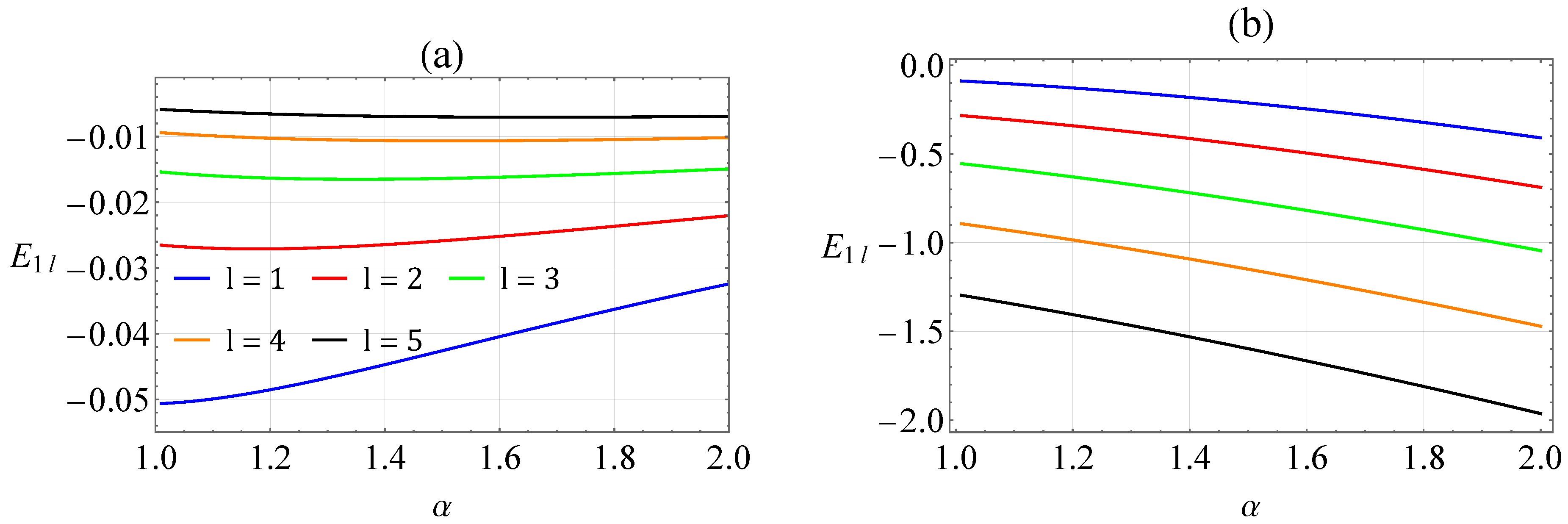
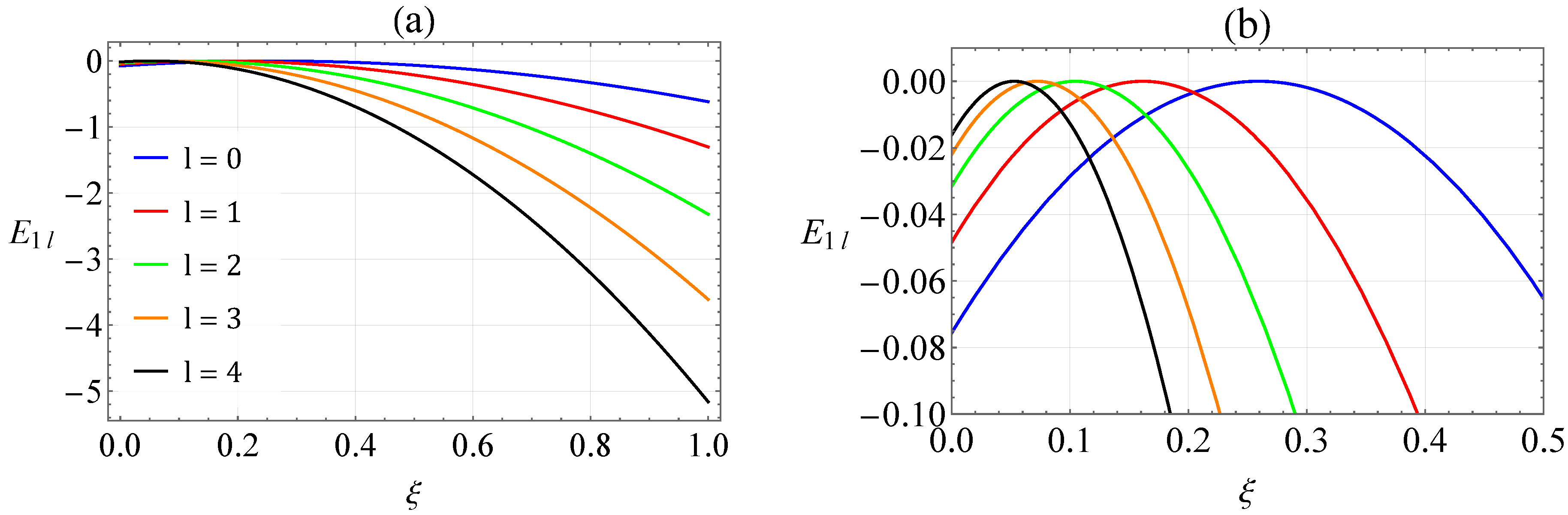
4. Analysis of Bound States

Similarly to the Coulomb potential, the Hulthén potential also admits bound state solutions. The bound state energies can be found from the S-matrix. According to general scattering theory, the poles of the S-matrix in the upper half of the complex plane are associated with the bound state energies. Using the result for the phase shift (40), the S-matrix can be written as
S = e 2 i δ l ,
= e i π + 1 e 2 i   arg Γ 2 i κ e 2 i   arg Γ d + i κ Δ e 2 i   arg Γ d + i κ + Δ .
The poles of the S-matrix are given by the poles of the gamma functions  Γ d + i κ Δ and  Γ d + i κ + Δ in Equation (40). However, we must remember that the function  Γ z has poles at  z = n , where n is a non-negative integer. Thus, analyzing the poles of  Γ d + i κ Δ , we obtain
d + i κ Δ = n .
Using the parameters given in Equation (24), we find
d + i 2 M E n l α ξ 2 2 M E n l 2 α 2 ξ 2 = n .
Finally, solving Equation (44) for  E n l , we obtain the energy eigenvalues
E n l = ( d + n ) 2 ( d + n + ) 2 β ( d + n ) 2 , with β = 8 M α 2 2 ξ 2 .
These energies can also be obtained by solving Equation (19) for bound states. We achieve this by solving Equation (19) via the Frobenius method. We use solutions of the form
u y = y γ 1 y ν h y ,
where  ν and  γ are arbitrary constants to be determined and  h ( y ) is an unknown function. Note that the solution (46) is finite at regular singular points  y = 0 y = 1 , and  y = . Substituting this solution into Equation (19), we find the differential equation
h y + 2 γ 1 + 2 γ + 2 ν y y 1 y h y + ν 2 κ b 2 1 y 2 h y + 2 2 γ ν γ 2 y 1 y h y + γ γ 1 λ 2 y 2 1 y h y = 0 ,
where  κ b = k b / ξ k b = 2 M E n l / α > 0 , with “ b ” labeling bound states. The parameters  ν and  γ are determined by canceling out the coefficients
ν 2 κ b 2 = 0 ,
γ γ 1 λ 2 = 0 ,
from which, we find
ν 1 = + κ b or ν 2 = κ b
and
γ 1 = d or γ 2 = 1 d ,
respectively. For bound state solutions, we must choose  ν 1 and  γ 1 above, which leads to the equation
y 1 y h y + ζ 3 1 + ζ 1 + ζ 2 y h y ζ 1 ζ 2 h y = 0 ,
where
ζ 1 = γ 1 + ν 1 + 2 + ν 1 2 ,
ζ 2 = γ 1 + ν 1 2 + ν 1 2 ,
ζ 3 = 2 γ 1 .
Equation (52) is a hypergeometric differential equation. It is known that the singular points of this equation are regular. Therefore, we can assume series solutions around  y = 0 of the form
h y = s = 0 a s y s + c , with a 0 0 .
By substituting the solution (56) into the differential Equation (52), we obtain the indicial equation
a 0 c c 1 + ζ 3 c = 0 ,
whose roots are
c 1 = 0 ,
c 2 = 1 ζ 3 .
and the recurrence relation
a s + 1 = s + c s + c + ζ 1 + ζ 2 + ζ 1 ζ 2 s + c + 1 s + c + ζ 3 a s , for s 0 .
The general solution of (52) is written as
h y = A h 1 y + B h 2 y ,
where A and B are, respectively, the coefficients of the regular and irregular solutions at the origin, with
h 1 y = s = 0 ζ 1 s ζ 2 s 1 s ζ 3 s y s = 2 F 1 ζ 1 , ζ 2 , ζ 3 ; y
and
h 2 y = y 1 ζ 3 s = 0 ζ 1 + 1 ζ 3 s ζ 2 + 1 ζ 3 s 2 ζ 3 s 1 s y s ,
= y 1 ζ 3 2 F 1 ζ 1 + 1 ζ 3 , ζ 2 + 1 ζ 3 , 2 ζ 3 ; y .
The solution (46) is given by
u y = A y d 1 y κ b 2 F 1 ζ 1 , ζ 2 , 2 d ; y + B y 1 d 1 y κ b 2 F 1 ζ 1 + 1 2 d , ζ 2 + 1 2 d , 2 2 d ; y
Since  ζ 3 is not an integer and  u ( y ) = 0 at  y = 0 (or  r ), we shall take  B = 0 . Thus, the relevant solution is
u y = C n l y d 1 y κ b 2 F 1 ζ 1 , ζ 2 , 2 d ; y ,
where  C n l is the normalization constant. To obtain bound states energies, we must require that the series  2 F 1 ζ 1 , ζ 2 , 2 d ; y terminates, resulting in a polynomial of degree n. This means that, in the recurrence relation (60), we must impose that  a n + 1 = 0 , which leads to (with  c 1 = 0 )
n n + ζ 1 + ζ 2 + ζ 1 ζ 2 = 0
or
2 n κ b + d 2 2 + 2 d κ b + 2 d n + n 2 = 0 ,
which, solved for  κ b , provides
κ b = 2 d + n 2 2 n + d > 0 , with n + d 0 .
Using the relation
κ b = 2 M E n l 2 α 2 ξ 2 > 0 ,
in Equation (69), and solving the resulting equation for  E n l , we obtain
E n l = ( d + n ) 2 ( d + n + ) 2 β ( d + n ) 2 , with β = 8 M α 2 2 ξ 2 ,
which is just Equation (45). To ensure the validity of the relation (70), we must require in Equation (69) that
2 > d + n 2 ,
which gives the upper values for n
n < d , with d R R
or, more explicitly,
n < 2 M 2 α 2 ξ Z e 2 K α 1 2 + 1 2 1 + 4 l l + 1 α 2 .
Equation (74) establishes a condition for the occurrence of bound states and, in addition, determines the range for the quantum number n where such states must appear. It should be emphasized that the energies (71) could be obtained directly by substituting  κ i k b in Equation (21). This leads us to the solution (66). The characteristics of the hypergeometric function are well known. As mentioned above, when  ζ 1 = n , with  n = 0 ,   1 ,   2 ,   , and  ζ 3 0 ,   1 ,   2 ,   , the function  2 F 1 ( ζ 1 ,   ζ 2 ,   ζ 3 ;   y ) becomes a polynomial. In this way, the wave function for bound states (as a function of r) reads
u r = C n l 1 e ξ r d e k b r 2 F 1 n , d + κ b 2 + κ b 2 , 2 d ; 1 e ξ r ,
and the expression for the bound state energies can be found in the condition
d + κ b + 2 + κ b 2 = n ,
which, solved for  E n l , leads us again to Equation (45), which, written in its explicit form, reads
E n l = α 2 2 ξ 2 8 M 2 M ξ 2 α 2 ξ 2 Z e 2 K α n + 4 l l + 1 + α 2 2 α + 1 2 n + 4 l l + 1 + α 2 2 α + 1 2 2 .
It can be verified that, for  ξ 0 and keeping the other parameters fixed in Equation (77),  E n l assumes finite values. In Table 1, we show some energy values for  α = 0.7 and different values of l.
It is important to mention that, for  Z e 2 = 0 (absence of the Hulthén potential), the system admits bound states only for  K ( α ) < 0 , i.e., only for the attractive electrostatic self- interaction. However, with the presence of the Hulthén potential, the system also admits bound states for  K ( α ) > 0 . Indeed, this is evidenced in Figure 1 and Figure 2, where the result of the superposition between the potentials  V H r and  V S I r is shown more explicitly. Therefore, bound states are possible only when  V H r V S I r < 0 .
We can study the energies (77) by sketching them as a function of the parameters involved. In all of the energy plots that we illustrate here, we choose, for convenience, to analyze the state with  n = 1 and use  = 1 M = 1 Z = 1 , and  e = 1 . In Figure 5, we plot the energy levels with  n = 1 for different values of l. We can see that  | E 10 | > | E 11 | > | E 12 | following the order of the  α values considered. We also see that the separation between the energy levels with  l = 0 corresponding to a given value of  α is greater than the separation between the energy levels with  l > 0 . For  l > 2 , we observe an inversion between the energy levels with a given value of  α when we compare them with the energy levels with  l < 2 . In this case,  | E 1 l | increases for  l > 2 .
Figure 6 shows plots of energy levels as a function of  α for  n = 1 and two different values of  ξ . Since the parameter  ξ refers to the screening parameter of the Hulthén potential, it must control the profile of these energy levels for some particular choice of the other parameters. As can be noticed,  ξ = 0.01 (Figure 6a and  ξ = 0.5 (Figure 6b) produce different plots, which correspond to distinct physical situations. In the case shown in Figure 6a, we see that, for values of  α in the range of 1.1 to 1.4, there is a decreasing tendency followed by an increase in  | E 1 l | . For  α > 1.4 , we see that  | E 1 l | decreases. On the other hand, Figure 6b reveals that  | E 1 l | increases as  α is increased.
We also investigate how the energy levels are modified by considering different choices for the parameter  ξ . In Figure 7, we plot the energy levels  E 1 l as a function of  ξ for the particular case when  α = 1.5 . As we can see, there is a range of  ξ where  | E 1 l | decreases, whereas, for the other values,  | E 1 l | increases. For increasing values of l | E 1 l | also increases (see, e.g., the energy curve with  l = 4 (solid black curve) in Figure 7a). The various energy profiles illustrated in Figure 5, Figure 6 and Figure 7 can be more easily interpreted when we make a reading of Figure 1 and Figure 2. The energy intervals where  | E 1 | becomes small correspond precisely to the localized regions where a potential well begins to emerge.  | E 1 | can increase or decrease by adjusting the parameters involved.
The energy (77) can be compared with other models in the literature. For example, if we take  α = 1 , we obtain the energies
E n l = 2 ξ 2 2 M 2 M Z e 2 2 ξ 2 n + l + 1 n + l + 1 2 2 .
Moreover, by making the changes  ξ = δ and  M = μ in Equation (78), we find exactly the expression (24) of Reference [72], which also coincides with Equation (32) of Reference [85].

5. Conclusions

In the present manuscript, we investigated the problem of the quantum motion of an electron in the presence of the Hulthén potential in the global monopole spacetime. Due to the existence of the global monopole background, it is necessary to consider the arising of a self-interaction potential. Under such conditions, we started from the Schrödinger equation with vector coupling in spherical coordinates. Then, we obtained the corresponding radial equation through the standard procedure in the literature. By analyzing several profiles of the effective potential, we verified that the problem can be solved for both bound and scattering states. We confirmed this by sketching profiles of the effective potential as a function of r for different choices of the  α parameter and considering some particular values for the parameter  ξ . We used the exponential function transformation approach and an approximation for the centrifugal potential to transform the radial equation coming from the Schrödinger equation into a differential equation of the hypergeometric type. We solved this equation for scattering states and found an expression for the phase shift. We adopted the following procedure to find an expression for the bound state energies: we first obtained the S-matrix. Then, we analyzed its poles. We examined the profile of energies considering the situation where the self-interaction potential is attractive and repulsive. Through some sketches, we showed that both this potential and the  α parameter could modify the bound state energies. We also investigated the probability density function and its dependence on the parameters  α ξ , and the quantum number n. Alternatively, we also solved the problem for bound states using the Frobenius method and confirmed that the bound state energies and wave functions are the same as those already obtained. The justification for using the Frobenius method is that it provides us with an expression that establishes a condition for the occurrence of bound states (Equation (74)).

Author Contributions

S.S.A.: software, supervision, writing—review and editing; M.M.C.: conceptualization, supervision, writing—original draft preparation, writing—review and editing; H.H.: methodology, software, supervision, writing—original draft preparation, writing—review and editing; E.O.S.: conceptualization, methodology, software, supervision, writing—original draft preparation, writing—review and editing, project administration. All authors have read and agreed to the published version of the manuscript.

Funding

Fundação de Amparo à Pesquisa e ao Desenvolvimento Científico e Tecnológico do Maranhão: PRONEM-01852/14 and UNIVERSAL-06395/22; National Council for Scientific and Technological Development: 306308/2022-3; Coordenação de Aperfeicoamento de Pessoal de Nível Superior: 88887.358036/2019-00 and Finance Code 001.

Data Availability Statement

Not applicable.

Acknowledgments

This work was partially supported by the Brazilian agencies CAPES, CNPq, and FAPEMA. E. O. Silva acknowledges CNPq Grant 306308/2022-3, FAPEMA Grants PRONEM-01852/14 and UNIVERSAL-06395/22. M. M. Cunha acknowledges CAPES Grant 88887.358036/2019-00. This study was financed in part by the Coordenação de Aperfeiçoamento de Pessoal de Nível Superior—Brasil (CAPES)—Finance Code 001.

Conflicts of Interest

The authors declare no conflict of interest.

References

  1. Suzko, A.; Velicheva, E. Exactly Solvable Models for the Generalized Schrödinger Equation. In Mathematical Modeling and Computational Science; Adam, G., Buša, J., Hnatič, M., Eds.; Springer: Berlin/Heidelberg, Germany, 2012; pp. 182–188. [Google Scholar]
  2. Griffiths, D.J. Introduction to Quantum Mechanics, 2nd ed.; Addison-Wesley: Boston, MA, USA, 2005. [Google Scholar]
  3. Davies, B.; Delves, L.M. An Exactly Soluble Two-body Problem with Non-central Forces. Aust. J. Phys. 1963, 16, 311–313. [Google Scholar] [CrossRef] [Green Version]
  4. Karayer, H.; Demirhan, D. Exact analytical solution of Schrödinger equation for a generalized noncentral potential. Eur. Phys. J. Plus 2022, 137, 527. [Google Scholar] [CrossRef]
  5. Wang, X.H.; Chen, C.Y.; You, Y.; Lu, F.L.; Sun, D.S.; Dong, S.H. Exact solutions of the Schrödinger equation for a class of hyperbolic potential well. Chin. Phys. B 2022, 31, 040301. [Google Scholar] [CrossRef]
  6. López-Villanueva, J.A.; Melchor, I.; Cartujo, P.; Carceller, J.E. Modified Schrödinger equation including nonparabolicity for the study of a two-dimensional electron gas. Phys. Rev. B 1993, 48, 1626–1631. [Google Scholar] [CrossRef] [PubMed]
  7. El-Nabulsi, R.A. Quantum dynamics in low-dimensional systems with position-dependent mass and product-like fractal geometry. Phys. E Low-Dimens. Syst. Nanostruct. 2021, 134, 114827. [Google Scholar] [CrossRef]
  8. Biswas, D.; Ghosh, S. Quantum mechanics of a particle on a torus knot: Curvature and torsion effects. Europhys. Lett. 2020, 132, 10004. [Google Scholar] [CrossRef]
  9. Vilenkin, A.; Shellard, E.P.S. Cosmic Strings and Other Topological Defects; Cambridge University Press: Canbridge, UK, 2000. [Google Scholar]
  10. Durrer, R.; Kunz, M.; Melchiorri, A. Cosmic structure formation with topological defects. Phys. Rep. 2002, 364, 1–81. [Google Scholar] [CrossRef] [Green Version]
  11. Ma, L.; Zeng, X.C. Unravelling the Role of Topological Defects on Catalytic Unzipping of Single-Walled Carbon Nanotubes by Single Transition Metal Atom. J. Phys. Chem. Lett. 2018, 9, 6801–6807. [Google Scholar] [CrossRef] [PubMed]
  12. Jagodzinski, H. Points, lines and walls in liquid crystals, magnetic systems and various ordered media by M. Kléman. Acta Crystallogr. Sect. A 1984, 40, 309–310. [Google Scholar] [CrossRef] [Green Version]
  13. Vilenkin, A. Gravitational field of vacuum domain walls and strings. Phys. Rev. D 1981, 23, 852–857. [Google Scholar] [CrossRef]
  14. De A Marques, G.; Bezerra, V.B. Non-relativistic quantum systems on topological defects spacetimes. Class. Quantum Gravity 2002, 19, 985–995. [Google Scholar] [CrossRef]
  15. Katanaev, K.O. Geometric theory of defects. Physics-Uspekhi 2005, 48, 675. [Google Scholar] [CrossRef] [Green Version]
  16. Katanaev, M.O.; Volovich, I.V. Theory of defects in solids and three-dimensional gravity. Ann. Phys. 1992, 216, 1–28. [Google Scholar] [CrossRef]
  17. Ahmed, F. Effects of rotating frames of reference and Cornell-type potential on modified quantum oscillator field in magnetic cosmic string space–time. Int. J. Mod. Phys. A 2022, 37, 2250122. [Google Scholar] [CrossRef]
  18. Yang, Y.; Jing, J.; Tian, Z. Probing cosmic string spacetime through parameter estimation. Eur. Phys. J. C 2022, 82, 688. [Google Scholar] [CrossRef]
  19. Edet, C.; Nwbabuzor, P.; Ettah, E.; Duque, C.; Ali, N.; Ikot, A.; Mahmoud, S.; Asjad, M. Magneto-transport and thermal properties of the Yukawa potential in cosmic string space-time. Results Phys. 2022, 39, 105749. [Google Scholar] [CrossRef]
  20. Chen, H.; Long, Z.W.; Long, C.Y.; Zare, S.; Hassanabadi, H. The influence of Aharonov–Casher effect on the generalized Dirac oscillator in the cosmic string space-time. Int. J. Geom. Methods Mod. Phys. 2022, 19, 2250133. [Google Scholar] [CrossRef]
  21. Zhou, R.; Bian, L. Gravitational waves from cosmic strings after a first-order phase transition. Chin. Phys. C 2022, 46, 043104. [Google Scholar] [CrossRef]
  22. Mustafa, O. PDM Klein–Gordon oscillators in cosmic string spacetime in magnetic and Aharonov–Bohm flux fields within the Kaluza–Klein theory. Ann. Phys. 2022, 440, 168857. [Google Scholar] [CrossRef]
  23. Cuzinatto, R.R.; de Montigny, M.; Pompeia, P.J. Non-commutativity and non-inertial effects on a scalar field in a cosmic string space-time: I. Klein–Gordon oscillator. Class. Quantum Gravity 2022, 39, 075006. [Google Scholar] [CrossRef]
  24. Cuzinatto, R.R.; de Montigny, M.; Pompeia, P.J. Non-commutativity and non-inertial effects on a scalar field in a cosmic string space-time: II. Spin-zero Duffin–Kemmer–Petiau-like oscillator. Class. Quantum Gravity 2022, 39, 075007. [Google Scholar] [CrossRef]
  25. Ahmed, F. Generalized Klein–Gordon oscillator with a uniform magnetic field under the influence of Coulomb-type potentials in cosmic string space–time and Aharonov–Bohm effect. Can. J. Phys. 2021, 99, 496–500. [Google Scholar] [CrossRef]
  26. Ahmed, F. Effects of uniform rotation and electromagnetic potential on the modified Klein–Gordon oscillator in a cosmic string space-time. Int. J. Geom. Methods Mod. Phys. 2021, 18, 2150187. [Google Scholar] [CrossRef]
  27. Silva, M.; Mohammadi, A. Scattering cross-section in gravitating cosmic string spacetimes. Class. Quantum Gravity 2021, 38, 205006. [Google Scholar] [CrossRef]
  28. Guvendi, A.; Hassanabadi, H. Relativistic Vector Bosons with Non-minimal Coupling in the Spinning Cosmic String Spacetime. Few-Body Syst. 2021, 62, 57. [Google Scholar] [CrossRef]
  29. Yang, Y.; Hassanabadi, H.; Chen, H.; Long, Z.W. DKP oscillator in the presence of a spinning cosmic string. Int. J. Mod. Phys. E 2021, 30, 2150050. [Google Scholar] [CrossRef]
  30. Ahmed, F. Spin-0 scalar particle interacts with scalar potential in the presence of magnetic field and quantum flux under the effects of KKT in 5D cosmic string spacetime. Mod. Phys. Lett. A 2021, 36, 2150004. [Google Scholar] [CrossRef]
  31. Cunha, M.M.; Silva, E.O. Self-Adjoint Extension Approach to Motion of Spin-1/2 Particle in the Presence of External Magnetic Fields in the Spinning Cosmic String Spacetime. Universe 2020, 6, 203. [Google Scholar] [CrossRef]
  32. Cunha, M.M.; Dias, H.S.; Silva, E.O. Dirac oscillator in a spinning cosmic string spacetime in external magnetic fields: Investigation of the energy spectrum and the connection with condensed matter physics. Phys. Rev. D 2020, 102, 105020. [Google Scholar] [CrossRef]
  33. Hosseinpour, M.; Hassanabadi, H. Scattering states of Dirac equation in the presence of cosmic string for Coulomb interaction. Int. J. Mod. Phys. A 2015, 30, 1550124. [Google Scholar] [CrossRef]
  34. Sun, X.Q.; Zhu, P.; Hughes, T.L. Geometric Response and Disclination-Induced Skin Effects in Non-Hermitian Systems. Phys. Rev. Lett. 2021, 127, 066401. [Google Scholar] [CrossRef]
  35. Oliveira, J.; Garcia, G.; Porfírio, P.; Furtado, C. Graphene-based topological insulator in the presence of a disclination submitted to a uniform magnetic field. Ann. Phys. 2021, 425, 168384. [Google Scholar] [CrossRef]
  36. Zare, S.; Hassanabadi, H.; de Montigny, M. Nonrelativistic particles in the presence of a Cariñena–Perelomov–Rañada–Santander oscillator and a disclination. Int. J. Mod. Phys. A 2020, 35, 2050071. [Google Scholar] [CrossRef]
  37. Belouad, A.; Jellal, A.; Bahlouli, H. Electronic properties of graphene quantum ring with wedge disclination. Eur. Phys. J. B 2021, 94, 75. [Google Scholar] [CrossRef]
  38. Jiang, J.; Ranabhat, K.; Wang, X.; Rich, H.; Zhang, R.; Peng, C. Active transformations of topological structures in light-driven nematic disclination networks. Proc. Natl. Acad. Sci. USA 2022, 119, e2122226119. [Google Scholar] [CrossRef] [PubMed]
  39. Monderkamp, P.A.; Wittmann, R.; te Vrugt, M.; Voigt, A.; Wittkowski, R.; Löwen, H. Topological fine structure of smectic grain boundaries and tetratic disclination lines within three-dimensional smectic liquid crystals. Phys. Chem. Chem. Phys. 2022, 24, 15691–15704. [Google Scholar] [CrossRef] [PubMed]
  40. Bakke, K. Topological effects of a disclination on quantum revivals. Int. J. Mod. Phys. A 2022, 37, 2250046. [Google Scholar] [CrossRef]
  41. Pandey, A.; Singh, M.; Gupta, A. Positive disclination in a thin elastic sheet with boundary. Phys. Rev. E 2021, 104, 065002. [Google Scholar] [CrossRef]
  42. Kleinert, H. Gauge Fields in Condensed Matter; World Scientific: Singapore, 1989. [Google Scholar] [CrossRef]
  43. Su, W.P.; Schrieffer, J.R.; Heeger, A.J. Soliton excitations in polyacetylene. Phys. Rev. B 1980, 22, 2099–2111. [Google Scholar] [CrossRef]
  44. Kleman, M.; Friedel, J. Disclinations, dislocations, and continuous defects: A reappraisal. Rev. Mod. Phys. 2008, 80, 61–115. [Google Scholar] [CrossRef] [Green Version]
  45. Barriola, M.; Vilenkin, A. Gravitational field of a global monopole. Phys. Rev. Lett. 1989, 63, 341–343. [Google Scholar] [CrossRef] [PubMed]
  46. Kaur, L.; Wazwaz, A.M. Einstein’s vacuum field equation: Painlevé analysis and Lie symmetries. Waves Random Complex Media 2021, 31, 199–206. [Google Scholar] [CrossRef]
  47. Kaur, L.; Gupta, R.K. On certain new exact solutions of the Einstein equations for axisymmetric rotating fields. Chin. Phys. B 2013, 22, 100203. [Google Scholar] [CrossRef]
  48. Kaur, L.; Gupta, R.K. On symmetries and exact solutions of the Einstein–Maxwell field equations via the symmetry approach. Phys. Scr. 2013, 87, 035003. [Google Scholar] [CrossRef]
  49. Ali, M.S.; Bhattacharya, S. Vacuum polarization of Dirac fermions in the cosmological de Sitter global monopole spacetime. Phys. Rev. D 2022, 105, 085006. [Google Scholar] [CrossRef]
  50. Grats, Y.V.; Spirin, P.A. Vacuum polarization in the field of a multidimensional global monopole. J. Exp. Theor. Phys. 2016, 123, 807–813. [Google Scholar] [CrossRef]
  51. Barroso, V.S.; Pitelli, J.P.M. Vacuum fluctuations and boundary conditions in a global monopole. Phys. Rev. D 2018, 98, 065009. [Google Scholar] [CrossRef] [Green Version]
  52. Ahmed, F. Relativistic motions of spin-zero quantum oscillator field in a global monopole space-time with external potential and AB-effect. Sci. Rep. 2022, 12, 8794. [Google Scholar] [CrossRef]
  53. De Montigny, M.; Pinfold, J.; Zare, S.; Hassanabadi, H. Klein–Gordon oscillator in a global monopole space–time with rainbow gravity. Eur. Phys. J. Plus 2021, 137, 54. [Google Scholar] [CrossRef]
  54. Bragança, E.A.F.; Vitória, R.L.L.; Belich, H.; de Mello, E.R.B. Relativistic quantum oscillators in the global monopole spacetime. Eur. Phys. J. C 2020, 80, 206. [Google Scholar] [CrossRef] [Green Version]
  55. Anacleto, M.; Brito, F.; Ferreira, S.; Passos, E. Absorption and scattering of a black hole with a global monopole in f(R) gravity. Phys. Lett. B 2019, 788, 231–237. [Google Scholar] [CrossRef]
  56. Pu, J.; Han, Y. On Hawking Radiation via Tunneling from the Reissner-Nordström-de Sitter Black Hole with a Global Monopole. Int. J. Theor. Phys. 2017, 56, 2061–2070. [Google Scholar] [CrossRef]
  57. Shao, J.Z.; Wang, Y.J. Scattering and absorption of particles by a black hole involving a global monopole. Chin. Phys. B 2012, 21, 040404. [Google Scholar] [CrossRef]
  58. Ita, B.I.; Louis, H.; Ubana, E.I.; Ekuri, P.E.; Leonard, C.U.; Nzeata, N.I. Evaluation of the bound state energies of some diatomic molecules from the approximate solutions of the Schrodinger equation with Eckart plus inversely quadratic Yukawa potential. J. Mol. Model. 2020, 26, 349. [Google Scholar] [CrossRef]
  59. Onyenegecha, C.P.; Ukewuihe, U.M.; Opara, A.I.; Agbakwuru, C.B.; Okereke, C.J.; Ugochukwu, N.R.; Okolie, S.A.; Njoku, I.J. Approximate solutions of Schrödinger equation for the Hua plus modified Eckart potential with the centrifugal term. Eur. Phys. J. Plus 2020, 135, 571. [Google Scholar] [CrossRef]
  60. Louis, H.; Ita, B.I.; Nzeata, N.I. Approximate solution of the Schrödinger equation with Manning-Rosen plus Hellmann potential and its thermodynamic properties using the proper quantization rule. Eur. Phys. J. Plus 2019, 134, 315. [Google Scholar] [CrossRef]
  61. Oyewumi, K.; Falaye, B.; Onate, C.; Oluwadare, O.; Yahya, W. Thermodynamic properties and the approximate solutions of the Schrödinger equation with the shifted Deng–Fan potential model. Mol. Phys. 2014, 112, 127–141. [Google Scholar] [CrossRef]
  62. Bayrak, O.; Boztosun, I. Bound state solutions of the Hulthén potential by using the asymptotic iteration method. Phys. Scr. 2007, 76, 92–96. [Google Scholar] [CrossRef]
  63. Agboola, D. The Hulthén potential in D-dimensions. Phys. Scr. 2009, 80, 065304. [Google Scholar] [CrossRef] [Green Version]
  64. Saad, N. The Klein–Gordon equation with a generalized Hulthén potential in D-dimensions. Phys. Scr. 2007, 76, 623–627. [Google Scholar] [CrossRef]
  65. Peng, X.L.; Liu, J.Y.; Jia, C.S. Approximation solution of the Dirac equation with position-dependent mass for the generalized Hulthén potential. Phys. Lett. A 2006, 352, 478–483. [Google Scholar] [CrossRef]
  66. Hosseinpour, M.; Andrade, F.M.; Silva, E.O.; Hassanabadi, H. Scattering and bound states for the Hulthén potential in a cosmic string background. Eur. Phys. J. C 2017, 77, 270. [Google Scholar] [CrossRef] [Green Version]
  67. Jusufi, K.; Werner, M.C.; Banerjee, A.; Övgün, A. Light deflection by a rotating global monopole spacetime. Phys. Rev. D 2017, 95, 104012. [Google Scholar] [CrossRef] [Green Version]
  68. Bezerra de Mello, E.R.; Furtado, C. Nonrelativistic scattering problem by a global monopole. Phys. Rev. D 1997, 56, 1345–1348. [Google Scholar] [CrossRef]
  69. Hulthén, L. On the characteristic solutions of the Schrödinger deuteron equation. Ark. Mat. Astron. Fys. A 1942, 28, 5. [Google Scholar]
  70. Qiang, W.C.; Dong, S.H. Analytical approximations to the solutions of the Manning–Rosen potential with centrifugal term. Phys. Lett. A 2007, 368, 13–17. [Google Scholar] [CrossRef]
  71. Chen, C.Y.; Lu, F.L.; Sun, D.S. Approximate analytical solutions of scattering states for Klein-Gordon equation with Hulthén potentials for nonzero angular momentum. Cent. Eur. J. Phys. 2008, 6, 884–890. [Google Scholar] [CrossRef]
  72. Jia, C.S.; Liu, J.Y.; Wang, P.Q. A new approximation scheme for the centrifugal term and the Hulthén potential. Phys. Lett. A 2008, 372, 4779–4782. [Google Scholar] [CrossRef]
  73. Sakurai, J.J. Modern Quantum Mechanics, revised ed.; Addison-Wesley: Boston, MA, USA, 1994. [Google Scholar]
  74. Wei, G.-F.; Chen, W.-L.; Wang, H.-Y.; Li, Y.-Y. The scattering states of the generalized Hulthén potential with an improved new approximate scheme for the centrifugal term. Chin. Phys. B 2009, 18, 3663–3669. [Google Scholar] [CrossRef]
  75. Hassanabadi, H.; Yazarloo, B.H.; Hassanabadi, S.; Zarrinkamar, S. The Semi-Relativistic Scattering States of the Hulthén and Hyperbolic-Type Potentials. Acta Phys. Pol. A 2013, 124, 20–22. [Google Scholar] [CrossRef]
  76. Landau, L.; Lifshitz, E. Quantum Mechanics: Non-Relativistic Theory; Course of Theoretical Physics; Elsevier Science: Amsterdam, The Netherlands, 1981. [Google Scholar]
  77. Greene, R.L.; Aldrich, C. Variational wave functions for a screened Coulomb potential. Phys. Rev. A 1976, 14, 2363–2366. [Google Scholar] [CrossRef]
  78. Adebimpe, O.; Onate, C.; Salawu, S.; Abolanriwa, A.; Lukman, A. Eigensolutions, scattering phase shift and thermodynamic properties of Hulthén-Yukawa potential. Results Phys. 2019, 14, 102409. [Google Scholar] [CrossRef]
  79. Ahmadov, A.; Aslanova, S.; Orujova, M.; Badalov, S.; Dong, S.H. Approximate bound state solutions of the Klein-Gordon equation with the linear combination of Hulthén and Yukawa potentials. Phys. Lett. A 2019, 383, 3010–3017. [Google Scholar] [CrossRef]
  80. Edet, C.O.; Ikot, A.N. Effects of Topological Defect on the Energy Spectra and Thermo-magnetic Properties of CO Diatomic Molecule. J. Low Temp. Phys. 2021, 203, 84–111. [Google Scholar] [CrossRef]
  81. Eshghi, M.; Sever, R.; Ikhdair, S.M. Energy states of the Hulthen plus Coulomb-like potential with position-dependent mass function in external magnetic fields. Chin. Phys. B 2018, 27, 020301. [Google Scholar] [CrossRef] [Green Version]
  82. Aomoto, K.; Kita, M.; Kohno, T.; Iohara, K. Theory of Hypergeometric Functions; Springer Monographs in Mathematics; Springer: Tokyo, Japan, 2011. [Google Scholar]
  83. Abramowitz, M.; Stegun, I.A. Handbook of Mathematical Functions; Dover Publications: New York, NY, USA, 1972. [Google Scholar]
  84. Olver, F.W.J.; Lozier, D.W.; Boisvert, R.F.; Clark, C.W. (Eds.) NIST Handbook of Mathematical Functions; Cambridge University Press: Cambridge, UK, 2010. [Google Scholar]
  85. Bayrak, O.; Kocak, G.; Boztosun, I. Any l-state solutions of the Hulthén potential by the asymptotic iteration method. J. Phys. Math. Gen. 2006, 39, 11521–11529. [Google Scholar] [CrossRef] [Green Version]
Figure 1. Effective potential (Equation (14)) as a function of r for different values of  α < 1 . Four situations involving  ξ and l are considered: (a ξ = 0.1 and  l = 1 , (b ξ = 0.65 and  l = 1 , (c ξ = 0.21 and  l = 2 , and (d ξ = 0.65 and  l = 3 .
Universe 09 00132 g001
Figure 2. Effective potential (Equation (14)) as a function of r for different values of  α > 1 . Four situations involving  ξ and l are considered: (a ξ = 0.1 and  l = 1 , (b ξ = 0.65 and  l = 1 , (c ξ = 0.21 and  l = 2 , and (d ξ = 0.65 and  l = 3 .
Universe 09 00132 g002
Figure 3. The plots of  | u ( r ) | 2 as a function of r for different values of n displayed for (a α = 0.2 ξ = 0.1 , (b α = 0.8 ξ = 0.1 , (c α = 0.2 ξ = 0.65 , and (d α = 0.8 ξ = 0.65 . We use the parameters  = 1 M = 1 e = 1 k = 1 , and  l = 1 .
Universe 09 00132 g003
Figure 4. The plots of  | u ( r ) | 2 as a function of r for different values of n displayed for (a α = 1.2 ξ = 0.1 , (b α = 1.8 ξ = 0.1 , (c α = 1.2 ξ = 0.65 , and (d α = 1.8 ξ = 0.65 . We use the parameters  = 1 M = 1 e = 1 k = 1 , and  l = 1 .
Universe 09 00132 g004
Figure 5. Energy levels (Equation (77)) with  n = 1 as a function of l for  ξ = 0.1 . In (a), we display the energies corresponding to different values of  α > 1 and, in (b), values of  α < 1 . An inversion between the two profiles is observed at  l = 2 .
Universe 09 00132 g005
Figure 6. Energy levels (Equation (77)) with  n = 1 as a function of  α for (a ξ = 0.01 and (b ξ = 0.5 .
Universe 09 00132 g006
Figure 7. Energy levels (Equation (77)) with  n = 1 as a function of  ξ for  α = 1.5 . In (b), we show the range from (a) to  ξ = 0.5 .
Universe 09 00132 g007
Table 1. Energies in the limit  ξ 0 for  n = 1 and different values of l (Equation (77)). We assume that  = 1 , M = 1 , Z = 1 , e = 1 , n = 1 and  α = 0.7 .
  E n , l Values
  E 1 , 1   0.0472842
  E 1 , 2   0.0236029
  E 1 , 3   0.0141781
  E 1 , 4   0.0094620
  E 1 , 5   0.0067639
  E 1 , 6   0.0050758
  E 1 , 7   0.0039496
  E 1 , 8   0.0031608
  E 1 , 9   0.0025868
  E 1 , 10   0.0021561
Disclaimer/Publisher’s Note: The statements, opinions and data contained in all publications are solely those of the individual author(s) and contributor(s) and not of MDPI and/or the editor(s). MDPI and/or the editor(s) disclaim responsibility for any injury to people or property resulting from any ideas, methods, instructions or products referred to in the content.

