Abstract
Telescopes such as the Large Sky Area Multi-Object Spectroscopic Telescope and the Sloan Digital Sky Survey have produced an extensive collection of spectra, challenging the feasibility of manual classification in terms of accuracy and efficiency. To overcome these limitations, machine learning techniques are increasingly being utilized for automated spectral classification. However, these approaches primarily treat spectra as frequency domain signals, and lack robustness in low signal-to-noise ratio (S/N) scenarios and for small datasets of rare celestial objects. Moreover, they frequently neglect nuanced expert astronomical understanding. In this study, we draw inspiration from the human spectral discrimination process and propose a new model called the Image-EFficientNetV2-Spectrum Convolutional Neural Network (IEF-SCNN). IEF-SCNN combines spectral images using EfficientNetV2 with one-dimensional (1D) spectra through a 1DCNN. This integration effectively incorporates astronomical expertise into the classification process. Specifically, we plot the spectrum as an image and then classify it in a way that incorporates an attention mechanism. This attention mechanism mimics human observation of images for classification, selectively emphasizing relevant information while ignoring irrelevant details. Experimental data demonstrate that IEF-SCNN outperforms existing models in terms of the F1-score and accuracy metrics, particularly for low S/N (<6) data. Using progressive learning and an attention mechanism, the model trained on 12,000 M-class stars with an S/N below 6 achieved an accuracy of 87.38% on a 4000-sample test set. This surpasses traditional models (support vector machine with 83.15% accuracy, random forest with 65.40%, and artificial neural network with 84.40%) and the 1D stellar spectral CNN (85.65% accuracy). This research offers a foundation for the development of innovative methods for the automated identification of specific celestial objects, and can promote the creation of user-friendly software for astronomers who may not have computational expertise.
1. Introduction
In recent decades, astronomical survey telescopes such as the Sloan Digital Sky Survey (SDSS) [1] and the Large Sky Area Multi-Object Spectroscopic Telescope (LAMOST) [2] have amassed a substantial volume of spectral data. This invaluable spectral information has made significant contributions to the advancement of astronomical research. Nonetheless, the task of categorizing this vast array of spectra is formidable and presents a substantial challenge.
The MK classification system [3] is a widely utilized method for categorizing stars based on their temperature and brightness attributes. Initially, this classification relied on human experts who applied their experience and visual analysis. However, manual classification is susceptible to subjective errors and is notably inefficient. Consequently, template matching methods [4,5] were developed as an alternative approach. However, template matching may face performance challenges when handling intricate spectra.
The exponential growth in data samples coupled with advancements in computer hardware has spurred the development of numerous machine learning and deep learning-based methods that can address the challenges involved in spectral classification. Machine learning techniques have found widespread application in this context. For instance, in [6], an artificial neural network (ANN) was employed for spectral classification. In [7], the authors utilized principal component analysis to reduce dimensionality before employing ANN for classification. In cases with a low signal-to-noise ratio (S/N), as described in [8], an ANN was applied to process spectral data. Furthermore, ref. [9] introduced the MKCLASS program, which classifies spectra based on their deviation from the MK standard spectra. The random forest algorithm, as detailed in [10], was employed for stellar spectral classification and feature evaluation. In [11], the authors investigated the application of probabilistic neural networks, support vector machines, and K-means in spectral classification. Finally, ref. [12] proposed an entropy-based approach for classifying unbalanced spectral data. For an in-depth exploration of how machine learning is employed in the classification of astronomical spectra, ref. [13] provides a comprehensive review.
Deep learning techniques have gained traction in spectral classification. For instance, ref. [14] introduced deep neural networks for the prediction of star parameters, while [15] proposed an automated method for classifying stellar spectra in the optical range using convolutional neural networks (CNNs). In [16], the authors introduced a nine-layer one-dimensional stellar spectral CNN (1D SSCNN) architecture for the classification of F, G, and K stellar spectra. In [17], the authors improved CNN performance by incorporating a residual structure and an attention mechanism.
Nevertheless, prior studies have typically involved the extraction of features from raw spectral data (or direct input of raw data) and subsequent construction of classification models using processed data. These approaches primarily rely on statistical knowledge, and do not effectively incorporate the expertise of astronomers.
In this study, we draw inspiration from the process of human spectral discrimination and propose a novel approach to categorizing stellar spectra by treating them as images within the field of computer vision. We suggest that human experts classify spectra by visually examining these spectral “images”, focusing on salient features while disregarding less relevant ones. In our research, we emulate this process by plotting spectra into image representations and incorporating an attention mechanism. Recent advancements in image classification models, including MobileNetV2 [18], ViT [19], and EfficientNetV2 [20], have been noteworthy; in particular, EfficientNetV2 has demonstrated remarkable performance and efficiency, achieving top-1 accuracy on ImageNet ILSVRC2012 and surpassing ViT while training significantly more quickly with equivalent computing resources. Therefore, in light of the substantial volume of astronomical data, we opted to utilize EfficientNetV2 for processing spectral images. Furthermore, we explored a hybrid approach by combining 1D spectral data with the image representations plotted from the spectra. Motivated by this concept, we have devised a model built upon the foundations of EfficientNetV2 and a 1D SSCNN that is able to handle both images and 1D spectral data. In the case of EfficientNetV2, we tailored the attention mechanism and progressive learning components to better suit the characteristics of astronomical data. Simultaneously, for the 1D SSCNN component, we integrated a convolutional structure and employed an attention mechanism to enhance compatibility with EfficientNetV2.
The subsequent sections of this paper are structured as follows. Section 2 introduces the data and describes the preprocessing steps applied to the spectral data obtained from the SDSS database. Section 3 provides an overview of our methodology. Section 4 presents a comparative analysis of the experimental results obtained with our model in relation to other existing models. Section 5 comprises a series of discussions regarding the implications of the experimental findings. Finally, Section 6 concludes the paper and identifies potential areas for further research.
2. Data and Preprocessing
The SDSS represents a notably ambitious and successful survey project that provides access to spectra and deep multicolor images of celestial objects. Spectral data from SDSS DR16 are openly available to the public through the Casjobs server [21],1 enabling users to download data accompanied by relevant labels. In this particular study, we acquired stellar data including five classes: A, F, G, K, and M, as well as five subclasses within the M-type stars spanning the range from 0 to 4. These two sets of classifications correspond to two distinct categorization tasks. The initial step in data preprocessing entails the normalization of the data. To accomplish this, the flux values must be transformed into the range of 0 to 1 following the procedure outlined below:
where f represents the flux and and denote the minimum and maximum flux values, respectively.
To maintain a consistent input format, we confined the wavelength range in the normalized data to span from 4000 Å to 9000 Å, resulting in a data size of 1 × 3522. As our model incorporates images, it is crucial to visualize the preprocessed data in the form of images as well. In the domain of deep learning, the resolution of an image can exert a significant influence on training results. In theory, higher-resolution images can encapsulate more information and potentially yield superior training results. Nevertheless, larger images may introduce challenges such as overfitting and protracted training times. Considering that EfficientNetV2 employs a resolution of 380 × 380 [20], we maintained this resolution in order to ensure consistency and avoid compromising performance. During the training phase, we employed a resolution of 300 × 300 to expedite the training process, with a transition to 380 × 380 during testing, aligning with the specifications outlined in the original EfficientNetV2 papers.
In addition to image resolution, the line width of the drawn spectrum plays a crucial role in influencing the experimental results. The term “line width” pertains to the thickness of the lines, and is measured in pixels. We utilized the matplotlib plot function2 to plot these spectral images; line width serves as one of the optional parameters within this function. While a larger line width facilitate improved information acquisition, it may sacrifice finer details; on the other hand, a narrower line width capture more complex details at the expense of slower convergence during training. Considering that EfficientNetV2 requires input data with three channels corresponding to RGB colors, and our spectral images inherently possess only one color, we addressed this disparity by generating three distinct images, each with a different line width, to populate the three color channels. This approach is elucidated in Figure 1, where the model simultaneously processes three distinct images of a single spectrum.
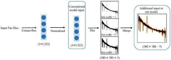
Figure 1.
Spectral preprocessing: first, the spectrum is extracted, cropped, and normalized to obtain a 1 × 3522 vector. Then, this vector is used to plot three single-channel images, each with a different line width that represents the width of the spectral lines in the image. The x-axis represents the wavelength, while the y-axis represents the relative flux. Finally, these three single-channel images are merged into a single three-channel image, with each channel corresponding to one of the three images.
Figure 1 illustrates that the conventional model accepts the normalized 1D data obtained by extracting the spectral flux and resizing it to a consistent dimension as input. In this study, the model endeavors to enhance its classification capacity by incorporating the spectral image generated through spectral plotting alongside the 1D spectral data.
3. Method
In this study, we introduce an innovative model referred to as IEF-S CNN (Image EfficientNetV2-Spectrum) that seamlessly integrates spectral images and 1D spectral data to facilitate the classification process. The network architecture of EfficientNetV2 is harnessed to extract salient features from the image component. Furthermore, specialized attention and progressive learning modules are enhanced to cater specifically to the characteristics of astronomical spectral data. To capture features from the 1D spectral component, we devised a structured 1D convolutional neural network (1DCNN). Ultimately, the features extracted from both the images and the 1D spectral data are synergistically amalgamated to serve the classification objective.
3.1. EfficientNetV2
EfficientNet [22], proposed by Google in 2019, represents an advanced network architecture that has demonstrated remarkable performance in image classification. The success of EfficientNet can be attributed to two pivotal factors. First, Google harnessed its formidable computing power to conduct a thorough neural network search, culminating in the discovery of an enhanced network structure. Second, while traditional CNN models typically rely on augmenting the size of the convolutional kernel, the depth of the network, and the input resolution individually to improve performance, EfficientNet adopts a holistic approach by optimizing all three aspects concurrently, leading to superior results.
In this study, we employed EfficientNetV2, an improved iteration of EfficientNet [20], which introduces two notable enhancements. First, it accelerates the training speed of shallower networks. Second, it introduces a progressive learning technique that dynamically adjusts the regularization method (e.g., dropout) based on the training image size. This approach expedites the training process and elevates accuracy. In comparison to its predecessor, EfficientNetV2 achieves an eleven-fold increase in training speed while reducing the number of parameters to 1/6.8. EfficientNetV2 comprises a combination of MBConv [18] and FusedMBConv blocks. The fundamental element within MBConv is the mobile inverted bottleneck, which incorporates an attention mechanism. It comprises two standard convolutional layers, namely, a depthwise convolutional layer and a squeeze–excitation (SE) [23] attention mechanism. FusedMBConv addresses the inefficiency of the depthwise convolution layer in MBConv by replacing the previous normal convolution and depthwise convolution layers with a single normal convolution, facilitating hardware acceleration.
EfficientNetV2 models of various sizes have been developed and tailored to different tasks. In this specific study, recognizing the relatively lower complexity of spectral images compared to natural images, we chose to utilize the smallest model from the EfficientNetV2 family, EfficientNetV2-S.
3.2. Optimization of the Attention Mechanism
The behavior exhibited by experts who focus on specific features of the spectrum aligns with the concept of the attention mechanism in deep learning. The squeeze–excitation (SE) attention mechanism is employed by EfficientNetV2. However, recognizing the critical role played by the attention mechanism, we opted to replace the SE attention mechanism with two alternative attention mechanisms for the purpose of comparative experiments: efficient channel attention (ECA) [24] and convolutional block attention module (CBAM) [25].
The SE attention mechanism centers its attention on the interplay between different channels. Following a global pooling operation and two fully connected layers, the model discerns the significance of various channels. Nevertheless, the SE attention mechanism compresses the input feature map, leading to a reduction in dimensionality, which can impede the model’s capacity to learn dependencies between channels. In contrast, the ECA attention mechanism bypasses dimensional reduction and adaptively captures local cross-channel interactions through the use of 1D convolution, facilitating the extraction of interchannel dependencies. The size of the 1D convolution kernel, denoted as k, represents a hyperparameter that is varied according to the number of channels, denoted as C. To address this variability, ECA proposes an adaptive approach to determine the optimal size for the 1D convolution kernel.
The calculation of the convolution kernel k is depicted in the following equation, with set to 2 and b set to 1. It is noteworthy that the ECA attention mechanism is conceptually and operationally simpler than the SE attention mechanism, exerting a negligible effect on network processing speed.
In comparison to the SE and ECA attention mechanisms, CBAM is a module that amalgamates both spatial and channel information. In theory, employing CBAM may yield superior experimental results, although it necessitates a greater computational effort. In this study, considering their significance in our research, we included all three attention mechanisms in the experimental phase to facilitate a thorough comparison and evaluation.
3.3. 1DCNN
The structure of the 1DCNN designed in this study is visually presented in Figure 2. It includes four convolutional units along with the ECA (efficient channel attention) mechanism. Additionally, there are flattened and fully connected layers that produce 1 × 1280 features. The 1DCNN effectively extracts features in 1280 dimensions by progressively expanding the number of channels using these four convolutional units. These extracted features undergo compression within the network through a maximum pooling layer. Subsequently, the flattened and fully connected layers convert these compressed features into 1280-dimensional representations. To enhance the feature extraction process, two ECA attention mechanism modules were integrated into the convolutional process.
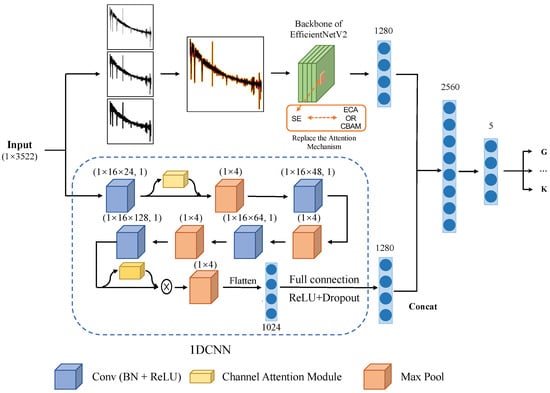
Figure 2.
The entire model structure can be divided into two parts: first, the spectrum is represented as an image and the features are extracted using EfficientNetV2; second, the features of the spectrum are then extracted using 1DCNN. Afterwards, the extracted features from both parts are concatenated and fed into a fully connected layer and softmax function to obtain the classification results.
Each convolutional unit within the 1DCNN consists of four essential components: a convolutional layer, batch normalization [26], rectified linear unit (ReLU) activation function, and dropout layer. The convolutional layer is tasked with feature extraction; in this study, we employed a 1 × 16 convolutional kernel. Batch normalization was incorporated to expedite training and facilitate network convergence, and can additionally help to control gradient issues such as explosion and vanishing gradients while mitigating overfitting.
Following batch normalization, the ReLU activation function is applied. It promotes efficient training via gradient descent and backpropagation. This choice of activation function effectively mitigates problems related to gradient explosion and vanishing gradients. The ReLU activation function is mathematically represented by the following equation, and its calculation process is straightforward, simplifying the overall computational process:
3.4. Overall Model Structure and Training Process
The overall architecture of the model, depicted in Figure 2, can be divided into two components: EfficientNetV2 and 1DCNN. Both components extract features in the form of 1 × 1280 dimensions, which are subsequently concatenated to form 1 × 2560 features. These combined features pass through a fully connected layer, followed by a softmax activation function, resulting in a probability distribution for each category.
All preprocessed spectra, having previously undergone normalization, are represented as 1 × 3522 dimensional data. These normalized spectra serve as the input for the entire model, and training occurs in two parallel aspects:
1. The input data undergo transformation into three 380 × 380 images, each with varying line widths. These three images are then amalgamated into a single image through the RGB channels, collectively serving as input to the EfficientNetV2 backbone. The output of this process yields a 1 × 1280 feature matrix denoted as .
2. The data are directly used as the input of the 1DCNN, and the output is a 1 × 1280 feature matrix denoted as .
The outputs from both parts are concatenated to form . The classification results are obtained after passing through a fully connected layer.
The training of our model is divided into two steps. First, in the initial stage of training, which uses two thirds of the training epoch, the loss for the output results of and is calculated using the cross-entropy loss [27]. The loss is defined in Equations (4) and (5), where C represents the number of classes and is the true label of the data. Second, in the later stage of training, using one third of the training epoch, the cosine similarity between and is calculated in order to facilitate the fusion of the features from both parts ( and ). These two losses are defined in Equations (6) and (7).
In summary, the comprehensive loss calculation for our model is depicted in Equation (8). Following numerous experiments, we determined the hyperparameters , , , and , which we respectively set as {0, 0.2, 0.8, 0} during the initial training phase and {0.2, 0, 0.4, 0.2} during the later stages of training.
3.5. Optimization of Progressive Learning
Progressive learning is a methodology that entails commencing training with low-resolution images during the early stages and gradually increasing the resolution of training images over time. The primary objective of progressive learning is to enhance training speed, although it often comes at the cost of decreased accuracy. To mitigate this decline in accuracy, EfficientNetV2 incorporates adaptive tuning regularization techniques such as dropout to simultaneously improve both training speed and accuracy. Specifically, adaptive tuning regularization is applied when dealing with smaller training image sizes, whereas stronger data augmentation is employed when working with larger training image sizes.
In this study, we introduce an additional dimension termed the S/N of the spectrum to augment this process. As illustrated in Figure 3, higher S/N data are initially utilized to facilitate the fitting process during training, while lower S/N data are introduced later to capture more complex and complex features.
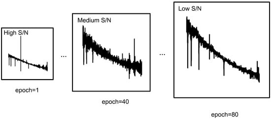
Figure 3.
Progressive learning of astronomical spectral data. Data with higher SNR are used at the beginning of training and data with lower SNR are used in the later stage.
4. Results
4.1. Dataset and Experimental Environment
Our experiments included two datasets. As outlined in Table 1, Dataset-A comprised 25,000 data entries, including A, F, G, M, and K stars. All spectra within this dataset exhibited S/N exceeding 5. Dataset-A was specifically employed for the stellar classification task. In contrast, dataset-B comprised 20,000 data entries dedicated exclusively to M stars, including subclasses 0–4. The S/N distribution for dataset-B is visualized in Figure 4, demonstrating that all spectra in this dataset possess S/N values less than 6. Dataset-B was utilized for the subclass classification of M stars. Across both datasets, 60% of the data were allocated for training, 20% for validation, and 20% for testing.

Table 1.
Description of dataset-A and dataset-B.
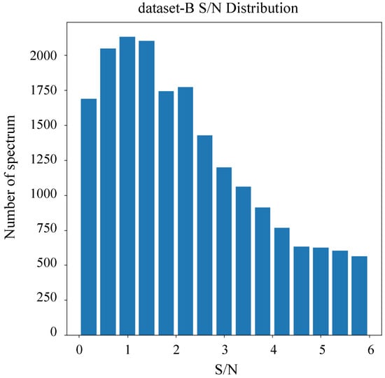
Figure 4.
The S/N distribution for dataset-B.
The classification performance of each model was evaluated using two primary metrics: accuracy and F1-score. Accuracy represents the ratio of correct predictions, including both true positives and true negatives, to the total number of predictions. Precision quantifies the proportion of true positive samples among all samples classified as positive, while recall represents the ratio of correctly classified positive samples to all true positive samples. The F1-score, a comprehensive performance metric, combines precision and recall. These metrics are mathematically defined as follows:
In the above equations, the terms are defined as follows: TP (true positive) refers to the count of positive samples predicted correctly, TN (true negative) signifies the count of negative samples predicted correctly, FP (false positive) represents the count of negative samples inaccurately predicted as positive, and FN (false negative) denotes the count of positive samples inaccurately predicted as negative. These metrics collectively provide a comprehensive assessment of the model’s classification performance.
All programs in this study were implemented in Python and executed on a desktop computer equipped with a 2.80 Ghz Intel(R) Core(TM) i9-10900F processor, 32 GB of RAM, a 64-bit Windows operating system, and an RTX 2080s GPU for computation.
4.2. Model Optimization
We embarked on a series of experiments designed to compare our model with other established techniques, including SVM [28], random forest [29], ANN [6], and 1D SSCNN [16]. Each experiment leveraged the two datasets outlined in Table 1. For all the models under evaluation (SVM, random forest, ANN, and 1D SSCNN) we engaged in diligent parameter tuning using both datasets. To achieve this, we conducted a comprehensive grid search across all parameters, utilizing the accuracy as the guiding metric to pinpoint the optimal parameter configurations. The experimental results of the models under various parameters can be found in Appendix A.
The model parameters of SVM include C and . In our study, we opted for the radial basis function (rbf) kernel function for SVM to achieve superior performance. The parameter ranges for each model were as follows:
- 1.
- C: 0.1, 1, 10, 100, 1000, 10,000
- 2.
- : 1, 0.1, 0.01, 0.001, 0.0001
For SVM, a total of 25 parameter combinations were considered. Each experiment involved five-fold cross-validation; the optimal model parameters for dataset-A were {‘C’: 10, ‘’: 0.01, ‘kernel’: ‘rbf’}, while the optimal parameters for dataset-B were {‘C’: 1000, ‘’: 0.0001, ‘kernel’: ‘rbf’}.
For the random forest model, the parameters included the number of trees in the forest, max_depth, min_samples_split, and min_samples_leaf. The parameter ranges were as follows:
- 1.
- max_depth: 20, 30, 40
- 2.
- min_samples_leaf: 1, 2, 5
- 3.
- min_samples_split: 2, 5, 10
- 4.
- n_estimators: 300, 400, 500
There were a total of 81 parameter combinations. Each experiment involved five-fold cross-validation; the optimal model parameters for dataset-A were {‘max_depth’: 30, ‘min_samples_leaf’: 2, ‘min_samples_split’: 2, ‘n_estimators’: 300}, while the optimal model parameters for dataset-B were {‘max_depth’: 20, ‘min_samples_leaf’: 1, ‘min_samples_split’: 2, ‘n_estimators’: 400}.
For ANN, the model parameters included the activation function, , hidden_layer_sizes, learning_rate, and solver. The parameter ranges were as follows:
- 1.
- activation function: relu, tanh, logistic
- 2.
- : 0.0001, 0.05
- 3.
- hidden_layer_sizes: (100,), (200,), (300,)
- 4.
- learning_rate: constant, adaptive
- 5.
- solver: adam, sgd
A total of 72 parameter combinations were considered. Each experiment was subjected to five-fold cross-validation; the optimal model parameters for dataset-A were {‘activation function’: ‘relu’, ‘’: 0.0001, ‘hidden_layer_sizes’: (100,), ‘learning_rate’: ‘adaptive’, ‘solver’: ‘adam’}, while the optimal model parameters for dataset-B were {‘activation function’: ‘relu’, ‘’: 0.0001, ‘hidden_layer_sizes’: (100,), ‘learning_rate’: ‘adaptive’, ‘solver’: ‘adam’}.
The model parameters of the 1D SSCNN included the learning rate and dropout rate; the range of each model parameter was as follows:
- 1.
- learning_rate: 0.01, 0.005, 0.001, 0.0005, 0.0001
- 2.
- dropout_rate: 0, 0.1, 0.3, 0.5
There were 20 parameter combinations in total. The optimal parameters for dataset-A were {learning_rate: 0.0005, dropout_rate: 0.3}, while the optimal parameters for dataset-B were {learning_rate: 0.0005, dropout_rate: 0.1}.
Finally, regarding our proposed model, the initial learning rate was set to 0.01, the cosine annealing algorithm [30] was employed to adjust it to 0.001 during training, the dropout rate was chosen as 0.2, and the stochastic gradient descent method [31] was utilized.
4.3. Experimental Results
Table 2 presents the experimental results for dataset-A, including the accuracy and F1-score for each class. Our model exhibits superior accuracy compared to the other tested models. Furthermore, we conducted a comparison within our model to examine the performance when using only image data or only spectral data. The results indicate that combining both images and spectra leads to improved experimental results. We additionally compared the results with and without data preprocessing, revealing that all metrics achieved with preprocessing outperform those without preprocessing. This underscores the importance of preprocessing in our experiment. However, in light of the high S/N of dataset-A and the relatively insignificant differences among all models, we place greater emphasis on the results for dataset-B.
Table 2.
Classification result for dataset-A. The text in bold indicates the highest performance according to the metrics (Training Time, Accuracy, and F1-Score).
For dataset-B, we specifically conducted subclass classification for M-class stars to further assess our model’s performance. Unlike dataset-A, the majority of training data in dataset-B feature low S/N, providing an opportunity to exhibit our model’s effectiveness in challenging conditions. We employed progressive training, as described in Section 3.5, to maximize the utilization of these data. The experimental results in Table 3 consistently demonstrate our model’s superior performance across all metrics. Notably, the model’s performance improves and the training time decreases with the application of progressive learning.
Table 3.
Classification results for dataset-B. The text in bold indicates the highest performance according to the metrics (Training Time, Accuracy, and F1-Score).
Finally, we replaced the attention mechanism in the EfficientNetV2 network structure with CBAM [25] to assess the effect of this modification. This comparison experiment was conducted on dataset-B, with only the attention mechanism being changed while keeping all other parameters constant. The results in Table 4 show that the experimental performance remains nearly unchanged when using ECA [24] instead of SE [23], while the training time is reduced. On the other hand, the experimental results with CBAM exhibit improvement along with a significant increase in training time, aligning with our earlier speculations in Section 3.2.
Table 4.
Classification with attention mechanism for dataset-B. The text in bold indicates the highest performance according to the metrics (Training Time, Accuracy, and F1-Score).
5. Discussion
Table 2 illustrates the excellent performance of all models on dataset-A, which is characterized by high S/N. Data with high S/N tend to yield good results even with simpler methods, making it challenging for models to exhibit substantial improvements. Consequently, our primary focus shifted to dataset-B, where most of the data have low S/N.
The random forest method performs well on dataset-A and poorly on dataset-B. This discrepancy may be attributed to random forest’s unsuitability for data with low S/N or subtle differences. However, because we did not specifically analyze the performance of the random forest model, we do not explore this matter further here. The random forest method was excluded from the subsequent analyses of model performance.
To emphasize our model’s advantages on low S/N data, we divided the test set of dataset-B into two subsets based on the S/N ratio. One subset contained data with an S/N ratio less than 2, while the other contained data with an S/N ratio greater than 2. We calculated the accuracy for each subset, as shown in Figure 5. Our model, especially when trained with the progressive training method, exhibits a significant advantage on the low S/N subset. In contrast, all models show minimal differences on the high S/N subset. These findings further validate our model’s superiority in handling low S/N data.
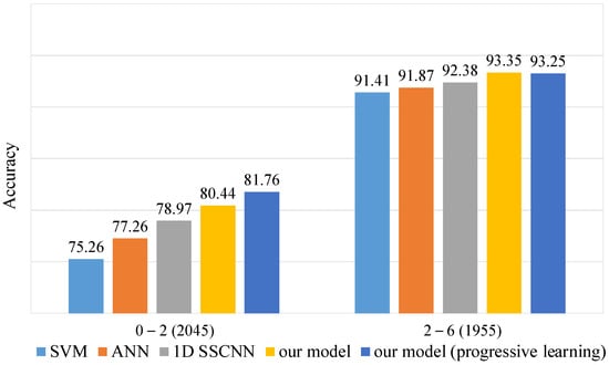
Figure 5.
Accuracy on dataset-B test set at different S/N levels. The test set of 4000 spectra was divided into 2045 spectra and 1955 spectra according to S/N levels of 0–2 and 2–6.
Additionally, we generated confusion matrices for each model using the test set of dataset-B, which are depicted in Figure 6 and Figure 7. Our model does not exhibit substantial improvements on M0 and M1, corresponding to relatively high average S/N ratios. However, it demonstrates significant enhancements on M2, M3, and M4, which represent low S/N scenarios.
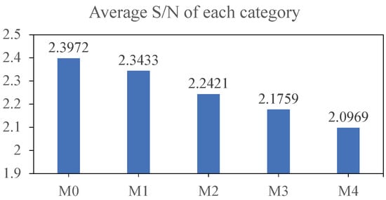
Figure 6.
Average S/N for each category of the dataset-B test set.
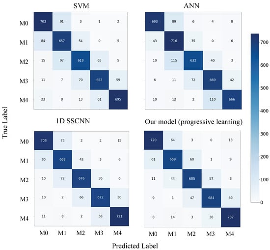
Figure 7.
Confusion matrix for each model on the dataset-B test set.
Furthermore, we analyzed the contribution of each component of our model by plotting confusion matrices for each component with and without the use of progressive learning, as shown in Figure 8. On M4, which has the lowest average S/N ratio, the model with both image and spectral components outperforms the models with only one of these components. This suggests that our model can effectively combine the strengths of both image and spectral data, resulting in improved overall accuracy. Additionally, our model with progressive learning exhibits enhanced accuracy in most categories, particularly M4, thanks to the progressive learning technique.
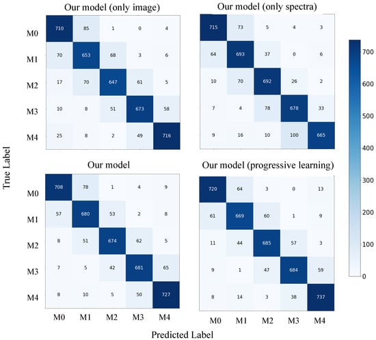
Figure 8.
Confusion matrix for our model on dataset-B test set.
In summary, the main contributions of this study are as follows:
1. We propose a novel approach to spectral classification using spectral images utilizing EfficientNetV2 and optimizing it for astronomical data, which yields promising results.
2. We design a model that effectively combines spectral images and 1D spectral data, which is particularly beneficial for low S/N data; this is particularly significant in light of the prevalence of the low S/N ratios prevalent in astronomical data.
6. Conclusions
In this study, we present a novel approach to spectral classification that departs from traditional methods. Our model integrates both spectral images and 1D spectral data, leveraging the features extracted from both for classification. For the image component, we employ EfficientNetV2 with specific optimizations for astronomical data. To process the raw spectral data, we introduce a new 1DCNN architecture.
We evaluated our model using spectra from SDSS DR16 and conducted experiments on two datasets: one for stellar spectral classification, and another for M-class stellar subclass classification. Our model achieved remarkable results, with an accuracy of 94.62% on the stellar spectral classification test set (dataset-A) and 87.38% on the M-class stellar subclass classification test set (dataset-B). These results outperformed the other tested models, particularly in the challenging scenario of M-class subclass classification with low S/N data.
Our model’s strength lies in its ability to handle data with lower S/N levels; this is a crucial aspect in astronomy, where a significant portion of the data exhibit low S/N levels.
Author Contributions
Conceptualization, W.W. and M.Q.; methodology, J.W.; software, J.W.; validation, J.W.; formal analysis, Y.Z. and W.W.; investigation, B.J.; resources, B.J.; writing—original draft preparation, J.W.; writing—review and editing, W.W.; visualization, B.J.; supervision, W.W.; project administration, W.W.; funding acquisition, Y.Z. All authors have read and agreed to the published version of the manuscript.
Funding
The study was funded by the National Natural Science Foundation of China under grant nos. 12273076 and 12133001, the China Manned Space Project under science research grant nos. CMS-CSST-2021-A04 and CMS-CSST-2021-A06, and the Natural Science Foundation of Hebei Province under grant no. A2018106014. Funding for the Sloan Digital Sky Survey IV has been provided by the Alfred P. Sloan Foundation, the U.S. Department of Energy Office of Science, and the participating institutions.
Data Availability Statement
The data underlying this article are available in SDSS at https://dr16.sdss.org/ (catalog data), accessed on 7 November 2023.
Acknowledgments
SDSS acknowledges support and resources from the Center for High-Performance Computing at the University of Utah. The SDSS web site is www.sdss.org. We acknowledge the use of spectra from SDSS.
Conflicts of Interest
The authors declare no conflict of interest. The funders had no role in the design of the study, in the collection, analysis, or interpretation of data, in the writing of the manuscript, or in the decision to publish the results.
Appendix A. Model Parameter Tuning Process
Appendix A.1. Optimal Model Parameter Selection of SVM for Dataset-A
The model parameters of SVM included C and . In this study, in order to obtain better performance, RBF (Radial Basis Function) was selected as the kenel function, and the range of each model parameter was as follows:
- 1.
- C: 0.1, 1, 10, 100, 1000, 10,000
- 2.
- : 1, 0.1, 0.01, 0.001, 0.0001
There were 25 parameter combinations in total. Each experiment was subject to five-fold cross-validation, and all results are listed in Table A1. As shown in Table A1, the optimal model parameters are {‘C’: 10, ‘’: 0.01, ‘kernel’: ‘rbf’}.
Table A1.
Model parameters and performance of SVM for dataset-A. The text in bold indicates the highest performance according to the Accuracy.
Table A1.
Model parameters and performance of SVM for dataset-A. The text in bold indicates the highest performance according to the Accuracy.
| C | Kernel | Accuracy (%) | B | Kernel | Accuracy (%) | ||
|---|---|---|---|---|---|---|---|
| 0.1 | 1 | rbf | 35.22 | 100 | 1 | rbf | 63.89 |
| 0.1 | 0.1 | rbf | 83.48 | 100 | 0.1 | rbf | 90.76 |
| 0.1 | 0.01 | rbf | 82.67 | 100 | 0.01 | rbf | 90.93 |
| 0.1 | 0.001 | rbf | 78.69 | 100 | 0.001 | rbf | 90.73 |
| 0.1 | 0.0001 | rbf | 73.40 | 100 | 0.0001 | rbf | 88.45 |
| 1 | 1 | rbf | 62.01 | 1000 | 1 | rbf | 63.89 |
| 1 | 0.1 | rbf | 89.15 | 1000 | 0.1 | rbf | 90.76 |
| 1 | 0.01 | rbf | 87.55 | 1000 | 0.01 | rbf | 90.72 |
| 1 | 0.001 | rbf | 84.71 | 1000 | 0.001 | rbf | 89.62 |
| 1 | 0.0001 | rbf | 79.43 | 1000 | 0.0001 | rbf | 90.05 |
| 10 | 1 | rbf | 63.89 | 10,000 | 1 | rbf | 63.89 |
| 10 | 0.1 | rbf | 90.71 | 10,000 | 0.1 | rbf | 90.76 |
| 10 | 0.01 | rbf | 91.08 | 10,000 | 0.01 | rbf | 90.72 |
| 10 | 0.001 | rbf | 88.23 | 10,000 | 0.001 | rbf | 88.63 |
| 10 | 0.0001 | rbf | 85.65 | 10,000 | 0.0001 | rbf | 88.26 |
Appendix A.2. Optimal Model Parameter Selection of SVM for Dataset-B
Similar to dataset-A, the range of model parameters for SVM was as follows:
- 1.
- C: 0.1, 1, 10, 100, 1000, 10,000
- 2.
- : 1, 0.1, 0.01, 0.001, 0.0001
The results are described in Table A2. From Table A2, the optimal parameters are {‘C’: 1000, ‘’: 0.0001, ‘kernel’: ‘rbf’}.
Table A2.
Model parameters and performance of SVM for dataset-B. The text in bold indicates the highest performance according to the Accuracy.
Table A2.
Model parameters and performance of SVM for dataset-B. The text in bold indicates the highest performance according to the Accuracy.
| C | Kernel | Accuracy (%) | B | Kernel | Accuracy (%) | ||
|---|---|---|---|---|---|---|---|
| 0.1 | 1 | rbf | 24.72 | 100 | 1 | rbf | 42.96 |
| 0.1 | 0.1 | rbf | 50.51 | 100 | 0.1 | rbf | 74.88 |
| 0.1 | 0.01 | rbf | 51.43 | 100 | 0.01 | rbf | 80.78 |
| 0.1 | 0.001 | rbf | 39.38 | 100 | 0.001 | rbf | 83.02 |
| 0.1 | 0.0001 | rbf | 27.37 | 100 | 0.0001 | rbf | 76.48 |
| 1 | 1 | rbf | 40.87 | 1000 | 1 | rbf | 42.96 |
| 1 | 0.1 | rbf | 71.58 | 1000 | 0.1 | rbf | 74.86 |
| 1 | 0.01 | rbf | 72.04 | 1000 | 0.01 | rbf | 80.33 |
| 1 | 0.001 | rbf | 59.93 | 1000 | 0.001 | rbf | 82.23 |
| 1 | 0.0001 | rbf | 38.93 | 1000 | 0.0001 | rbf | 83.44 |
| 10 | 1 | rbf | 42.96 | 10,000 | 1 | rbf | 42.96 |
| 10 | 0.1 | rbf | 74.85 | 10,000 | 0.1 | rbf | 74.86 |
| 10 | 0.01 | rbf | 80.26 | 10,000 | 0.01 | rbf | 80.34 |
| 10 | 0.001 | rbf | 75.65 | 10,000 | 0.001 | rbf | 81.26 |
| 10 | 0.0001 | rbf | 60.98 | 10,000 | 0.0001 | rbf | 81.74 |
Appendix A.3. Optimal Model Parameter Selection of Random Forest for Dataset-A
For random forest, the model parameters included the number of trees in the forest, max_depth, min_samples split, and min_samp. In this study, the ranges for each model parameter were as follows:
- 1.
- max_depth: 20, 30, 40
- 2.
- min_samples_leaf: 1, 2, 5
- 3.
- min_samples_split: 2, 5, 10
- 4.
- n_estimators: 300, 400, 500
There were 81 parameter combinations in total. Each experiment used five-fold cross-validation, and part of the results are indicated in Table A3. As shown in Table A3, the optimal model parameters are {‘max_depth’: 30, ‘min_samples_leaf’: 2, ‘min_samples_split’: 2, ‘n_estimators’: 300}.
Table A3.
Model parameters and performance of random forest for dataset-A. The text in bold indicates the highest performance according to the Accuracy.
Table A3.
Model parameters and performance of random forest for dataset-A. The text in bold indicates the highest performance according to the Accuracy.
| Max_Depth | Min_Samples_Leaf | Min_Samples_Split | n_Estimators | Accuracy (%) |
|---|---|---|---|---|
| 20 | 1 | 2 | 300 | 88.71 |
| 20 | 1 | 2 | 400 | 88.62 |
| … | … | … | … | … |
| 30 | 1 | 10 | 400 | 88.78 |
| 30 | 1 | 10 | 500 | 88.67 |
| 30 | 2 | 2 | 300 | 88.86 |
| 30 | 2 | 2 | 400 | 88.64 |
| 30 | 2 | 2 | 500 | 88.59 |
| 30 | 2 | 5 | 300 | 88.61 |
| 30 | 2 | 5 | 400 | 88.59 |
| 30 | 2 | 5 | 500 | 88.83 |
| 30 | 2 | 10 | 300 | 88.59 |
| 30 | 2 | 10 | 400 | 88.51 |
| … | … | … | … | … |
| 40 | 1 | 2 | 300 | 88.70 |
| 40 | 1 | 2 | 400 | 88.79 |
| 40 | 1 | 2 | 500 | 88.79 |
| 40 | 5 | 10 | 300 | 88.47 |
| 40 | 5 | 10 | 400 | 88.59 |
| 40 | 5 | 10 | 500 | 88.51 |
Appendix A.4. Optimal Model Parameter Selection of Random Forest for Dataset-B
Similar to dataset-A, the range of each model parameter for random forest was as follows:
- 1.
- max_depth: 5, 10, 15, 20
- 2.
- min_samples_leaf: 1, 2, 5, 10
- 3.
- min_samples_split: 2, 10, 15, 100
- 4.
- n_estimators: 100, 200, 300, 400, 500
There were 320 parameter combinations in total. Each experiment was subject to five-fold cross-validation, and part of the results are shown in Table A4. From the table, the optimal model parameters are {‘max_depth’: 20, ‘min_samples_leaf’: 1, ‘min_samples_split’: 2, ‘n_estimators’: 400}.
Table A4.
Model parameters and performance of random forest for dataset-B. The text in bold indicates the highest performance according to the Accuracy.
Table A4.
Model parameters and performance of random forest for dataset-B. The text in bold indicates the highest performance according to the Accuracy.
| Max_Depth | Min_Samples_Leaf | Min_Samples_Split | n_Estimators | Accuracy (%) |
|---|---|---|---|---|
| 5 | 1 | 2 | 100 | 47.84 |
| 5 | 1 | 2 | 200 | 48.13 |
| … | … | … | … | … |
| 20 | 1 | 2 | 100 | 62.98 |
| 20 | 1 | 2 | 200 | 63.83 |
| 20 | 1 | 2 | 300 | 64.86 |
| 20 | 1 | 2 | 400 | 65.06 |
| … | … | … | … | … |
| 20 | 10 | 15 | 500 | 63.74 |
| 20 | 10 | 100 | 100 | 59.16 |
| 20 | 10 | 100 | 200 | 59.64 |
| 20 | 10 | 100 | 300 | 59.52 |
| 20 | 10 | 100 | 400 | 59.63 |
| 20 | 10 | 100 | 500 | 59.73 |
Appendix A.5. Optimal Model Parameter Selection of ANN for Dataset-A
The model parameters of ANN included activation function, , hidden_layer_sizes, learning_rate, and solver. In this study, the range of each model parameter was as follows:
- 1.
- activation function: relu, tanh, logistic
- 2.
- : 0.0001, 0.05
- 3.
- hidden_layer_sizes: (100,), (200,), (300,)
- 4.
- learning_rate: constant, adaptive
- 5.
- solver: adam, sgd
There were 72 parameter combinations in total. Each experiment was subject to five-fold cross-validation, and part of the results are shown in Table A5. As shown in Table A5, the optimal model parameters are {‘activation function’: ‘relu’, ‘’: 0.0001, ‘hidden_layer_sizes’: (100,), ‘learning_rate’: ‘adaptive’, ‘solver’: ‘adam’}.
Table A5.
Model parameters and performance of ANN for dataset-A. The text in bold indicates the highest performance according to the Accuracy.
Table A5.
Model parameters and performance of ANN for dataset-A. The text in bold indicates the highest performance according to the Accuracy.
| Activation Function | Hidden_Layer_Sizes | Learning_Rate | Solver | Accuracy (%) | |
|---|---|---|---|---|---|
| relu | 0.0001 | (100,) | constant | adam | 91.39 |
| relu | 0.0001 | (100,) | constant | sgd | 91.73 |
| relu | 0.0001 | (100,) | adaptive | adam | 92.76 |
| … | … | … | … | … | … |
| relu | 0.05 | (300,) | adaptive | adam | 90.80 |
| relu | 0.05 | (300,) | adaptive | sgd | 92.11 |
| tanh | 0.0001 | (100,) | constant | adam | 92.05 |
| tanh | 0.0001 | (100,) | constant | sgd | 91.03 |
| tanh | 0.0001 | (100,) | adaptive | adam | 91.83 |
| tanh | 0.0001 | (100,) | adaptive | sgd | 90.76 |
| tanh | 0.0001 | (200,) | constant | adam | 92.25 |
| tanh | 0.0001 | (200,) | constant | sgd | 90.49 |
| … | … | … | … | … | … |
| logistic | 0.05 | (200,) | adaptive | sgd | 84.46 |
| logistic | 0.05 | (300,) | constant | adam | 88.73 |
| logistic | 0.05 | (300,) | constant | sgd | 84.72 |
| logistic | 0.05 | (300,) | adaptive | adam | 89.56 |
| logistic | 0.05 | (300,) | adaptive | sgd | 84.82 |
Appendix A.6. Optimal Model Parameter Selection of ANN for Dataset-B
Similar to dataset-A, the range of model parameters for ANN was as follows:
- 1.
- activation function: relu, tanh, logistic
- 2.
- : 0.0001, 0.05
- 3.
- hidden_layer_sizes: (100,), (200,), (300,)
- 4.
- learning_rate: constant, adaptive
- 5.
- solver: adam, sgd
There were 72 parameter combinations in total. Each experiment used 5five-fold cross-validation, and part of the results are shown in Table A6. As indicated in Table A6, the optimal model parameters are {‘activation function’: ‘relu’, ‘’: 0.0001, ‘hidden_layer_sizes’: (100,), ‘learning_rate’: ‘adaptive’, ‘solver’: ‘adam’}.
Table A6.
Model parameters and performance of ANN for dataset-B. The text in bold indicates the highest performance according to the Accuracy.
Table A6.
Model parameters and performance of ANN for dataset-B. The text in bold indicates the highest performance according to the Accuracy.
| Activation Function | Hidden_Layer_Sizes | Learning_Rate | Solver | Accuracy (%) | |
|---|---|---|---|---|---|
| relu | 0.0001 | (100,) | constant | adam | 81.48 |
| relu | 0.0001 | (100,) | constant | sgd | 80.95 |
| relu | 0.0001 | (100,) | adaptive | adam | 82.90 |
| relu | 0.05 | (200,) | adaptive | sgd | 80.95 |
| relu | 0.05 | (300,) | constant | adam | 79.24 |
| relu | 0.05 | (300,) | constant | sgd | 80.78 |
| relu | 0.05 | (300,) | adaptive | adam | 82.07 |
| relu | 0.05 | (300,) | adaptive | sgd | 81.43 |
| … | … | … | … | … | …. |
| tanh | 0.0001 | (100,) | constant | sgd | 80.29 |
| tanh | 0.0001 | (100,) | adaptive | adam | 80.75 |
| tanh | 0.05 | (300,) | constant | sgd | 81.08 |
| tanh | 0.05 | (300,) | adaptive | adam | 81.15 |
| … | … | … | … | … | … |
| logistic | 0.05 | (300,) | constant | adam | 78.41 |
| logistic | 0.05 | (300,) | constant | sgd | 73.76 |
| logistic | 0.05 | (300,) | adaptive | adam | 75.55 |
| logistic | 0.05 | (300,) | adaptive | sgd | 73.60 |
Appendix A.7. Optimal Model Parameter Selection of 1D SSCNN for Dataset-A
The model parameters of 1D SSCNN included the learning rate and dropout rate. The range of each model parameter was as follows:
- 1.
- learning_rate: 0.01, 0.005, 0.001, 0.0005, 0.0001
- 2.
- dropout_rate: 0, 0.1, 0.3, 0.5
There were 20 parameter combinations in total. The results are shown in Table A7. From the table, the optimal parameters are {learning_rate: 0.0005, dropout_rate: 0.3}.
Table A7.
Model parameters and performance of 1D SSCNN for dataset-A. The text in bold indicates the highest performance according to the Accuracy.
Table A7.
Model parameters and performance of 1D SSCNN for dataset-A. The text in bold indicates the highest performance according to the Accuracy.
| Learning_Rate | Dropout_Rate | Accuracy (%) | Learning_Rate | Dropout_Rate | Accuracy (%) |
|---|---|---|---|---|---|
| 0.01 | 0 | 20.00 | 0.01 | 0.3 | 20.00 |
| 0.005 | 0 | 42.38 | 0.005 | 0.3 | 89.42 |
| 0.001 | 0 | 85.53 | 0.001 | 0.3 | 92.52 |
| 0.0005 | 0 | 84.97 | 0.0005 | 0.3 | 93.04 |
| 0.0001 | 0 | 85.05 | 0.0001 | 0.3 | 92.26 |
| 0.01 | 0.1 | 20.00 | 0.01 | 0.5 | 20.00 |
| 0.005 | 0.1 | 89.38 | 0.005 | 0.5 | 88.30 |
| 0.001 | 0.1 | 92.46 | 0.001 | 0.5 | 92.38 |
| 0.0005 | 0.1 | 92.88 | 0.0005 | 0.5 | 92.54 |
| 0.0001 | 0.1 | 91.96 | 0.0001 | 0.5 | 91.76 |
Appendix A.8. Optimal Model Parameter Selection of 1D SSCNN for Dataset-B
Similar to dataset-A, the range of model parameters for 1D SSCNN was as follows:
- 1.
- learning_rate: 0.01, 0.005, 0.001, 0.0005, 0.0001
- 2.
- dropout_rate: 0, 0.1, 0.3, 0.5
The results are shown in Table A8. From the table, the optimal parameters are {learning_rate: 0.0005, dropout_rate: 0.1}.
Table A8.
Model parameters and performance of 1D SSCNN for dataset-B. The text in bold indicates the highest performance according to the Accuracy.
Table A8.
Model parameters and performance of 1D SSCNN for dataset-B. The text in bold indicates the highest performance according to the Accuracy.
| Learning_Rate | Dropout_Rate | Accuracy (%) | Learning_Rate | Dropout_Rate | Accuracy (%) |
|---|---|---|---|---|---|
| 0.01 | 0 | 20.00 | 0.01 | 0.3 | 20.00 |
| 0.005 | 0 | 42.38 | 0.005 | 0.3 | 57.88 |
| 0.001 | 0 | 85.53 | 0.001 | 0.3 | 84.45 |
| 0.0005 | 0 | 84.97 | 0.0005 | 0.3 | 85.60 |
| 0.0001 | 0 | 85.05 | 0.0001 | 0.3 | 85.70 |
| 0.01 | 0.1 | 20.00 | 0.01 | 0.5 | 20.00 |
| 0.005 | 0.1 | 29.38 | 0.005 | 0.5 | 53.08 |
| 0.001 | 0.1 | 85.28 | 0.001 | 0.5 | 84.68 |
| 0.0005 | 0.1 | 86.13 | 0.0005 | 0.5 | 85.63 |
| 0.0001 | 0.1 | 85.20 | 0.0001 | 0.5 | 85.90 |
Notes
| 1 | https://skyserver.sdss.org/CasJobs/, accessed on 7 November 2023. |
| 2 | https://matplotlib.org/stable/, accessed on 7 November 2023. |
References
- York, D.G.; Adelman, J.; John, E.; Anderson, J.; Anderson, S.F.; Annis, J.; Bahcall, N.A.; Bakken, J.A.; Barkhouser, R.; Bastian, S.; et al. The Sloan Digital Sky Survey: Technical Summary. Astron. J. 2000, 120, 1579–1587. [Google Scholar] [CrossRef]
- Cui, X.Q.; Zhao, Y.H.; Chu, Y.Q.; Li, G.P.; Li, Q.; Zhang, L.P.; Su, H.J.; Yao, Z.Q.; Wang, Y.N.; Xing, X.Z.; et al. The Large Sky Area Multi-Object Fiber Spectroscopic Telescope (LAMOST). Res. Astron. Astrophys. 2012, 12, 1197–1242. [Google Scholar] [CrossRef]
- Morgan, W.W.; Keenan, P.C. Spectral Classification. Annu. Rev. Astron. Astrophys. 1973, 11, 29–50. [Google Scholar] [CrossRef]
- Duan, F.Q.; Liu, R.; Guo, P.; Zhou, M.Q.; Wu, F.C. Automated spectral classification using template matching. Res. Astron. Astrophys. 2009, 9, 341. [Google Scholar] [CrossRef]
- Bolton, A.S.; Schlegel, D.J.; Éric, A.; Bailey, S.; Bhardwaj, V.; Brownstein, J.R.; Burles, S.; Chen, Y.M.; Dawson, K.; Eisenstein, D.J.; et al. Spectral classification and redshift measurement for the sdss-III baryon oscillation spectroscopic survey. Astron. J. 2012, 144, 144. [Google Scholar] [CrossRef]
- von Hippel, T.; Storrie-Lombardi, L.J.; Storrie-Lombardi, M.C.; Irwin, M.J. Automated classification of stellar spectra—I. Initial results with artificial neural networks. Mon. Not. R. Astron. Soc. 1994, 269, 97–104. [Google Scholar] [CrossRef]
- Singh, H.P.; Gulati, R.K.; Gupta, R. Stellar Spectral Classification using Principal Component Analysis and Artificial Neural Networks. Mon. Not. R. Astron. Soc. 1998, 295, 312–318. [Google Scholar] [CrossRef]
- Navarro, S.G.; Corradi, R.L.M.; Mampaso, A. Automatic spectral classification of stellar spectra with low signal-to-noise ratio using artificial neural networks. Astron. Astrophys. 2012, 538, A76. [Google Scholar] [CrossRef]
- Gray, R.O.; Corbally, C.J. An Expert Computer Program for Classifying Stars on the MK Spectral Classification System. Astron. J. 2014, 147, 80. [Google Scholar] [CrossRef]
- Li, X.R.; Lin, Y.T.; Qiu, K.B. Stellar spectral classification and feature evaluation based on a random forest. Res. Astron. Astrophys. 2019, 19, 111. [Google Scholar] [CrossRef]
- Kheirdastan, S.; Bazarghan, M. SDSS-DR12 bulk stellar spectral classification: Artificial neural networks approach. Astrophys. Space Sci. 2016, 361, 304. [Google Scholar] [CrossRef][Green Version]
- Liu, Z.b.; Zhao, W.J. An unbalanced spectra classification method based on entropy. Astrophys. Space Sci. 2017, 362, 98. [Google Scholar] [CrossRef]
- Yang, H.; Zhou, L.; Cai, J.; Shi, C.; Yang, Y.; Zhao, X.; Duan, J.; Yin, X. Data mining techniques on astronomical spectra data – II. Classification analysis. Mon. Not. R. Astron. Soc. 2022, 518, 5904–5928. [Google Scholar] [CrossRef]
- Fabbro, S.; Venn, K.A.; O’Briain, T.; Bialek, S.; Kielty, C.L.; Jahandar, F.; Monty, S. An application of deep learning in the analysis of stellar spectra. Mon. Not. R. Astron. Soc. 2018, 475, 2978–2993. [Google Scholar] [CrossRef]
- Sharma, K.; Kembhavi, A.; Kembhavi, A.; Sivarani, T.; Abraham, S.; Vaghmare, K. Application of convolutional neural networks for stellar spectral classification. Mon. Not. R. Astron. Soc. 2020, 491, 2280–2300. [Google Scholar] [CrossRef]
- Liu, W.; Zhu, M.; Dai, C.; He, D.Y.; Yao, J.; Tian, H.F.; Wang, B.Y.; Wu, K.; Zhan, Y.; Chen, B.Q.; et al. Classification of large-scale stellar spectra based on deep convolutional neural network. Mon. Not. R. Astron. Soc. 2019, 483, 4774–4783. [Google Scholar] [CrossRef]
- Zou, Z.; Zhu, T.; Xu, L.; Luo, A.L. Celestial Spectra Classification Network Based on Residual and Attention Mechanisms. Publ. Astron. Soc. Pac. 2020, 132, 044503. [Google Scholar] [CrossRef]
- Sandler, M.; Howard, A.; Zhu, M.; Zhmoginov, A.; Chen, L.C. MobileNetV2: Inverted Residuals and Linear Bottlenecks. In Proceedings of the 2018 IEEE/CVF Conference on Computer Vision and Pattern Recognition, Salt Lake City, UT, USA, 18–23 June 2018; pp. 4510–4520. [Google Scholar] [CrossRef]
- Yuan, L.; Chen, Y.; Wang, T.; Yu, W.; Shi, Y.; Jiang, Z.; Tay, F.E.H.; Feng, J.; Yan, S. Tokens-to-Token ViT: Training Vision Transformers from Scratch on ImageNet. In Proceedings of the 2021 IEEE/CVF International Conference on Computer Vision (ICCV), Montreal, BC, Canada, 11–17 October 2021; pp. 538–547. [Google Scholar] [CrossRef]
- Tan, M.; Le, Q. EfficientNetV2: Smaller Models and Faster Training. In Proceedings of the 38th International Conference on Machine Learning, Online, 18–24 July 2021; Meila, M., Zhang, T., Eds.; PMLR, Proceedings of Machine Learning Research: San Diego, CA, USA, 2021; Volume 139, pp. 10096–10106. [Google Scholar] [CrossRef]
- Mahdi, B. Automated classification of ELODIE stellar spectral library using probabilistic artificial neural networks. Bull. Astron. Soc. India 2008, 36, 1–54. [Google Scholar] [CrossRef]
- Tan, M.; Le, Q. Efficientnet: Rethinking model scaling for convolutional neural networks. arXiv 2019, arXiv:1905.11946. [Google Scholar]
- Jie, H.; Li, S.; Gang, S.; Albanie, S. Squeeze-and-Excitation Networks. In Proceedings of the 2018 IEEE/CVF Conference on Computer Vision and Pattern Recognition, Salt Lake City, UT, USA, 18–23 June 2018. [Google Scholar] [CrossRef]
- Wang, Q.; Wu, B.; Zhu, P.; Li, P.; Hu, Q. ECA-Net: Efficient Channel Attention for Deep Convolutional Neural Networks. In Proceedings of the 2020 IEEE/CVF Conference on Computer Vision and Pattern Recognition (CVPR), Seattle, WA, USA, 13–19 June 2020. [Google Scholar] [CrossRef]
- Woo, S.; Park, J.; Lee, J.Y.; Kweon, I.S. CBAM: Convolutional Block Attention Module; Springer: Cham, Switzerland, 2018. [Google Scholar] [CrossRef]
- Ioffe, S.; Szegedy, C. Batch normalization: Accelerating deep network training by reducing internal covariate shift. arXiv 2015, arXiv:1502.03167. [Google Scholar]
- Lin, T.Y.; Goyal, P.; Girshick, R.; He, K.; Dollár, P. Focal Loss for Dense Object Detection. arXiv 2017, arXiv:1708.02002. [Google Scholar]
- Hearst, M.; Dumais, S.; Osuna, E.; Platt, J.; Scholkopf, B. Support vector machines. IEEE Intell. Syst. Their Appl. 1998, 13, 18–28. [Google Scholar] [CrossRef]
- Breiman, L. Random Forests. Mach. Learn. 2001, 45, 5–32. [Google Scholar] [CrossRef]
- Loshchilov, I.; Hutter, F. SGDR: Stochastic Gradient Descent with Warm Restarts. arXiv 2016, arXiv:1608.03983. [Google Scholar]
- Jin, J.; Fu, K.; Zhang, C. Traffic Sign Recognition with Hinge Loss Trained Convolutional Neural Networks. IEEE Trans. Intell. Transp. Syst. 2014, 15, 1991–2000. [Google Scholar] [CrossRef]


Disclaimer/Publisher’s Note: The statements, opinions and data contained in all publications are solely those of the individual author(s) and contributor(s) and not of MDPI and/or the editor(s). MDPI and/or the editor(s) disclaim responsibility for any injury to people or property resulting from any ideas, methods, instructions or products referred to in the content. |
© 2023 by the authors. Licensee MDPI, Basel, Switzerland. This article is an open access article distributed under the terms and conditions of the Creative Commons Attribution (CC BY) license (https://creativecommons.org/licenses/by/4.0/).