Abstract
The standard formulation of General Relativity Theory, in the absence of a cosmological constant, is unable to explain the responsible mechanism for the observed late-time cosmic acceleration. On the other hand, by inserting the cosmological constant in Einstein’s field equations, it is possible to describe the cosmic acceleration, but the cosmological constant suffers from an unprecedented fine-tuning problem. This motivates one to modify Einstein’s spacetime geometry of General Relativity. The modified theory of gravity is an alternative theory to General Relativity, where the non-metricity scalar Q is the responsible candidate for gravitational interactions. In the present work, we consider a Friedmann–Lemâitre–Robertson–Walker cosmological model dominated by bulk viscous cosmic fluid in gravity with the functional form , where and n are free parameters of the model. We constrain our model with the Pantheon supernovae dataset of 1048 data points, the Hubble dataset of 31 data points, and the baryon acoustic oscillations dataset consisting of 6 data points. We find that our cosmological model efficiently describes the observational data. We present the evolution of our deceleration parameter with redshift, and it properly predicts a transition from decelerated to accelerated phases of the universe’s expansion. Furthermore, we present the evolution of density, bulk viscous pressure, and the effective equation of state parameter with redshift. Those show that bulk viscosity in a cosmic fluid is a valid candidate to acquire the negative pressure to drive the cosmic expansion efficiently. We also examine the behavior of different energy conditions to test the viability of our cosmological model. Furthermore, the statefinder diagnostics are also investigated in order to distinguish among different dark energy models.
1. Introduction
The acceleration of the universe’s expansion is one of the most active discoveries of modern cosmology. Observational studies include Type Ia supernovae [1,2], large-scale structure [3,4], baryon acoustic oscillations [5,6], and cosmic microwave background radiation [7,8]. The reason behind the late-time acceleration is a mystery. Several models hypothesize the existence of a component called dark energy, which makes up around 70% of the entire universe and could possess the feature of speeding up the universe’s expansion.
The cosmological constant in the General Relativity (GR) field equations plays the role of dark energy, i.e., a fluid with constant energy density and high negative pressure. There are some issues with the cosmological constant model, such as the cosmic coincidence problem [9], which is the fact that the density of non-relativistic matter and dark energy is the same order today. A more delicate issue surrounding the cosmological constant is the so-called cosmological constant problem, which is the high discrepancy between the astronomically observed value of [1,2] and the particle physics theoretically predicted value of the quantum vacuum energy [10].
With the main purpose of solving the above cosmological issues, dynamical (time-varying) dark energy models such as the Chaplygin gas model [11,12], k-essence [13,14], quintessence [15,16], and decaying vacuum models [17,18,19,20] have been proposed for some time in the literature.
Modified theories of gravity have also been intensively investigated to understand the origin of the cosmic acceleration, as well as to address the cosmological constant model problems. It is possible to predict late-time cosmic acceleration by modifying GR action. Some possibilities can be seen within the [21,22,23], [24,25], [26], and [27,28,29,30] theories of gravitation, with R, G, , and T being, respectively, the Ricci, Gauss–Bonnet, energy–momentum, and torsion scalars.
In the present article, we will work with the recently introduced theory of gravity [31], for which Q is the non-metricity scalar, to be presented below. The gravity is an extension of GR that describes the spacetime geometry by the non-vanishing curvature in the absence of torsion and non-metricity, whereas the gravity generalizes the teleparallel equivalent of GR (TEGR), in which the gravitational interactions are attributed to the non-zero torsion with vanishing curvature and non-metricity. Finally, the theory of gravity, which will be described in Section 2, is an extension of the symmetric teleparallel equivalent of GR (STEGR), where the complete charge of gravitational interactions attributed to the non-metricity term with zero curvature and torsion. The non-metricity formulation was discussed earlier by Hehl and Ne’eman (see References [32,33,34,35]). The symmetric teleparallel gravity is proven in the so-called coincidence gauge by imposing that the connection is symmetric [36]. The Weyl geometry is also observed to be a particular example of the Weyl–Cartan geometry, in which torsion disappears. The non-metricity is interpreted as a massless spin three-field in the case of symmetric connections [37,38]. Furthermore, it is noted in the literature that, due to the appearance of non-metricity, the light cone structure is not preserved during parallel transport [39]. Further, fermions are an issue in TEGR because they couple to the axial contorsion of the Weitzenbock connection. This difficulty is eliminated in STEGR since Dirac fermions only couple to the completely antisymmetric component of the affine connection and are unaffected by any disformation piece.
Although recently proposed, the gravity theory already presents some interesting and valuable applications in the literature [40,41,42,43,44,45,46,47,48,49]. The first cosmological solutions in the gravity appear in References [50,51], while the cosmography and energy conditions can, respectively, be seen in [52,53].
Here, we are going to consider the cosmology in the presence of a viscous fluid. When a cosmic fluid expands too fast, the recovering of thermodynamic equilibrium generates an effective pressure. The high viscosity in a cosmic fluid is the manifestation of such an effective pressure [54,55].
Basically, there are two viscosity coefficients, namely shear viscosity and bulk viscosity. Shear viscosity is related to velocity gradients in the fluid, and by considering the universe as described by the homogeneous and isotropic Friedmann–Lemâitre–Robertson–Walker (FLRW) background, it can be omitted. Anyhow, by dropping the assumption of the homogeneity and isotropy of the universe, several cosmological models with shear viscosity fluid have been constructed, as one can check, for instance, in [56,57,58,59]. On the other hand, bulk viscosity, which we are going to consider here, introduces damping associated with volumetric straining. To become familiar with bulk viscous fluid cosmological models, one can check References [60,61,62,63,64,65,66,67]. Moreover, some interesting applications of bulk viscous cosmology in black holes are presented in [68,69].
Researchers examine dark energy reconstruction with numerous observations as the data increase. The majority of studies have been concentrated on observable evidence from Type Ia supernovae, cosmic microwave background, and baryon acoustic oscillations (BAOs), which are known to be helpful in constraining cosmological models. The Hubble parameter dataset shows the intricate structure of the expansion of the universe. The ages of the most massive and slowly evolving galaxies offer direct measurements of the Hubble parameter at various redshifts z, resulting in the development of a new form of standard cosmological probe [70].
In our present work, we include 31 measurements of Hubble expansion spanned using the differential age method [71] and BAO data consisting of six points [72]. Scolnic et al. published a large Type Ia supernovae sample named Pantheon, with 1048 points and covering the redshift range [73]. Our analysis uses the , BAO, and Pantheon samples to constrain the cosmological model.
This work aims to describe the recently observed late-time acceleration with the help of the bulk viscosity of the cosmic fluid (without including any dark energy component) in the framework of the theory of gravity. The manuscript is organized as follows: in Section 2, we discuss the gravity formalism. In Section 3, we describe the FLRW universe dominated by bulk viscous non-relativistic matter and derive the expression for the Hubble parameter and the deceleration parameter. Further, in Section 4, we analyze the observational data to find the best-fit ranges for the parameters using the Hubble dataset containing 31 points, the BAO sample, and the Pantheon dataset of 1048 samples. Moreover, we analyze the behavior of different cosmological parameters such as Hubble, density, effective pressure, deceleration parameter, and effective equation of state (EoS) parameter. In Section 5, we investigate the consistency of our bulk viscous fluid model by analyzing the different energy conditions. In Section 6, we analyze the behavior of statefinder parameters on the values constrained by the observational data to differentiate between dark energy models. Lastly, we discuss our results in Section 7.
2. Fundamental Formulations in Gravity
In gravity theory, the spacetime is established with the help of the non-metricity and symmetric teleparallelism condition, i.e., and in an torsionless environment. Hence, the associated affine connection is given by
with
being the Christoffel symbols and the distortion tensor, respectively, where
is the non-metricity tensor.
In addition, the superpotential tensor or non-metricity conjugate is given by
Then, the trace of the non-metricity tensor can be acquired as [74]
The definition of the energy–momentum tensor for matter is
Furthermore, one can obtain the following relation between the curvature tensor and corresponding to the connection and as
and so,
Here, is an invertible relation. Hence, it is always possible to find a coordinate system so that the connection vanishes. This situation is called the coincident gauge, and the covariant derivative reduces to the partial one . However, in any other coordinate system in which this affine connection does not vanish, the metric evolution will be affected and result in a completely different theory [75,76]. Thus, in the coincident gauge coordinate, we have
while, in an arbitrary coordinate system,
Locally, GR does not distinguish between gravitational and inertial effects; however, by invoking frame fields, it is possible to covariantly define gravitational energy in the teleparallel approach [77]. The canonical frame is identified in the absence of both curvature and torsion and the canonical coordinates in the absence of inertial effects. New physics can emerge from such a formalism. Symmetric teleparallel gravity is broadly derived in three gravity theories based on the coordinate transformations [78]. In this case, we use the spatially flat case, i.e., the gravity, whose field equations are much easier to understand.
The gravity is described by the action [31]:
in which is an arbitrary function of the non-metricity, , and is the Lagrangian density of matter. One can check in Reference [31] that the functional form corresponds to the symmetric teleparallel equivalent to General Relativity (STEGR) limit.
The gravitational field equations obtained by varying the action (16) with respect to the metric are
in which we define .
3. The Cosmological Model
We consider the flat FLRW metric for our analysis [79], such that:
In Equation (18) above, is the cosmic scale factor, as usual.
From now on, we will fix the coincident gauge so that connection becomes trivial and the metric is only a fundamental variable.
We are going to assume a bulk viscous fluid, and below, we present some considerations favoring such an assumption.
Firstly, considering bulk viscosity in a fluid can be seen as an attempt to refine its description, minimizing its ideal properties. This can be checked, for instance, in the stellar astrophysics realistic models in References [80,81,82].
Under the conditions of spatial homogeneity and isotropy (which refers to the cosmological principle, as one can check, for instance, in Reference [83]), the bulk viscous pressure is the unique admissible dissipative phenomenon. In a gas dynamical model, the existence of an effective bulk pressure can be traced back to a non-standard self-interacting force on the particles of the gas [63]. The bulk viscosity contributes negatively to the total pressure, as one can check, for instance, in References [84,85,86].
Due to spatial isotropy, the bulk viscous pressure is the same in all spatial directions and, hence, proportional to the volume expansion , with being the Hubble parameter and the dot representing the time derivative.
The effective pressure of the cosmic fluid becomes [87,88,89]
in which p is the usual pressure and is the bulk viscosity coefficient, which we will assume as a free parameter of the model.
The corresponding energy–momentum tensor is given by
in which is the matter–energy density and the four-velocity is such that its components are .
The relation between normal pressure and matter–energy density follows [90] , with being a constant lying in the range . Then, the effective equation of state for the bulk viscous fluid is given by the following:
The Friedmann-like equations for our gravitational model are obtained from the substitution of Equations (18)–(21) into Equation (11) and read as follows (check, for instance, References [74,91]):
In particular, for , we retrieve the usual Friedmann equations [91], as expected, since, as we have mentioned above, this particular choice for the functional form of the function is the STEGR limit of the theory.
For our investigation of the bulk viscosity fluid cosmological model, we consider the following functional form:
with and constant n. This particular functional form for was motivated by a polynomial form applied, for instance, in Reference [53]. Note that the parameter n considered in our model is not the spectral index; rather, it is a free model parameter.
For the above choice of the function (Equation (24)), we rewrite Equations (22)–(23) as follows
in which, for the former, we isolated .
Now, we replace the term by via the expression , such that Equation (27) becomes
The integration of Equation (28) yields the following solution:
with being a constant of integration to be found below.
4. Observational Constraints
To examine the observational features of our cosmological model, we used the cosmic Hubble and supernovae observations. We used the 31 points of the Hubble datasets, the 6 points of the BAO datasets, and the 1048 points from the Pantheon supernovae samples. We applied the Bayesian analysis and likelihood function along with the Markov chain Monte Carlo (MCMC) method in the emcee python library [92].
4.1. Hubble Datasets
The Hubble parameter can be expressed as . As is derived from a spectroscopic survey, the model-independent value of the Hubble parameter may be calculated by measuring the quantity .
We incorporated the set of 31 data points that are measured from the differential age approach [93] to avoid extra correlation with the BAO data. The mean values of the model parameters , , and n are calculated using the chi-squared function as follows:
Here, is the Hubble parameter value predicted by the model, represents its observed value, and the standard error in the observed value of H is .
Figure 1 shows the error bar plot of the considered model and the CDM or standard cosmological model, with cosmological constant density parameter , matter density parameter , and km/s/Mpc.
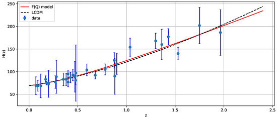
Figure 1.
The error bar plot of H versus z for the considered model. The solid red line is the curve for the model, whereas the black dotted line represents the CDM model. The blue dots depict the 31 points of the Hubble data.
4.2. BAO Datasets
The BAO distance dataset, which includes the 6dFGS, SDSS, and WiggleZ surveys, comprises BAO measurements at six different redshifts in Table 1. The characteristic scale of BAO is ruled by the sound horizon at the epoch of photon decoupling , which is given by the following relation:

Table 1.
Values of for distinct values of .
Here, and correspond to the present densities of baryons and photons, respectively.
The following relations are used in the BAO measurements:
where represents the measured angular separation, is the angular diameter distance, and represents the measured redshift separation of the BAO feature in the two-point correlation function of the galaxy distribution on the sky along the line of sight.
In this work, the BAO datasets of six points for is taken from References [5,6,72,94,95,96], where the redshift at the epoch of photon decoupling is taken as and is the co-moving angular diameter distance together with the dilation scale . The chi-squared function for the BAO dataset is taken to be [96]
The inverse covariance matrix is defined in [96]
4.3. Pantheon Datasets
Scolnic et al. [73] put together the Pantheon samples consisting of 1048 Type Ia supernovae in the redshift range . The PanSTARSS1 Medium Deep Survey, SDSS, SNLS, and numerous low-z and HST samples contribute to it. The empirical relation used to calculate the distance modulus of SNeIa from the observation of light curves is given by , where and C denote the stretch and color correction parameters, respectively [73,97], represents the observed apparent magnitude, and is the absolute magnitude in the B-band for SNeIa. The parameters and are the two nuisance parameters describing the luminosity stretch and luminosity color relations, respectively. Further, the distance correction factor is , and is a distance correction based on the predicted biases from simulations.
The nuisance parameters in the Tripp formula [98] were reconstructed using a novel technique called BEAMS with bias corrections [99,100], and the observed distance modulus was reduced to the difference between the corrected apparent magnitude and the absolute magnitude , which is . We shall avoid marginalizing over the nuisance parameters and , but marginalize over the Pantheon data for . Hence, we ignored the values of and for the present investigation of the model.
The luminosity distance read as
with c being the speed of light.
The function for Type Ia supernovae is obtained by correlating the theoretical distance modulus:
such that
where is the theoretical value of the distance modulus and is the observed value, whereas is the standard error in the observed value.
Figure 2 shows the error bar plot of for the considered model and the CDM or standard cosmological model, with cosmological constant density parameter , matter density parameter , and km/s/Mpc.
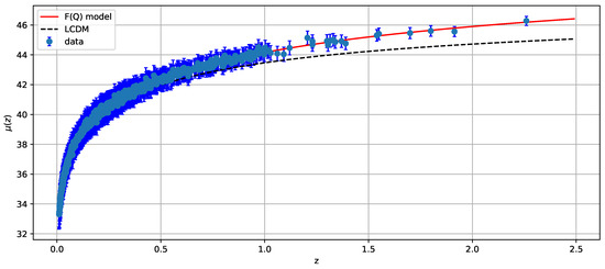
Figure 2.
The error bar plot of versus z for the considered model. The solid red line is the curve for the model, whereas the black dotted line represents the CDM model. The blue dots depict the 1048 points of the Pantheon data.
The and likelihood contours for the model parameters using the Hubble, BAO, and Pantheon datasets is presented in Figure 3. The obtained best-fit values are presented in Table 2.
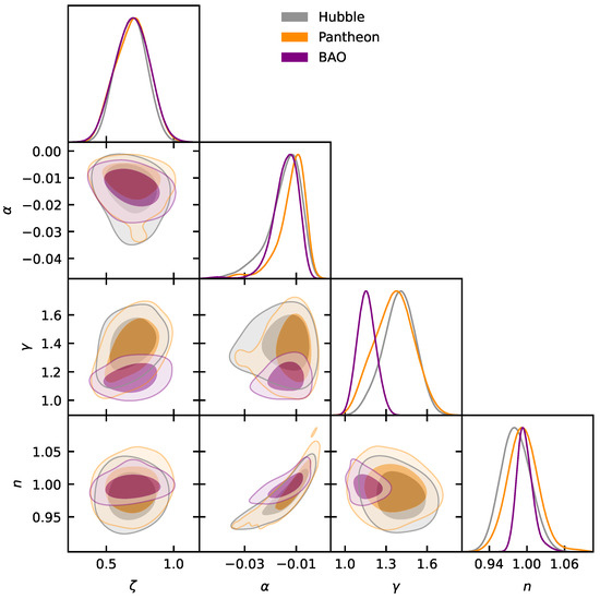
Figure 3.
The and likelihood contours for the model parameters using the Hubble, BAO, and the Pantheon datasets.
Table 2.
The table shows the constraints on the model parameters corresponding to the Hubble, BAO, and Pantheon datasets.
4.4. Cosmological Parameters
The evolution of the Hubble parameter, deceleration parameter, energy density, pressure with the bulk viscosity, and the effective EoS parameter for the redshift range are presented below, in order to test the late-time cosmic expansion history and the future of the expanding universe [101]. In order to do so, we used the set of values constrained by the Hubble, BAO, and Pantheon datasets for the model parameters.
From Figure 4, it is clear that the deceleration parameter shows the transition from a decelerated () to an accelerated () phase of the universe’s expansion for the constrained values of the model parameters. The transition redshift is , , and corresponding to the Hubble, BAO, and Pantheon datasets, respectively. The present value of the deceleration parameter is, respectively, , , and .
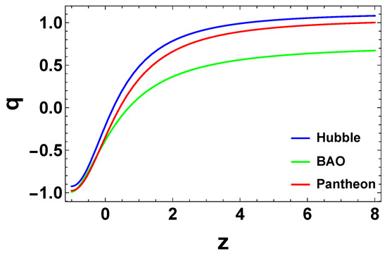
Figure 4.
Profile of the deceleration parameter for the given model corresponding to the values of the parameters constrained by the Hubble, BAO, and Pantheon data point sets.
From Figure 5 and Figure 6, it is clear that the Hubble and density parameters show the positive behavior for all the constrained values of the model parameters, which is expected.
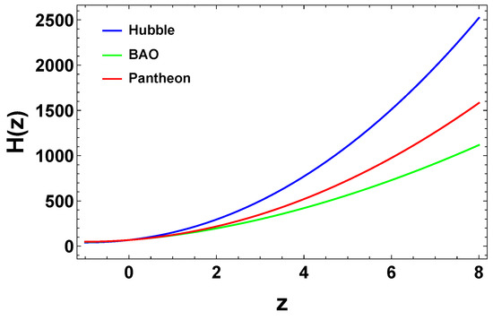
Figure 5.
Profile of the Hubble parameter for the given model corresponding to the values of the parameters constrained by the Hubble, BAO, and Pantheon data point sets.
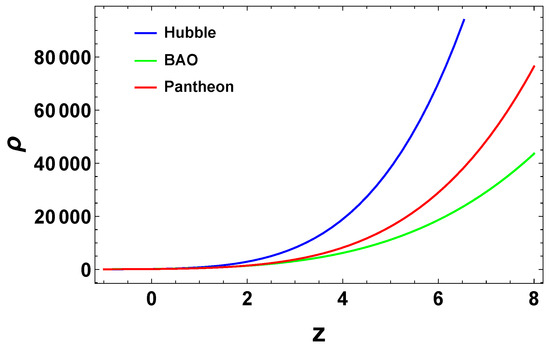
Figure 6.
Profile of the density parameter for the given model corresponding to the values of the parameters constrained by the Hubble, BAO, and Pantheon data point sets.
Figure 7 indicates that the bulk viscous cosmic fluid exhibits, for lower redshifts, the negative pressure that makes the bulk viscosity a viable candidate to drive the cosmic acceleration. Furthermore, the effective EoS parameter presented in Figure 8 indicates that the cosmic viscous fluid behaves like quintessence dark energy. The present values of the EoS parameter corresponding to the Hubble, BAO, and Pantheon samples are , , and .
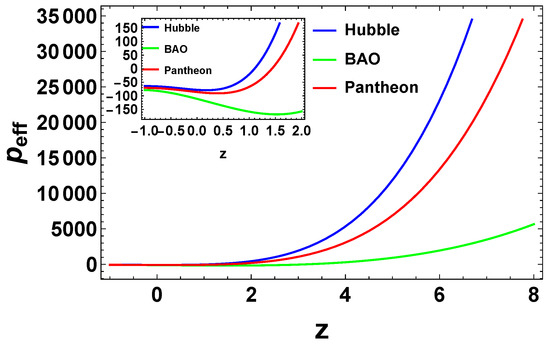
Figure 7.
Profile of the pressure for the given model corresponding to the values of the parameters constrained by the Hubble, BAO, and Pantheon data point sets.
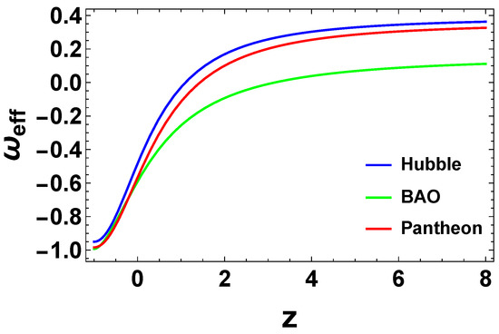
Figure 8.
Profile of the EoS parameter for the given model corresponding to the values of the parameters constrained by the Hubble, BAO, and Pantheon data point sets.
5. Energy Conditions
In the present section, we are going to construct the energy conditions for the solutions of the present model. The energy conditions are the relations applied to the matter energy–momentum tensor with the purpose of satisfying positive energy. The energy conditions are derived from the Raychaudhuri equation and are written as [102]:
- Null energy condition (NEC):;
- Weak energy condition (WEC): and ;
- Dominant energy condition (DEC):;
- Strong energy condition (SEC):.
with being the effective energy density.
In Figure 9 and Figure 10, it is evident that the NEC and DEC exhibit the positive behavior for all the constrained values of the model parameters. As the WEC is the combination of energy density and the NEC, we conclude that the NEC, DEC, and WEC are all satisfied in the entire domain of redshift. Figure 11 indicates that the SEC exhibits, for lower redshifts, the negative behavior that is related to cosmic acceleration [53,103]. This is also reflected in the deceleration parameter behavior in Figure 4.
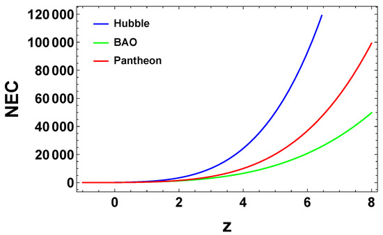
Figure 9.
Profile of the null energy condition for the given model corresponding to the values of the parameters constrained by the Hubble, BAO, and Pantheon data point sets.
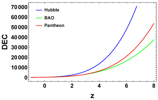
Figure 10.
Profile of the dominant energy condition for the given model corresponding to the values of the parameters constrained by the Hubble, BAO, and Pantheon data point sets.
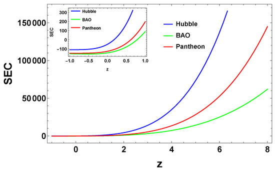
Figure 11.
Profile of the strong energy condition for the given model corresponding to the values of the parameters constrained by the Hubble, BAO, and Pantheon data point sets.
6. Statefinder Analysis
The cosmological constant suffers from two major drawbacks, namely the aforementioned cosmological constant and cosmic coincidence problems. To surmount these problems, dynamic models of dark energy have been introduced in the literature, as we have also mentioned in the Introduction. To discriminate between these time-varying dark energy models, an appropriate tool is required. In this direction, V. Sahni et al. introduced a new pair of geometrical parameters known as statefinder parameters [104]. The statefinder parameters are defined as
The parameter r can be rewritten as .
For different values of the statefinder pair , it represents the following dark energy models:
represents the CDM model;
represents the Chaplygin gas model;
represents the quintessence model.
In Figure 12 and Figure 13, we plot the and diagrams for our cosmological model by taking the values of the parameters constrained by the Hubble, BAO, and Pantheon datasets.
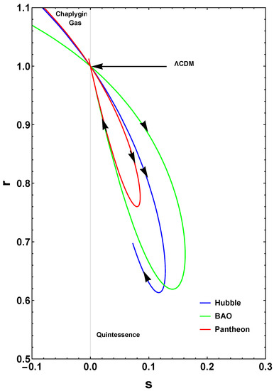
Figure 12.
Plot of the trajectories in the plane for the given cosmological model corresponding to the parameter values constrained by the Hubble, BAO, and Pantheon datasets.
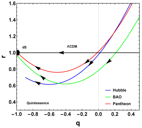
Figure 13.
Plot of the trajectories in the plane for the given cosmological model corresponding to the parameter values constrained by the Hubble, BAO, and the Pantheon datasets.
Figure 12 and Figure 13 show that our bulk viscous model lies in the quintessence region. Furthermore, the evolutionary trajectories of our model depart from the CDM point. The present values of the statefinder parameters corresponding to the values of the model parameters constrained by the Hubble, BAO, and Pantheon samples are and , and , and and , respectively.
7. Discussions and Conclusions
In the present section, we will discuss the results obtained in Section 4, Section 5 and Section 6 for the bulk viscous symmetric teleparallel cosmological model here developed and presented.
Cosmology has been on the agenda mainly for two reasons: dark energy and dark matter. While dark energy was deeply discussed throughout the paper, dark matter is predicted within the CDM model as a sort of matter that does not interact electromagnetically, so that it cannot be seen, but its gravitational effects otherwise can well be detected. Still, we have not yet detected or even associated dark matter with a particle of the standard model or beyond [105,106,107]. Modified (or alternative) theories of gravity have also been used to describe dark matter’s effects [108,109]. In these cases, dark matter is simply an effect of the modification of gravity.
Returning to the dark energy question, it is highly counter-intuitive that the expansion of the universe is actually accelerating. Although the vacuum quantum energy can well explain this dynamical effect via the cosmological constant in Einstein’s field equations of GR, the aforementioned important and persistent problems related to supply the search for alternative explanations.
In the present article, as an attempt to describe dark energy, we assumed the symmetric teleparallel gravity as the underlying gravity theory.
The gravity was recently proposed by Jiménez et al. in [31] as a ramification of the geometric trinity, which says that the spacetime manifold can be described by curvature, torsion, or non-metricity. In particular the symmetric teleparallel gravity describes gravitational interactions via the non-metricity scalar, with null curvature and torsion.
Our cosmological model was based on a spatially homogeneous and isotropic flat metric and an energy–momentum tensor describing a bulk viscous fluid. We let the function be a power of n as , with n a free parameter.
In Section 4, we started testing our cosmological solutions. We started confronting the Hubble parameter (30) with 31 data points that are measured from the differential age approach.We then plotted Figure 1 and Figure 2, in which and for our model are confronted with cosmological data and compared with the CDM prediction. We can see the model describes observations with good agreement, and it is clear that it provides a better fit when compared to the CDM model. Further, in Figure 3, we obtained the best-fit values for the model free parameters presented in Table 2.
From Figure 5 and Figure 6, we found that the Hubble and density parameters show the expected positive behavior for all the constrained values of the model parameters. Figure 7 indicates that the bulk viscous cosmic fluid exhibits the negative pressure that makes the bulk viscosity a viable candidate to drive the cosmic acceleration. This is also reflected in the deceleration parameter behavior in Figure 4, which shows a transition from decelerated to accelerated phases of the universe’s expansion. Furthermore, the effective EoS parameter presented in Figure 8 indicates that the cosmic viscous fluid behaves like quintessence dark energy.
In Section 5, we investigated the consistency of our model by analyzing the different energy conditions. We found that the NEC, DEC, and WEC are all satisfied in the entire domain of redshift (presented in Figure 9 and Figure 10), while the SEC, presented in Figure 11, is violated for lower redshifts, which implies the cosmic acceleration, and satisfied for higher redshifts, which implies a decelerated phase of the universe.
In Section 6, Figure 12 and Figure 13 show that the evolutionary trajectories of our model depart from the CDM fixed point . In the present epoch, they lie in the quintessence region . The present model is, therefore, a good alternative to explain the universe’s dynamics, particularly with no necessity of invoking the cosmological constant.
Author Contributions
Conceptualization, R.S.; Data curation, R.S. and S.A.; Formal analysis, P.H.R.S.M. and P.K.S.; Investigation, R.S. and S.A.; Methodology, R.S. and S.A.; Project administration, P.K.S.; Software, R.S. and S.A.; Supervision, P.H.R.S.M. and P.K.S.; Validation, P.H.R.S.M. and P.K.S.; Visualization, R.S. and S.A.; Writing—original draft, R.S. and S.A.; Writing—review & editing, P.H.R.S.M. and P.K.S. All authors have read and agreed to the published version of the manuscript.
Funding
This research received no external funding.
Institutional Review Board Statement
Not applicable.
Informed Consent Statement
Not applicable.
Data Availability Statement
There are no new data associated with this article.
Acknowledgments
RS acknowledges University Grants Commission (UGC), New Delhi, India for awarding Junior Research Fellowship (UGC-Ref. No.: 191620096030). SA acknowledges CSIR, New Delhi, India for SRF. PKS acknowledges CSIR, New Delhi, India for financial support to carry out the Research project [No.03(1454)/19/EMR-II Dt.02/08/2019] and IUCAA, Pune, India for providing support through visiting associateship program. We are very much grateful to the honorable referees and to the editor for the illuminating suggestions that have significantly improved our work in terms of research quality, and presentation.
Conflicts of Interest
The authors declare no conflict of interest.
References
- Riess, A.G.; Filippenko, A.V.; Challis, P.; Clocchiatti, A.; Diercks, A.; Garnavich, P.M.; Gilliland, R.L.; Hogan, C.J.; Jha, S.; Kirshner, R.P.; et al. Observational Evidence from Supernovae for an Accelerating Universe and a Cosmological Constant. Astron. J. 1998, 116, 1009. [Google Scholar] [CrossRef]
- Perlmutter, S.; Aldering, G.; Goldhaber, G.; Knop, R.A.; Nugent, P.; Castro, P.G.; Deustua, S.; Fabbro, S.; Goobar, A.; Groom, D.E.; et al. Measurements of Ω and Λ from 42 High-Redshift Supernovae. Astrophys. J. 1999, 517, 565. [Google Scholar] [CrossRef]
- Koivisto, T.; Mota, D.F. Dark energy anisotropic stress and large scale structure formation. Phys. Rev. D 2006, 73, 083502. [Google Scholar] [CrossRef]
- Daniel, S.F. Large scale structure as a probe of gravitational slip. Phys. Rev. D 2008, 77, 103513. [Google Scholar] [CrossRef]
- Eisenstein, D.J.; Zehavi, I.; Hogg, D.W.; Scoccimarro, R.; Blanton, M.R.; Nichol, R.C.; Scranton, R.; Seo, H.-J.; Tegmark, M.; Zheng, Z.; et al. Detection of the Baryon Acoustic Peak in the Large-Scale Correlation Function of SDSS Luminous Red Galaxies. Astrophys. J. 2005, 633, 560. [Google Scholar] [CrossRef]
- Percival, W.J.; Reid, B.A.; Eisenstein, D.J.; Bahcall, N.A.; Budavari, T.; Frieman, J.A.; Fukugita, M.; Gunn, J.E.; Ivezic, Z.; Knapp, G.R.; et al. Baryon acoustic oscillations in the Sloan Digital Sky Survey Data Release 7 galaxy sample. Mon. Not. R. Astron. Soc. 2010, 401, 2148–2168. [Google Scholar] [CrossRef]
- Caldwell, R.R.; Doran, M. Cosmic microwave background and supernova constraints on quintessence: Concordance regions and target models. Phys. Rev. D 2004, 69, 103517. [Google Scholar] [CrossRef]
- Huang, Z.Y.; Wang, B.; Abdalla, E.; Suet, R.K. Holographic explanation of wide-angle power correlation suppression in the cosmic microwave background radiation. J. Cosm. Astrop. Phys. 2006, 0605, 013. [Google Scholar] [CrossRef]
- Dalal, N.; Abazajian, K.; Jenkins, E.; Manoharet, A.V. Testing the Cosmic Coincidence Problem and the Nature of Dark Energy. Phys. Rev. Lett. 2001, 87, 141302. [Google Scholar] [CrossRef]
- Weinberg, S. The cosmological constant problem. Rev. Mod. Phys. 1989, 61, 1. [Google Scholar] [CrossRef]
- Bento, M.C.; Bertolami, O.; Sen, A.A. Generalized Chaplygin gas, accelerated expansion, and dark-energy-matter unification. Phys. Rev. D 2002, 66, 043507. [Google Scholar] [CrossRef]
- Kamenshchik, A.Y.; Moschella, U.; Pasquier, V. An alternative to quintessence. Phys. Lett. B 2001, 511, 265. [Google Scholar] [CrossRef]
- Chiba, T.; Okabe, T.; Yamaguchi, M. Kinetically driven quintessence. Phys. Rev. D 2000, 62, 023511. [Google Scholar] [CrossRef]
- Armendariz-Picon, C.; Mukhanov, V.; Steinhardt, P.J. Dynamical Solution to the Problem of a Small Cosmological Constant and Late-Time Cosmic Acceleration. Phys. Rev. Lett. 2000, 85, 4438. [Google Scholar] [CrossRef]
- Carroll, S.M. Quintessence and the Rest of the World: Suppressing Long-Range Interactions. Phys. Rev. Lett. 1998, 81, 3067. [Google Scholar] [CrossRef]
- Fujii, Y. Origin of the gravitational constant and particle masses in a scale-invariant scalar-tensor theory. Phys. Rev. D 1982, 26, 2580. [Google Scholar] [CrossRef]
- Xu, L.; Wang, Y.; Tong, M.; Noh, H. CMB temperature and matter power spectrum in a decay vacuum dark energy model. Phys. Rev. D 2011, 84, 123004. [Google Scholar] [CrossRef]
- Tong, M.; Noh, H. Observational constraints on decaying vacuum dark energy model. Eur. Phys. J. C 2011, 71, 1586. [Google Scholar] [CrossRef]
- Freese, K.; Adams, F.C.; Frieman, J.A.; Mottola, E. Cosmology with decaying vacuum energy. Nucl. Phys. B 1987, 287, 797. [Google Scholar] [CrossRef]
- Abdel-Rahman, A.-M.M. Nonsingular decaying-vacuum cosmology and baryonic matter. Phys. Rev. D 1992, 45, 3497. [Google Scholar] [CrossRef]
- Appleby, S.; Battye, R. Do consistent F(R) models mimic General Relativity plus Λ. Phys. Lett. B 2007, 654, 7. [Google Scholar] [CrossRef]
- Amendola, L.; Gannouji, R.; Polarski, D.; Tsujikawa, S. Conditions for the cosmological viability of f(R) dark energy models. Phys. Rev. D 2007, 75, 083504. [Google Scholar] [CrossRef]
- Saffari, R.; Rahvar, S. f(R) gravity: From the Pioneer anomaly to cosmic acceleration. Phys. Rev. D 2008, 77, 104028. [Google Scholar] [CrossRef]
- Cognola, G.; Elizalde, E.; Nojiri, S.; Odintsov, S.D.; Zerbini, S. Dark energy in modified Gauss-Bonnet gravity: Late-time acceleration and the hierarchy problem. Phys. Rev. D 2006, 73, 084007. [Google Scholar] [CrossRef]
- Li, B.; Barrow, J.D.; Mota, D.F. Cosmology of modified Gauss-Bonnet gravity. Phys. Rev. D 2007, 76, 044027. [Google Scholar] [CrossRef]
- Moraes, P.H.R.S.; Santos, J.R.L. A complete cosmological scenario from f(R,Tϕ) gravity theory. Eur. Phys. J. C 2016, 76, 60. [Google Scholar]
- Ren, X.; Wong, T.H.T.; Cai, Y.F.; Saridakis, E.N. Data-driven Reconstruction of the Late-time Cosmic Acceleration with f(T) Gravity. Phys. Dark Univ. 2021, 32, 100812. [Google Scholar] [CrossRef]
- Nashed, G.L.; Capozziello, S. Charged Anti-de Sitter BTZ black holes in Maxwell-f(T) gravity. Gen. Rel. Grav. 2015, 47, 75. [Google Scholar] [CrossRef]
- Setare, M.R.; Mohammadipour, N. Can f(T) gravity theories mimic ΛCDM cosmic history. J. Cosm. Astrop. Phys. 2013, 01, 015. [Google Scholar] [CrossRef]
- Bahamonde, S.; Dialektopoulos, K.; Escamilla-Rivera, C.; Farrugia, G.; Gakis, V.; Hendry, M.; Hohmann, M.; Said, J.; Mifsud, J.; Valentino, E.D. Teleparallel Gravity: From Theory to Cosmology. arXiv 2021, arXiv:2106.13793. [Google Scholar] [CrossRef]
- Jiménez, J.B.; Heisenberg, L.; Koivisto, T. Coincident general relativity. Phys. Rev. D 2018, 98, 044048. [Google Scholar] [CrossRef]
- Hehl, F.W.; McCrea, J.D.; Mielke, E.W.; Neéman, Y. Metric-affine gauge theory of gravity: Field equations, Noether identities, world spinors, and breaking of dilation invariance. Phys. Rep. 1995, 258, 1–171. [Google Scholar] [CrossRef]
- Hehl, F.W.; Neéman, Y.; Nitsch, J.; Heyde, P.V.D. Short-range confining component in a quadratic poincare gauge theory of gravitation. Phys. Lett. B 1978, 78, 102–106. [Google Scholar] [CrossRef]
- Hehl, F.W.; Obukhov, Y.N. How does the electromagnetic field couple to gravity, in particular to metric, nonmetricity, torsion, and curvature ? arXiv 2000, arXiv:0001010. [Google Scholar]
- Ne’eman, Y.; Hehl, F.W. Matter Particled—Patterns, Structure and Dynamics. Class. Quant. Grav. 1997, 14, 251–260. [Google Scholar]
- Nester, J.M.; Yo, H.-J. Symmetric teleparallel general relativity. Chin. J. Phys. 1999, 37, 113. [Google Scholar]
- Boulanger, N.; Kirsch, I. Higgs mechanism for gravity. II. Higher spin connections Phys. Rev. D 2006, 73, 124023. [Google Scholar]
- Baekler, P.; Boulanger, N.; Hehl, F.W. Linear connections with a propagating spin-3 field in gravity. Phys. Rev. D 2006, 74, 125009. [Google Scholar] [CrossRef]
- Weyl, H. Gravitation and electricity. Sitzungsber. Preuss. Akad. Wiss. 1918, 465, 1. [Google Scholar] [CrossRef]
- Dialektopoulos, K.F.; Koivisto, T.S.; Capozziello, S. Noether symmetries in symmetric teleparallel cosmology. Eur. Phys. J. C 2019, 79, 606. [Google Scholar] [CrossRef]
- Frusciante, N. Signatures of f(Q) gravity in cosmology. Phys. Rev. D 2021, 103, 044021. [Google Scholar] [CrossRef]
- Barros, B.J.; Barreiro, T.; Koivisto, T.; Nunes, N.J. Testing F(Q) gravity with redshift space distortions. Phys. Dark Univ. 2020, 30, 100616. [Google Scholar] [CrossRef]
- Ferreira, J.; Barreiro, T.; Mimoso, J.; Nunes, N.J. Forecasting F(Q) cosmology with ΛCDM background using standard sirens. Phys. Rev. D 2022, 105, 123531. [Google Scholar] [CrossRef]
- Albuquerque, I.S.; Frusciante, N. A designer approach to f(Q) gravity and cosmological implications. Phys. Dark Univ. 2022, 35, 100980. [Google Scholar] [CrossRef]
- Capozziello, S.; D’Agostino, R. Model-independent reconstruction of f(Q) non-metric gravity. Phys. Lett. B 2022, 832, 137229. [Google Scholar] [CrossRef]
- Atayde, L.; Frusciante, N. Can f(Q) gravity challenge ΛCDM . Phys. Rev. D 2022, 104, 064052. [Google Scholar] [CrossRef]
- Ayuso, I.; Lazkoz, R.; Salzano, V. Observational constraints on cosmological solutions of f(Q) theories. Phys. Rev. D 2021, 103, 063505. [Google Scholar] [CrossRef]
- Khyllep, W. Cosmology in f(Q) gravity: A unified dynamical system analysis at background and perturbation levels. arXiv 2022, arXiv:2207.02610. [Google Scholar]
- Sahlu, S.; Tsegaye, E. Linear Cosmological perturbations in F(Q) Gravity. arXiv 2022, arXiv:2206.02517. [Google Scholar]
- Jiménez, J.B.; Heisenberg, L.; Koivisto, T.; Pekar, S. Cosmology in f(Q) geometry. Phys. Rev. D 2020, 101, 103507. [Google Scholar] [CrossRef]
- Khyllep, W.; Paliathanasis, A.; Dutta, J. Cosmological solutions and growth index of matter perturbations in f(Q) gravity. Phys. Rev. D 2021, 103, 103521. [Google Scholar] [CrossRef]
- Mandal, S.; Wang, D.; Sahoo, P.K. Cosmography in f(Q) gravity. Phys. Rev. D 2020, 102, 124029. [Google Scholar] [CrossRef]
- Mandal, S.; Sahoo, P.K.; Santos, J.R.L. Energy conditions in f(Q) gravity. Phys. Rev. D 2020, 102, 024057. [Google Scholar] [CrossRef]
- Wilson, J.R.; Mathews, G.J.; Fuller, G.M. Bulk viscosity, decaying dark matter, and the cosmic acceleration. Phys. Rev. D 2007, 75, 043521. [Google Scholar] [CrossRef]
- Okumura, H.; Yonezawa, F. New expression of the bulk viscosity. Phys. A 2003, 321, 207. [Google Scholar] [CrossRef]
- Bali, R.; Jain, D.R. Some expanding and shearing viscous fluid cosmological models in general relativity. Astrophys. Spa. Sci. 1988, 141, 207. [Google Scholar] [CrossRef]
- Bali, R.; Jain, D.R. A gravitationally non-degenerate cosmological model with expanding and shearing viscous fluid in general relativity. Astriphys. Spa. Sci. 1987, 139, 175. [Google Scholar] [CrossRef]
- Deng, Y.; Mannheim, P.D. Acceleration-free spherically symmetric inhomogeneous cosmological model with shear viscosity. Phys. Rev. D 1991, 44, 1722. [Google Scholar] [CrossRef]
- Huang, W.-H. Effects of the shear viscosity on the character of cosmological evolution. J. Math. Phys. 1990, 31, 659. [Google Scholar] [CrossRef]
- Samanta, G.C.; Myrzakulov, R.; Shah, P. Kaluza–Klein Bulk Viscous Fluid Cosmological Models and the Validity of the Second Law of Thermodynamics in f(R,T) Gravity. Zeits. Naturfor. 2017, 72, 365. [Google Scholar] [CrossRef]
- Satish, J.; Venkateswarlu, R. Bulk viscous fluid cosmological models in f(R, T) gravity. Chin. J. Phys. 2016, 54, 830. [Google Scholar]
- Beesham, A. Cosmological Models with a Variable Cosmological Term and Bulk Viscous Models. Phys. Rev. D 1993, 48, 3539. [Google Scholar] [CrossRef] [PubMed]
- Colistete, R., Jr.; Fabris, J.C.; Tossa, J.; Zimdahl, W. Bulk viscous cosmology. Phys. Rev. D 2007, 76, 103516. [Google Scholar] [CrossRef]
- Sadatian, S.D. Effects of viscous content on the modified cosmological F(T) model. EPL 2019, 126, 30004. [Google Scholar] [CrossRef]
- Brevik, I. Viscosity in Modified Gravity. Entropy 2012, 14, 2302–2310. [Google Scholar] [CrossRef]
- Singh, C.P.; Kumar, P. Friedmann model with viscous cosmology in modified f(R,T) gravity theory. Eur. Phys. J. C 2014, 74, 3070. [Google Scholar] [CrossRef]
- Srivastava, M.; Singh, C.P. New holographic dark energy model with constant bulk viscosity in modified f(R,T) gravity theory. Astrophys. Space Sci. 2018, 363, 117. [Google Scholar] [CrossRef]
- Paolis, F.D.; Jamil, M.; Qadir, A. Black holes in bulk viscous cosmology. Int. J. Theor. Phys. 2010, 49, 621–632. [Google Scholar] [CrossRef]
- Brevik, I.; Jamil, M. Black holes in the turbulence phase of viscous rip cosmology. Int. J. Geom. Meth. Mod. Phys. 2019, 16, 1950030. [Google Scholar] [CrossRef]
- Jimenez, R.; Loeb, A. Constraining cosmological parameters based on relative galaxy ages. ApJ 2002, 573, 37. [Google Scholar] [CrossRef]
- Sharov, G.S.; Bhattacharya, S.; Pan, S.; Nunes, R.C.; Chakraborty, S. A new interacting two-fluid model and its consequences. Mon. Not. R. Astron. Soc. 2017, 466, 3497. [Google Scholar] [CrossRef]
- Blake, C.; Kazin, E.A.; Beutler, F.; Davis, T.M.; Parkinson, D.; Brough, S.; Colless, M.; Contreras, C.; Couch, W.; Croom, S.; et al. The WiggleZ Dark Energy Survey: Mapping the distance-redshift relation with baryon acoustic oscillations. Mon. Not. R. Astron. Soc. 2011, 418, 1707. [Google Scholar] [CrossRef]
- Scolnic, D.M.; Jones, D.O.; Rest, A.; Pan, Y.C.; Chornock, R.; Foley, R.J.; Huber, M.E.; Kessler, R.; Narayan, G.; Riess, A.G.; et al. The complete light-curve sample of spectroscopically confirmed SNe Ia from Pan-STARRS1 and cosmological constraints from the combined pantheon sample. ApJ 2018, 859, 101. [Google Scholar] [CrossRef]
- Lazkoz, R.; Lobo, F.S.N.; Ortiz-Banos, M.; Salzano, V. Observational constraints of f(Q) gravity. Phys. Rev. D 2019, 100, 104027. [Google Scholar] [CrossRef]
- Beh, J.T.; Loo, T.H.; De, A. Geodesic Deviation Equation In f(Q) Gravity. arXiv 2021, arXiv:2107.04513. [Google Scholar] [CrossRef]
- Dimakis, N.; Paliathanasis, A.; Christodoulakis, T. Quantum Cosmology in f(Q) theory. arXiv 2021, arXiv:2108.01970. [Google Scholar] [CrossRef]
- Maluf, J.W. The teleparallel equivalent of general relativity. Ann. Phys. 2013, 525, 339. [Google Scholar] [CrossRef]
- Hohmann, M. General covariant symmetric teleparallel cosmology. Phys. Rev. D 2021, 104, 124077. [Google Scholar] [CrossRef]
- Vagnozzi, S.; Loeb, A.; Moresco, M. The cosmic chronometers take on spatial curvature and cosmic concordance. Astrophys. J. 2021, 908, 84. [Google Scholar]
- Gusakov, M.E. Bulk viscosity of superfluid neutron stars. Phys. Rev. D 2007, 76, 083001. [Google Scholar] [CrossRef]
- Gusakov, M.E.; Kantor, E.M. Bulk viscosity of superfluid hyperon stars. Phys. Rev. D 2008, 78, 083006. [Google Scholar] [CrossRef]
- Haensel, P.; Levenfish, K.P.; Yakovlev, D.G. Bulk viscosity in superfluid neutron star cores-III. Effects of hyperons. Astron. Astrophys. 2002, 381, 1080. [Google Scholar] [CrossRef]
- Ryden, B. Introduction to Cosmology; Addison Wesley: San Francisco, CA, USA, 2003. [Google Scholar]
- Odintsov, S.D.; Gomez, D.S.C.; Sharov, G.S. Testing the equation of state for viscous dark energy. Phys. Rev. D 2020, 101, 044010. [Google Scholar] [CrossRef]
- Fabris, J.C.; Goncalves, S.V.B.; Ribeiro, R. Bulk viscosity driving the acceleration of the Universe. Gen. Rel. Grav. 2006, 38, 495. [Google Scholar] [CrossRef]
- Meng, X.-H.; Dou, X. Friedmann cosmology with bulk viscosity: A concrete model for dark energy. Comm. Theor. Phys. 2009, 52, 377. [Google Scholar]
- Brevik, I.; Gorbunova, O. Dark energy and viscous cosmology. Gen. Rel. Grav. 2005, 37, 2039. [Google Scholar] [CrossRef]
- Gron, O. Viscous inflationary universe models. Astrophys. Space Sci. 1990, 173, 191–225. [Google Scholar] [CrossRef]
- Eckart, C. The thermodynamics of irreversible processes. III. Relativistic theory of the simple fluid Phys. Rev. 1940, 58, 919. [Google Scholar]
- Ren, J.; Meng, X.-H. Cosmological model with viscosity media (dark fluid) described by an effective equation of state. Phys. Lett. B 2006, 633, 1–8. [Google Scholar] [CrossRef]
- Harko, T.; Koivisto, T.S.; Lobo, F.S.N.; Olmo, G.J.; Rubiera-Garcia, D. Coupling matter in modified Q gravity. Phys. Rev. D 2018, 98, 084043. [Google Scholar] [CrossRef]
- Mackey, D.F.; Hogg, D.W.; Lang, D.; Goodman, J. emcee: The MCMC hammer. Publ. Astron. Soc. Pac. 2013, 125, 306. [Google Scholar] [CrossRef]
- Sharov, G.S.; Vasilie, V.O. How predictions of cosmological models depend on Hubble parameter data sets. Math. Model. Geom. 2018, 6, 1. [Google Scholar] [CrossRef]
- Beutler, F.; Blake, C.; Colless, M.; Jones, D.H.; Staveley-Smith, L.; Campbell, L.; Parker, Q.; Saunders, W.; Watson, F. The 6dF Galaxy Survey: Baryon acoustic oscillations and the local Hubble constant. Mon. Not. R. Astron. Soc. 2011, 416, 3017. [Google Scholar] [CrossRef]
- Jarosik, N.; Bennett, C.L.; Dunkley, J.; Gold, B.; Greason, M.R.; Halpern, M.; Hill, R.S.; Hinshaw, G.; Kogut, A.; Komatsu, E. SEVEN-YEAR WILKINSON MICROWAVE ANISOTROPY PROBE (WMAP) OBSERVATIONS: SKY MAPS, SYSTEMATIC ERRORS, AND BASIC RESULTS. Astrophys. J. Suppl. 2011, 192, 14. [Google Scholar] [CrossRef]
- Giostri, R.; Santos, M.V.d.; Waga, I.; Reis, R.R.R.; Calvao, M.O.; Lago, B.L. From cosmic deceleration to acceleration: New constraints from SN Ia and BAO/CMB. J. Cosm. Astropart. Phys. 2012, 03, 027. [Google Scholar] [CrossRef]
- Mukherjee, P.; Banerjee, N. Non-parametric reconstruction of the cosmological jerk parameter. Eur. Phys. J. C 2021, 81, 36. [Google Scholar] [CrossRef]
- Tripp, R. A two-parameter luminosity correction for Type IA supernovae. Astron. Astrophys. 1998, 331, 815. [Google Scholar]
- Kessler, R.; Scolnic, D. Correcting type Ia supernova distances for selection biases and contamination in photometrically identified samples. Astrophys. J. 2017, 836, 56. [Google Scholar] [CrossRef]
- Anagnostopoulos, F.K.; Basilakos, S.; Saridakis, E.N. Observational constraints on Myrzakulov gravity. Phys. Rev. D 2021, 103, 104013. [Google Scholar] [CrossRef]
- Vagnozzi, S.; Pacucci, F.; Loeb, A. Implications for the Hubble tension from the ages of the oldest astrophysical objects. JHEAp 2022, 36, 27–35. [Google Scholar] [CrossRef]
- Raychaudhuri, A. Relativistic cosmology I. Phys. Rev. 1955, 98, 1123. [Google Scholar] [CrossRef]
- Capozziello, S.; Lobo, F.S.N.; Mimoso, J.O. Energy conditions in modified gravity. Phys. Lett. B 2014, 730, 280–283. [Google Scholar] [CrossRef]
- Sahni, V.; Saini, T.D.; Starobinsky, A.A.; Alam, U. Statefinder-a new geometrical diagnostic of dark energy. JETP Lett. 2003, 77, 201. [Google Scholar] [CrossRef]
- CDMS II Collaboration. Science 2010, 327, 1619.
- Akerib, D.S.; Araujo, H.M.; Bai, X.; Bailey, A.J.; Balajthy, J.; Bedikian, S.; Bernard, E.; Bernstein, A.; Bolozdynya, A.; Bradley, A.; et al. First Results from the LUX Dark Matter Experiment at the Sanford Underground Research Facility. Phys. Rev. Lett. 2014, 112, 091303. [Google Scholar] [CrossRef] [PubMed]
- Essig, R.; Manalaysay, A.; Mardon, J.; Sorensen, P.; Volansky, T. First direct detection limits on sub-GeV dark matter from XENON10. Phys. Rev. Lett 2012, 109, 021301. [Google Scholar] [CrossRef] [PubMed]
- Bohmer, C.G.; Harko, T.; Lobo, F.S.N. Dark matter as a geometric effect in f(R) gravity. Astrop. Phys. 2008, 29, 386. [Google Scholar] [CrossRef]
- Mannheim, P.D.; O’Brien, J.G. Fitting galactic rotation curves with conformal gravity and a global quadratic potential. Phys. Rev. D 2012, 85, 124020. [Google Scholar] [CrossRef]


Disclaimer/Publisher’s Note: The statements, opinions and data contained in all publications are solely those of the individual author(s) and contributor(s) and not of MDPI and/or the editor(s). MDPI and/or the editor(s) disclaim responsibility for any injury to people or property resulting from any ideas, methods, instructions or products referred to in the content. |
© 2022 by the authors. Licensee MDPI, Basel, Switzerland. This article is an open access article distributed under the terms and conditions of the Creative Commons Attribution (CC BY) license (https://creativecommons.org/licenses/by/4.0/).