
The Classification of Blazar Candidates of Uncertain Types


 , and
, and
Abstract
:1. Introduction
2. Sample and Classifications
2.1. Samples
2.2. Average Values
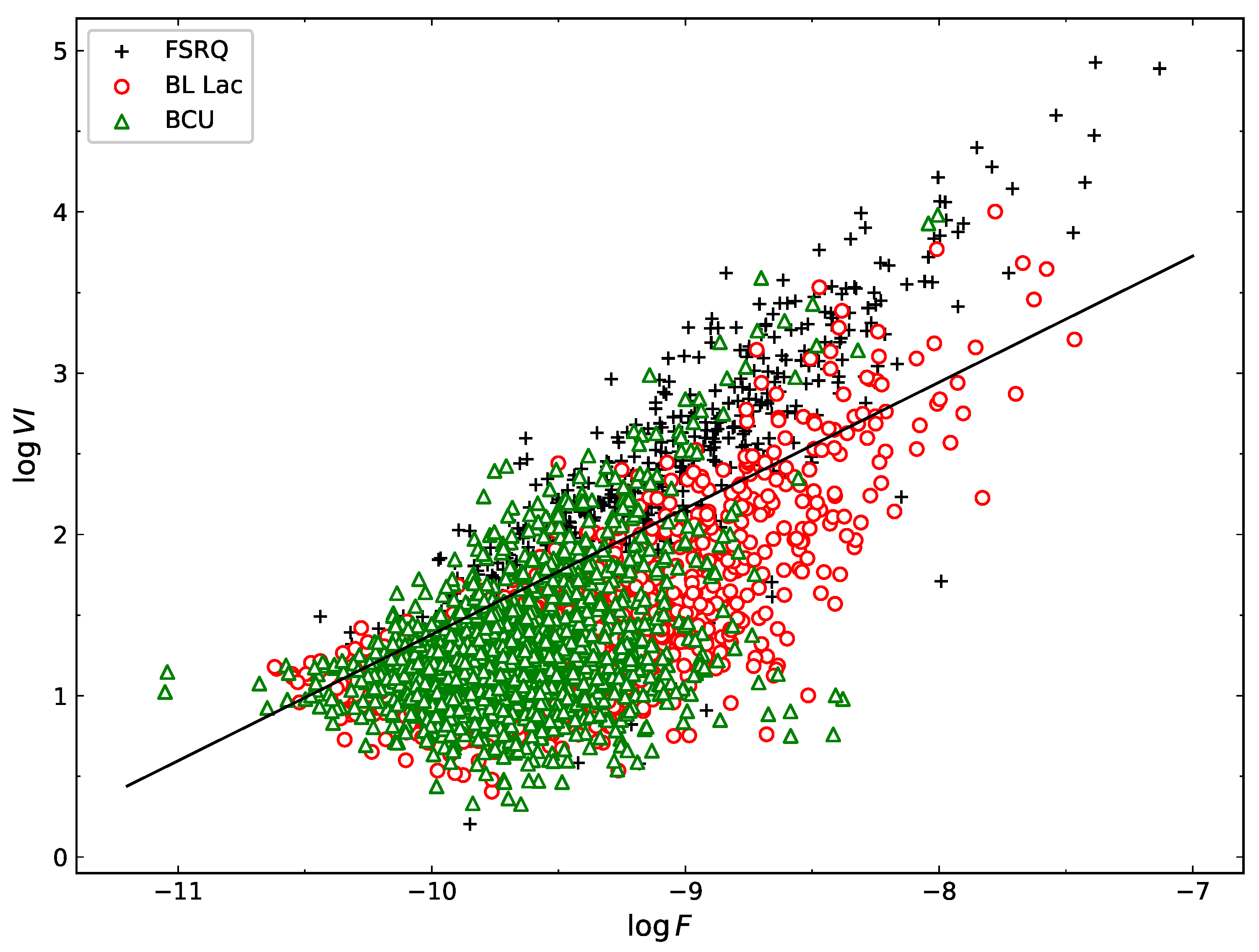
2.3. Correlations
2.4. Classifications
3. Discussions
3.1. The Average Values
3.2. The Correlations for FSRQs and BL Lacs
3.3. The Classification for BCUs
4. Conclusions
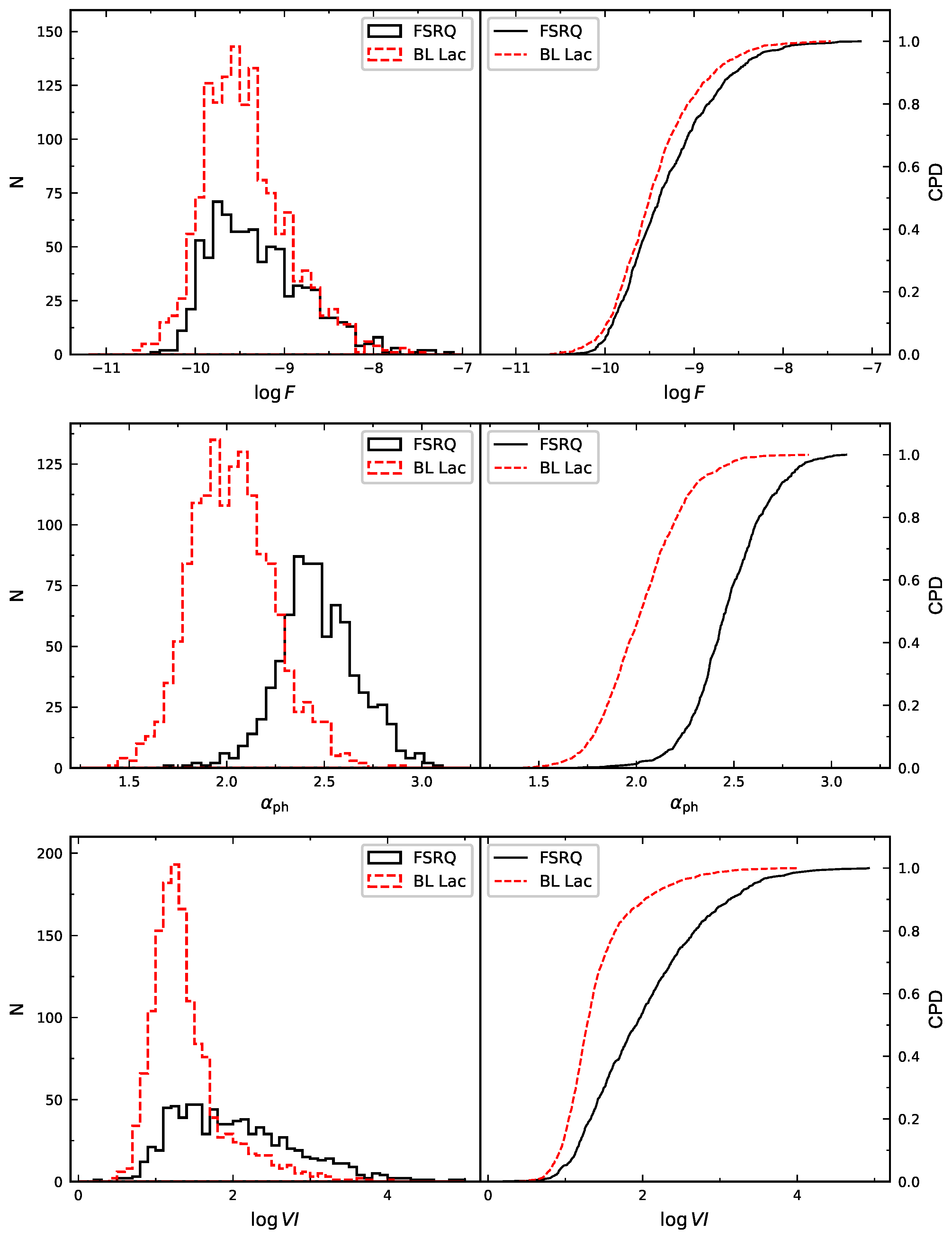
- The -ray photon flux, spectral index and variability index of FSRQs were higher than those of BL Lacs for the known blazar sample. There is a sequence from FSRQs to LBLs to HBLs that is similar to that in Fossati et al. [39].
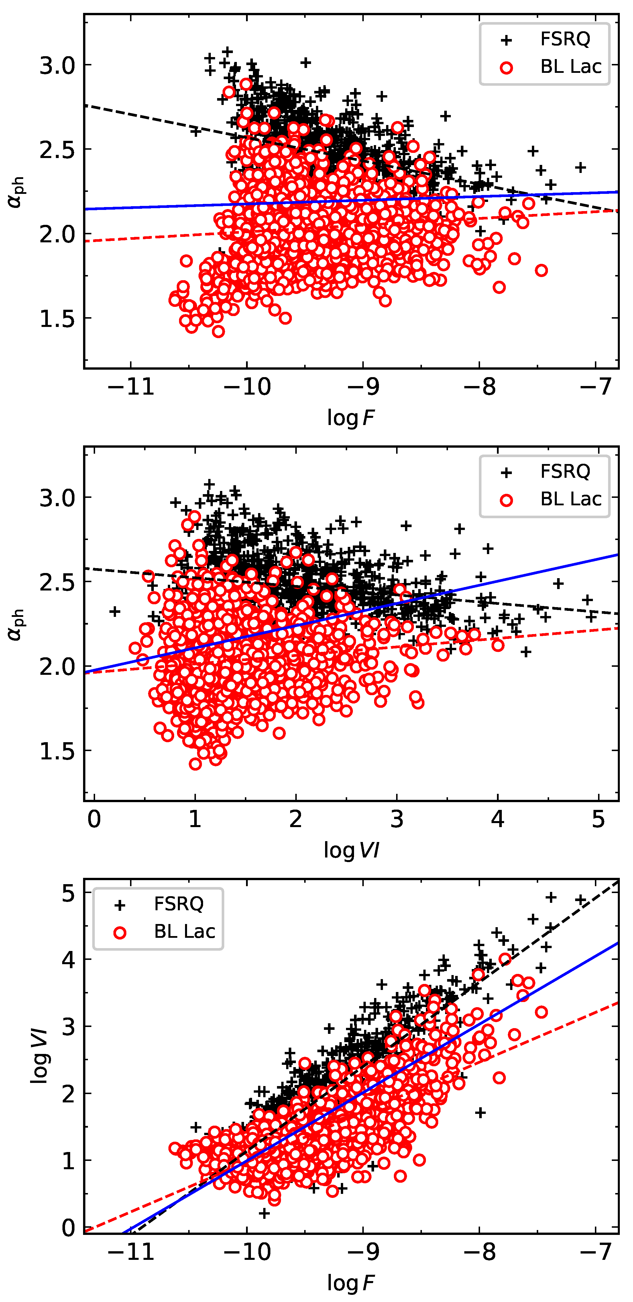
- A positive correlation was found between the -ray flux and the photon spectral index for the whole sample; however, an anti-correlation was found for FSRQs and a positive correlation for BL Lacs. In addition, a positive correlation was found between the variability index () and the -ray photon spectrum index () for the whole sample but an anti-correlation for FSRQs and a positive correlation for BL Lacs. We found that those two positive correlations for the whole sample were apparent.
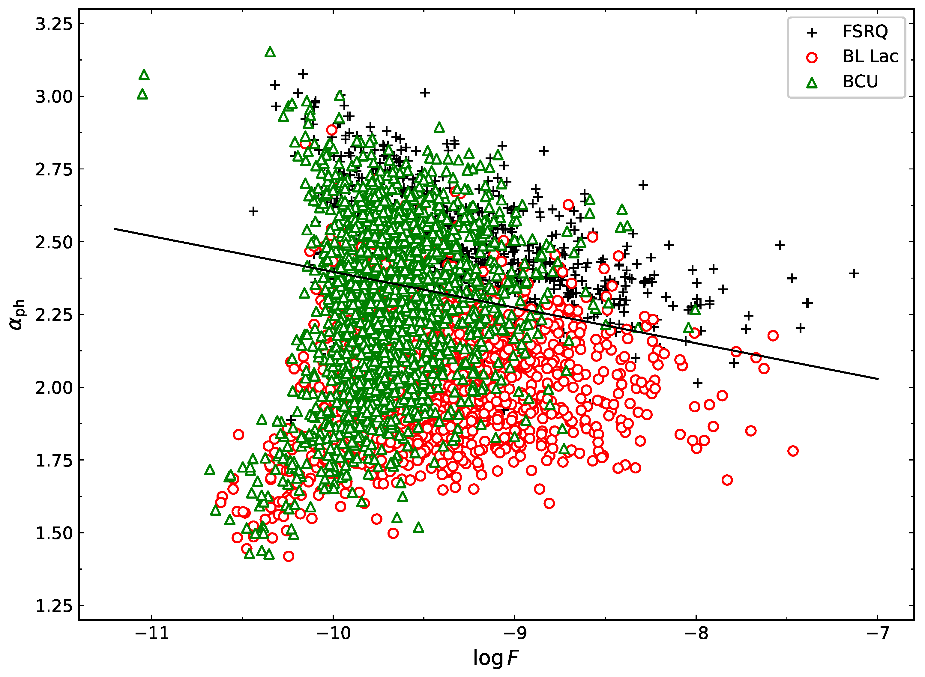
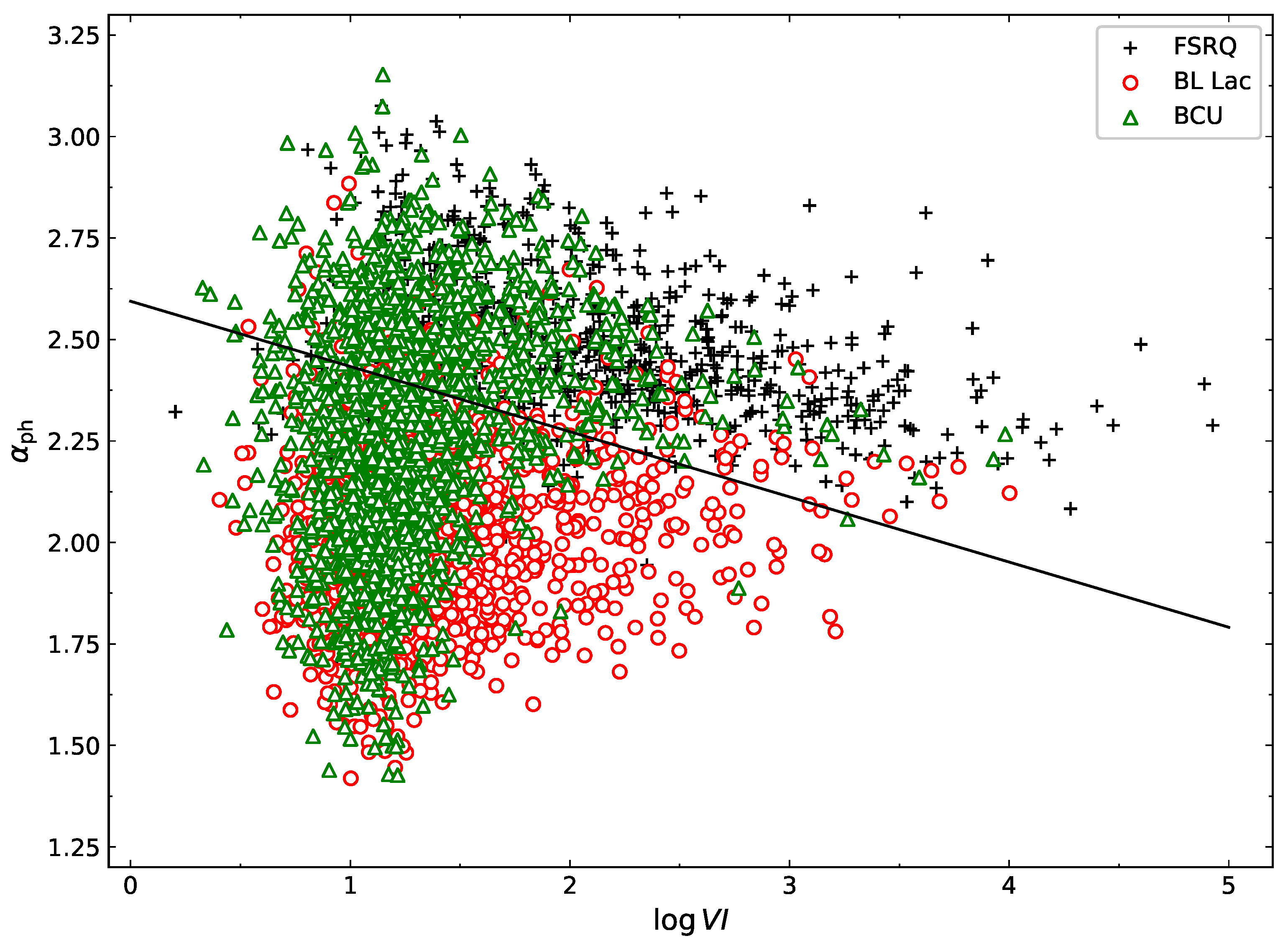
- We adopted the SVM machine-learning method to classify BL Lacs and FSRQs in the , and plots and . We obtained 932 BL Lac candidates and possible BL Lac candidates as well as 585 FSRQ candidates and possible FSRQ candidates.
Author Contributions
Funding
Institutional Review Board Statement
Data Availability Statement
Acknowledgments
Conflicts of Interest
References
- Abdollahi, S.; Acero, F.; Ackermann, M.; Ajello, M.; Atwood, W.B.; Axelsson, M.; Baldini, L.; Ballet, J.; Barbiellini, G.; Bastieri, D.; et al. Fermi Large Area Telescope Fourth Source Catalog. Astrophys. J. Suppl. Ser. 2020, 247, 33. [Google Scholar] [CrossRef] [Green Version]
- Acero, F.; Ackermann, M.; Ajello, M.; Albert, A.; Atwood, W.B.; Axelsson, M.; Baldini, L.; Ballet, J.; Barbiellini, G.; Bastieri, D.; et al. Fermi Large Area Telescope Third Source Catalog. Astrophys. J. Suppl. Ser. 2015, 218, 23. [Google Scholar] [CrossRef] [Green Version]
- Ajello, M.; Angioni, R.; Axelsson, M.; Ballet, J.; Barbiellini, G.; Bastieri, D.; Becerra Gonzalez, J.; Bellazzini, R.; Bissaldi, E.; Bloom, E.D.; et al. The Fourth Catalog of Active Galactic Nuclei Detected by the Fermi Large Area Telescope. Astrophys. J. 2020, 892, 105. [Google Scholar] [CrossRef]
- Fan, J.H.; Kurtanidze, S.O.; Liu, Y.; Kurtanidze, O.M.; Nikolashvili, M.G.; Liu, X.; Zhang, L.X.; Cai, J.T.; Zhu, J.T.; He, S.L.; et al. Optical Photometry of the Quasar 3C 454.3 during the Period 2006–2018 and the Long-term Periodicity Analysis. Astrophys. J. Suppl. Ser. 2021, 253, 10. [Google Scholar] [CrossRef]
- Ghisellini, G.; Tavecchio, F.; Maraschi, L.; Celotti, A.; Sbarrato, T. The power of relativistic jets is larger than the luminosity of their accretion disks. Nature 2014, 515, 376–378. [Google Scholar] [CrossRef] [Green Version]
- Stickel, M.; Padovani, P.; Urry, C.M.; Fried, J.W.; Kuehr, H. The Complete Sample of 1 Jansky BL Lacertae Objects. I. Summary Properties. Astrophys. J. 1991, 374, 431. [Google Scholar] [CrossRef]
- Urry, C.M.; Padovani, P. Unified Schemes for Radio-Loud Active Galactic Nuclei. PASP 1995, 107, 803. [Google Scholar] [CrossRef] [Green Version]
- Wills, B.J.; Wills, D.; Breger, M.; Antonucci, R.R.J.; Barvainis, R. A Survey for High Optical Polarization in Quasars with Core-dominant Radio Structure: Is There a Beamed Optical Continuum? Astrophys. J. 1992, 398, 454. [Google Scholar] [CrossRef]
- Yang, W.X.; Xiao, H.B.; Wang, H.G.; Yang, J.H.; Pei, Z.Y.; Wu, D.X.; Fan, J.H. The correlation between Brightness Variability and the Spectral Index Variability for the gamma-Ray Blazars. Reg. Airl. Assoc. 2022; in press. [Google Scholar]
- Zhou, R.X.; Zheng, Y.G.; Zhu, K.R.; Kang, S.J. The Intrinsic Properties of Multiwavelength Energy Spectra for Fermi Teraelectronvolt Blazars. Astrophys. J. 2021, 915, 59. [Google Scholar] [CrossRef]
- Villata, M.; Raiteri, C.M.; Balonek, T.J.; Aller, M.F.; Jorstad, S.G.; Kurtanidze, O.M.; Nicastro, F.; Nilsson, K.; Aller, H.D.; Arai, A.; et al. The unprecedented optical outburst of the quasar <ASTROBJ>3C 454.3</ASTROBJ>. The WEBT campaign of 2004–2005. Astron. Astrophys. 2006, 453, 817–822. [Google Scholar] [CrossRef] [Green Version]
- Gupta, A.C.; Agarwal, A.; Bhagwan, J.; Strigachev, A.; Bachev, R.; Semkov, E.; Gaur, H.; Damljanovic, G.; Vince, O.; Wiita, P.J. Multiband optical variability of three TeV blazars on diverse time-scales. Mon. Not. R. Astron. Soc. 2016, 458, 1127–1137. [Google Scholar] [CrossRef] [Green Version]
- Lister, M.L.; Aller, M.F.; Aller, H.D.; Hodge, M.A.; Homan, D.C.; Kovalev, Y.Y.; Pushkarev, A.B.; Savolainen, T. MOJAVE. XV. VLBA 15 GHz Total Intensity and Polarization Maps of 437 Parsec-scale AGN Jets from 1996 to 2017. Astrophys. J. Suppl. Ser. 2018, 234, 12. [Google Scholar] [CrossRef]
- Lister, M.L.; Homan, D.C.; Kellermann, K.I.; Kovalev, Y.Y.; Pushkarev, A.B.; Ros, E.; Savolainen, T. Monitoring Of Jets in Active Galactic Nuclei with VLBA Experiments. XVIII. Kinematics and Inner Jet Evolution of Bright Radio-loud Active Galaxies. Astrophys. J. 2021, 923, 30. [Google Scholar] [CrossRef]
- Lind, K.R.; Blandford, R.D. Semidynamical models of radio jets: Relativistic beaming and source counts. Astrophys. J. 1985, 295, 358–367. [Google Scholar] [CrossRef]
- Stocke, J.T.; Morris, S.L.; Gioia, I.; Maccacaro, T.; Schild, R.E.; Wolter, A. No Evidence for Radio-quiet BL Lacertae Objects. Astrophys. J. 1990, 348, 141. [Google Scholar] [CrossRef]
- Scarpa, R.; Falomo, R. Are high polarization quasars and BL Lacertae objects really different? A study of the optical spectral properties. Astron. Astrophys. 1997, 325, 109–123. [Google Scholar]
- Fan, J.H.; Xie, G.Z. The properties of BL Lacertae objects. Astron. Astrophys. 1996, 306, 55. [Google Scholar]
- Padovani, P.; Giommi, P. The Connection between X-Ray– and Radio-selected BL Lacertae Objects. Astrophys. J. 1995, 444, 567. [Google Scholar] [CrossRef] [Green Version]
- Nieppola, E.; Tornikoski, M.; Valtaoja, E. Spectral energy distributions of a large sample of BL Lacertae objects. Astron. Astrophys. 2006, 445, 441–450. [Google Scholar] [CrossRef]
- Abdo, A.A.; Ackermann, M.; Agudo, I.; Ajello, M.; Aller, H.D.; Aller, M.F.; Angelakis, E.; Arkharov, A.A.; Axelsson, M.; Bach, U.; et al. The Spectral Energy Distribution of Fermi Bright Blazars. Astrophys. J. 2010, 716, 30–70. [Google Scholar] [CrossRef] [Green Version]
- Fan, J.H.; Yang, J.H.; Liu, Y.; Luo, G.Y.; Lin, C.; Yuan, Y.H.; Xiao, H.B.; Zhou, A.Y.; Hua, T.X.; Pei, Z.Y. The Spectral Energy Distributions of Fermi Blazars. Astrophys. J. Suppl. Ser. 2016, 226, 20. [Google Scholar] [CrossRef] [Green Version]
- Nolan, P.L.; Abdo, A.A.; Ackermann, M.; Ajello, M.; Allafort, A.; Antolini, E.; Atwood, W.B.; Axelsson, M.; Baldini, L.; Ballet, J.; et al. Fermi Large Area Telescope Second Source Catalog. Astrophys. J. Suppl. Ser. 2012, 199, 31. [Google Scholar] [CrossRef] [Green Version]
- Ballet, J.; Burnett, T.H.; Digel, S.W.; Lott, B. Fermi Large Area Telescope Fourth Source Catalog Data Release 2. arXiv 2020, arXiv:2005.11208. [Google Scholar]
- Hassan, T.; Mirabal, N.; Contreras, J.L.; Oya, I. Gamma-ray active galactic nucleus type through machine-learning algorithms. Mon. Not. R. Astron. Soc. 2013, 428, 220–225. [Google Scholar] [CrossRef]
- Doert, M.; Errando, M. Search for Gamma-ray-emitting Active Galactic Nuclei in the Fermi-LAT Unassociated Sample Using Machine Learning. Astrophys. J. 2014, 782, 41. [Google Scholar] [CrossRef] [Green Version]
- Chiaro, G.; Salvetti, D.; La Mura, G.; Giroletti, M.; Thompson, D.J.; Bastieri, D. Blazar flaring patterns (B-FlaP) classifying blazar candidate of uncertain type in the third Fermi-LAT catalogue by artificial neural networks. Mon. Not. R. Astron. Soc. 2016, 462, 3180–3195. [Google Scholar] [CrossRef] [Green Version]
- Saz Parkinson, P.M.; Xu, H.; Yu, P.L.H.; Salvetti, D.; Marelli, M.; Falcone, A.D. Classification and Ranking of Fermi LAT Gamma-ray Sources from the 3FGL Catalog using Machine Learning Techniques. Astrophys. J. 2016, 820, 8. [Google Scholar] [CrossRef] [Green Version]
- Lefaucheur, J.; Pita, S. Research and characterisation of blazar candidates among the Fermi/LAT 3FGL catalogue using multivariate classifications. Astron. Astrophys. 2017, 602, A86. [Google Scholar] [CrossRef] [Green Version]
- Yi, T.F.; Zhang, J.; Lu, R.J.; Huang, R.; Liang, E.W. Evaluating Optical Classification for Fermi Blazar Candidates with a Statistical Method Using Broadband Spectral Indices. Astrophys. J. 2017, 838, 34. [Google Scholar] [CrossRef] [Green Version]
- Bai, Y.; Liu, J.F.; Wang, S. Machine learning classification of Gaia Data Release 2. Reg. Airl. Assoc. 2018, 18, 118. [Google Scholar] [CrossRef] [Green Version]
- Ma, Z.; Xu, H.; Zhu, J.; Hu, D.; Li, W.; Shan, C.; Zhu, Z.; Gu, L.; Li, J.; Liu, C.; et al. A Machine Learning Based Morphological Classification of 14,245 Radio AGNs Selected from the Best-Heckman Sample. Astrophys. J. Suppl. Ser. 2019, 240, 34. [Google Scholar] [CrossRef] [Green Version]
- Kang, S.J.; Fan, J.H.; Mao, W.; Wu, Q.; Feng, J.; Yin, Y. Evaluating the Optical Classification of Fermi BCUs Using Machine Learning. Astrophys. J. 2019, 872, 189. [Google Scholar] [CrossRef]
- Kang, S.J.; Li, E.; Ou, W.; Zhu, K.; Fan, J.H.; Wu, Q.; Yin, Y. Evaluating the Classification of Fermi BCUs from the 4FGL Catalog Using Machine Learning. Astrophys. J. 2019, 887, 134. [Google Scholar] [CrossRef]
- Xiao, H.; Zhu, J.; Fu, L.; Zhang, S.; Fan, J. The radio dichotomy of active galactic nuclei. Publ. Astron. Soc. Jpn. 2022, 74, 239–246. [Google Scholar] [CrossRef]
- Wang, C.; Bai, Y.; López-Sanjuan, C.; Yuan, H.; Wang, S.; Liu, J.; Sobral, D.; Baqui, P.O.; Martín, E.L.; Andres Galarza, C.; et al. J-PLUS: Support vector machine applied to STAR-GALAXY-QSO classification. Astron. Astrophys. 2022, 659, A144. [Google Scholar] [CrossRef]
- Solarz, A.; Bilicki, M.; Gromadzki, M.; Pollo, A.; Durkalec, A.; Wypych, M. Automated novelty detection in the WISE survey with one-class support vector machines. Astron. Astrophys. 2017, 606, A39. [Google Scholar] [CrossRef] [Green Version]
- Han, B.; Zhang, Y.X.; Zhong, S.B.; Zhao, Y.H. Astronomical data fusion tool based on PostgreSQL. Reg. Airl. Assoc. 2016, 16, 178. [Google Scholar] [CrossRef]
- Fossati, G.; Maraschi, L.; Celotti, A.; Comastri, A.; Ghisellini, G. A unifying view of the spectral energy distributions of blazars. Mon. Not. R. Astron. Soc. 1998, 299, 433–448. [Google Scholar] [CrossRef]
- Ghisellini, G.; Righi, C.; Costamante, L.; Tavecchio, F. The Fermi blazar sequence. Mon. Not. R. Astron. Soc. 2017, 469, 255–266. [Google Scholar] [CrossRef]

| Type | Lower | Intermediate | Higher | Ref. | N |
|---|---|---|---|---|---|
| BL Lacs | Nieppola et al. [20] | 308 | |||
| Abdo et al. [21] | 48 | ||||
| Blazars | Fan et al. [22] | 1392 | |||
| Yang et al. [9] | 2709 |
| 4FGL Name | Class | Class | Class | Class-TW | Class(K19) | |||
|---|---|---|---|---|---|---|---|---|
| (1) | (2) | (3) | (4) | (5) | (6) | (7) | (8) | (9) |
| 4FGL J0001.2+4741 | −9.900 | 1.403 | 2.272 | BL Lac | BL Lac | FSRQ | P-B | BL Lac |
| 4FGL J0001.6-4156 | −9.549 | 1.421 | 1.775 | BL Lac | BL Lac | BL Lac | BL Lac | BL Lac |
| 4FGL J0001.8-2153 | −10.043 | 1.390 | 1.877 | BL Lac | BL Lac | FSRQ | P-B | NN |
| 4FGL J0002.1-6728 | −9.587 | 1.098 | 1.848 | BL Lac | BL Lac | BL Lac | BL Lac | BL Lac |
| 4FGL J0002.3-0815 | −9.924 | 1.114 | 2.092 | BL Lac | BL Lac | BL Lac | BL Lac | NN |
| 4FGL J0002.4-5156 | −10.108 | 1.248 | 1.914 | BL Lac | BL Lac | FSRQ | P-B | NN |
| 4FGL J0003.1-5248 | −9.463 | 0.903 | 1.916 | BL Lac | BL Lac | BL Lac | BL Lac | BL Lac |
| 4FGL J0003.3-1928 | −9.372 | 1.698 | 2.282 | BL Lac | BL Lac | BL Lac | BL Lac | P-F |
| 4FGL J0003.3-5905 | −9.916 | 1.006 | 2.274 | BL Lac | BL Lac | BL Lac | BL Lac | P-B |
| 4FGL J0003.5+0717 | −9.814 | 1.039 | 2.217 | BL Lac | BL Lac | BL Lac | BL Lac | NN |
| 4FGL J0007.7+4008 | −9.351 | 1.552 | 2.140 | BL Lac | BL Lac | BL Lac | BL Lac | BL Lac |
| 4FGL J0008.0-3937 | −9.920 | 1.220 | 2.626 | FSRQ | FSRQ | BL Lac | P-F | FSRQ |
| 4FGL J0008.4+1455 | −9.286 | 1.715 | 2.079 | BL Lac | BL Lac | BL Lac | BL Lac | BL Lac |
| ... | ... | ... | ... | ... | ... | ... | ... | ... |
| ... | ... | ... | ... | ... | ... | ... | ... | ... |
| ... | ... | ... | ... | ... | ... | ... | ... | ... |
| ... | ... | ... | ... | ... | ... | ... | ... | ... |
Publisher’s Note: MDPI stays neutral with regard to jurisdictional claims in published maps and institutional affiliations. |
© 2022 by the authors. Licensee MDPI, Basel, Switzerland. This article is an open access article distributed under the terms and conditions of the Creative Commons Attribution (CC BY) license (https://creativecommons.org/licenses/by/4.0/).
Share and Cite
Fan, J.-H.; Chen, K.-Y.; Xiao, H.-B.; Yang, W.-X.; Liang, J.-C.; Chen, G.-H.; Yang, J.-H.; Yuan, Y.-H.; Wu, D.-X. The Classification of Blazar Candidates of Uncertain Types. Universe 2022, 8, 436. https://doi.org/10.3390/universe8080436
Fan J-H, Chen K-Y, Xiao H-B, Yang W-X, Liang J-C, Chen G-H, Yang J-H, Yuan Y-H, Wu D-X. The Classification of Blazar Candidates of Uncertain Types. Universe. 2022; 8(8):436. https://doi.org/10.3390/universe8080436
Chicago/Turabian StyleFan, Jun-Hui, Ke-Yin Chen, Hu-Bing Xiao, Wen-Xin Yang, Jing-Chao Liang, Guo-Hai Chen, Jiang-He Yang, Yu-Hai Yuan, and De-Xiang Wu. 2022. "The Classification of Blazar Candidates of Uncertain Types" Universe 8, no. 8: 436. https://doi.org/10.3390/universe8080436
APA StyleFan, J.-H., Chen, K.-Y., Xiao, H.-B., Yang, W.-X., Liang, J.-C., Chen, G.-H., Yang, J.-H., Yuan, Y.-H., & Wu, D.-X. (2022). The Classification of Blazar Candidates of Uncertain Types. Universe, 8(8), 436. https://doi.org/10.3390/universe8080436